Fully-Coupled Micro-Macro Finite Element Simulations of the Nakajima Test Using Parallel Computational Homogenization

Technical Report Series

Center for Data and Simulation Science

Axel Klawonn, Martin Lanser, Oliver Rheinbach, Matthias Uran

Fully-Coupled Micro-Macro Finite Element Simulations of the Nakajima Test Using Parallel Computational Homogenization

Technical Report ID: CDS-2021-04

Available at https://kups.ub.uni-koeln.de/id/eprint/45857

Submitted on April 21, 2021

(will be inserted by the editor)

Fully-Coupled Micro-Macro Finite Element Simulations of the Nakajima Test Using Parallel Computational Homogenization

Axel Klawonn · Martin Lanser · Oliver Rheinbach · Matthias Uran

Received: date / Accepted: date

Abstract

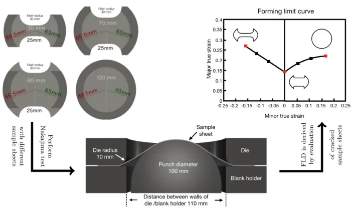
The Nakajima test is a well-known mate- rial test from steel industries to determine the forming limit of sheet metal. It is demonstrated how FE2TI, our highly parallel scalable implementation of the com- putational homogenization method FE

, can be used for the simulation of the Nakajima test. In this test, a sample sheet geometry is clamped between a blank holder and a die. Then, a hemispherical punch is driven into the specimen until material failure occurs. For the simulation of the Nakajima test, our software package FE2TI has been enhanced with a frictionless contact formulation on the macroscopic level using the penalty method. The appropriate choice of suitable boundary conditions as well as the influence of symmetry assump- tions regarding the symmetric test setup are discussed.

In order to be able to solve larger macroscopic prob- lems more efficiently, the balancing domain decomposi- tion by constraints (BDDC) approach has been imple- mented on the macroscopic level as an alternative to a sparse direct solver. To improve the computational effi- ciency of FE2TI even further, additionally, an adaptive load step approach has been implemented and di↵erent

Department for Mathematics and Computer Sci- ence, University of Cologne, Weyertal 86-90, 50931 Cologne, Germany, E-mail: axel.klawonn@uni-koeln.de, martin.lanser@uni-koeln.de, m.uran@uni-koeln.de, url:

https://www.numerik.uni-koeln.de and Center for Data and Simulation Science, University of Cologne, url:https://cds.uni-koeln.de

Oliver Rheinbach

Institut f¨ur Numerische Mathematik und Optimierung, Fakult¨at f¨ur Mathematik und Informatik, Technische Uni- versit¨at Bergakademie Freiberg, Akademiestr. 6, 09596 Freiberg, E-mail: oliver.rheinbach@math.tu-freiberg.de, url:

https://www.mathe.tu-freiberg.de/mno/mitarbeiter/

oliver-rheinbach

extrapolation strategies are compared. Both strategies yield a significant reduction of the overall computing time. Furthermore, a strategy to dynamically increase the penalty parameter is presented which allows to re- solve the contact conditions more accurately without increasing the overall computing time too much. Nu- merically computed forming limit diagrams based on virtual Nakajima tests are presented.

Keywords

Nakajima test

Computational homoge- nization

FE

Finite elements

Frictionless contact

Penalty method

Multiscale

Domain Decomposition

Iterative Solvers

1 Introduction

In this article, we consider the numerical simulation of the Nakajima test on high-performance computers us- ing our highly scalable software package FE2TI [26], which combines an implementation of the computa- tional homogenization approach FE

[17, 38, 44, 53, 55]

with di↵erent domain decomposition approaches such as BDDC (Balancing Domain Decomposition by Con- straints) [10, 13, 40, 42, 43] and FETI-DP (Finite Ele- ment Tearing and Interconnecting - Dual Primal) [15, 16, 34, 35, 36, 37]. It makes use of software packages such as BoomerAMG [21] (see [2] for the scalability of Boomer- AMG for elasticity) from the hypre library [14] and sparse direct solver packages such as PARDISO [51], MUMPS [1], and UMFPACK [11].

The Nakajima test is a material test, well-known in

the steel industry, to determine the forming limits of

sheet metal. A sheet metal is clamped between a blank

holder and a die. Subsequently, a hemispherical punch

is driven into the specimen until a crack occurs; see

Figure 1 (middle). The top surface of the sheet metal is

withdi↵erentsamplesheets PerformNakajimatest ofcracked samplesheets

FLDisderived byevaluation

Fig. 1 Experimental setup of the Nakajima test and derivation of a forming limit diagram (FLD) using the Nakajima test.

Image composed from [59, Fig. 1; Fig. 2.4].

equipped with a grid or a pattern, and the deformation is recorded by cameras. Friction between the sample sheet and the rigid punch has to be avoided as much as possible by introducing a tribological system. For further details regarding the test setup of the Nakajima test, we refer to the ISO Norm [46].

In this article, we consider the simulation of the Nakajima test for a dual-phase (DP) steel. More pre- cisely, we consider a DP600 grade of steel. DP steels be- long to the class of advanced high strength steels and combine strength and ductility. All DP steels have a ferritic-martensitic microstructure consisting of marten- sitic inclusions (hard phase) in a ferritic matrix (soft phase). The favorable macroscopic properties of DP steels are strength and ductility, resulting from the mi- croscopic heterogeneities obtained by a complex heat treatment during the rolling process; see, e.g., [57]. Thus, the incorporation of information on the microstructure into the simulation is necessary to obtain accurate sim- ulation results.

Since the characteristic length scales of the micro- and the macroscale di↵er by 4 to 6 orders of magnitude, a brute force approach using a finite element discretiza- tion down to the microscale, is not feasible, even on the largest supercomputers available today. Moreover, a brute force simulation would require full knowledge

of the microscale for the complete macroscopic struc- ture and would also produce more detailed results than necessary. This motivates the use of homogenization methods. Here, the FE

computational homogeniza- tion method was chosen; see also our earlier publica- tions [32, 26] on the use of FE

within the EXASTEEL project, which was part of the DFG priority program 1648 “Software for Exascale Computing” (SPPEXA, [12]); see Section 2 and the acknowledgements.

In practice, the Nakajima test is used to generate forming limit diagrams (FLDs) and corresponding form- ing limit curves (FLCs); see Figure 1 (top right). An FLD is a Cartesian coordinate system with the major true strains on the

the

pairs of major and minor strains. It describes the tran- sition from admissible to impermissible loads and thus provides information on the extent to which the ma- terial can be deformed without failure, under certain deformation conditions. The di↵erent Nakajima sam- ple geometries (see Figure 1 top left) cover the range from uniaxial to equi-biaxial tension.

Note that material failure is typically indicated by

local necking in thickness direction before a crack oc-

curs. In physical experiments, to reconstruct the state

immediately before material failure, images of the top

surface of the sample sheet are recorded by one or more camera(s). In the algorithmic approach given in the present paper, we instead use a modified Cockroft-Latham criterion to predict material failure; see Section 3. Hence, we do not have to compute the evolvement of a crack.

For a description how the experiment is evaluated to obtain a point in the FLD, we refer to the normed evaluation strategy based on cross sections [46] and to the evaluation strategy based on thinning rates [60]. For the implementation of both strategies and the resulting virtual FLDs and FLCs, we refer to [59, Sec. 2.8, Sec.

2.9, Fig. 3.5-3.7].

In this paper, we will describe the software enhance- ments that were necessary to perform the simulation of the Nakajima test using our FE2TI software pack- age [26]. This includes the implementation of a fric- tionless contact formulation on the macroscopic level using a penalty method, the incorporation of the blank holder and the die into the simulation to approximate the real test setup as good as possible, and the choice of suitable boundary conditions. Furthermore, we high- light the e↵ects of improved initial guesses for each load step using an extrapolation strategy as well as using an adaptive load step strategy. Our further advances, com- pared to [26] and [32] include a parallel Newton-Krylov- BDDC (NK-BDDC) approach (based on [27]) applied to the macroscopic problem, which replaces Newton- Krylov-BoomerAMG used earlier.

The incorporation of NK-BDDC as a parallel solver on the macroscopic level enables us to perform larger simulations without relying on symmetry. Moreover, it allows us, for the first time, to perform simulations con- sidering the full geometries corresponding to the quar- ter geometries that were used for the derivation of the virtual FLDs in [32,59]. As a consequence, we are now able to analyze the e↵ect of mirroring the solution of a quarter geometry to obtain an approximation of the overall solution. We obtain the full geometry that corre- sponds to a specific quarter geometry by vertically and horizontally mirroring the mesh of a quarter geometry;

see Section 5.

Moreover, we show the e↵ect of second-order extrap- olation for computing the initial value of each load step.

We also introduce a strategy to increase the penalty parameter at the end of the macroscopic contact sim- ulation in order to improve the accuracy without in- creasing the computing time too much. Note that while achieving efficiency and parallel scalability to millions of MPI ranks was in the focus of our previous works [26, 32]. Here, we report on production computations us- ing 4 000 to 15 000 cores of the JUWELS supercom- puter [25]. Since limited computing time was available on JUWELS for this project, we have used the fol-

lowing computational setup: All our computations are two-scale finite element simulations where we solve in- dependent microscopic problems for each macroscopic integration point. We consider comparably small micro- scopic problems with 7 191 degrees of freedom resulting from the discretization of the unit cube with P2 finite elements. Each microscopic problem is solved indepen- dently on its own MPI rank and, given its small size, we use the sparse direct solver PARDISO to solve the re- sulting system of equations. We also show results using an identical setup on about 6 000 cores of the magni- tUDE supercomputer. Note that we use two MPI ranks for each compute core. Similar to our previous works (e.g. [32, 26]), we mark macroscopic quantities with an overline to distinguish them from microscopic quanti- ties. For example, we write

for the macroscopic dis- placement and

for the microscopic one.

2 The Software Package FE2TI

For all our simulations presented in this article, we have used our highly scalable software package FE2TI [26].

The core of the FE2TI package is a C/C++ implemen- tation of the computational homogenization approach FE

[17, 38, 44, 53, 55] (see Section 2.1), which enables the incorporation of the microstructure into the simu- lation without the need for a brute force finite element discretization. We extensively use the PETSc library [3, 4, 5] and distributed memory parallelization based on message passing (MPI).

The FE2TI package interfaces di↵erent solvers for the solution of the resulting linear and nonlinear sys- tems of equations on both scales. For small linear sys- tems, the direct solver libraries PARDISO [51] (or MKL- PARDISO), UMFPACK [11], and MUMPS [1] are used.

Here, PARDISO [51] is our preferred sparse direct solver, which we can also use in shared-memory parallel mode [30]; see also [61]. Throughout this paper, each micro- scopic boundary value problem is solved independently on its own compute core.

In order to handle also larger problem sizes effi-

ciently, the software package also gives the possibility

to use a domain decomposition approach or (algebraic)

multigrid for the parallel iterative solution of the result-

ing problem. Larger microscopic boundary value prob-

lems, i.e., representative volume elements (RVEs) with

a large number of degrees of freedom, can be tackled by

using parallel domain decomposition methods based on

Newton-Krylov-FETI-DP (NK-FETI-DP) [27,39,48] or

the more recent Nonlinear-FETI-DP approaches [27,

31]. Here, each RVE is decomposed into subdomains,

where each subdomain is handled by its own compute

core. Accordingly, each microscopic boundary value prob- lem is solved on more than one compute core, depending on the number of subdomains into which the RVE has been split.

As an alternative to domain decomposition, we can also use the highly scalable multigrid implementation BoomerAMG [21] from the hypre package [14] for the parallel solution of the microscopic problem as well as of the macroscopic problems. Here, the extensions of BoomerAMG for elasticity should be used; see [2] for the scalability of BoomerAMG in this case.

Various simulations of tension tests for a DP600 steel have been performed using di↵erent aspects of the software package. In 2015, the FE2TI package scaled to the complete JUQUEEN [24] and became a member of the High-Q club [29]. The combination of NK-FETI-DP on the microscale and BoomerAMG on the macroscale has been considerably successful; see SIAM Review [49, p. 736].

While using BoomerAMG on the macroscopic level works very well for the FE

simulation of di↵erent ten- sion tests [29, 28, 26], its performance su↵ered in our FE

simulation of the Nakajima test, which seems to be challenging for AMG methods. Therefore, we have recently incorporated a second domain decomposition approach, the NK-BDDC method (see, e.g., [27, 39]), in order to solve comparably large macroscopic problems efficiently.

In addition to the NK-BDDC approach, in the sec- ond phase of the EXASTEEL project, we further ex- tended our software package to simulate the Nakajima test. This included frictionless contact (on the macro- scopic level) using a penalty formulation (see Section 2.4), an adaptive load step strategy (see Section 2.2) and first- or second-order extrapolation (see Section 2.3) to improve initial guesses for Newton’s method. We have also integrated a Checkpoint/Restart (CR) strat- egy into our software. Here, we use the CRAFT library [54], which was developed in the second phase of the ESSEX project, also part of SPPEXA [12]. We use two di↵erent checkpoint objects, one for the macroscopic level and one for the microscopic level including the history for each microscopic boundary value problem.

Even for small problem sizes, which can be solved efficiently by using a sparse direct solver, the finite ele- ment assembly process may be computationally expen- sive. Therefore, we have parallelized the assembly pro- cess of the macroscopic problem using a small number of cores, even if we use a sparse direct solver.

Using the FE

two-scale homogenization approach, we only have to provide a constitutive material law on the microscopic level. We use a J

elasto-plasticity model, which is implemented in FEAP [58] and can be

called via an interface provided by our software pack- age. The material parameters are fitted to the main components of a DP steel, namely ferrite and marten- site; see [8].

2.1 The FE

Method

The FE

method [17, 38, 44, 53, 55] requires scale sepa- ration, i.e., the characteristic length

of the macroscale is much larger than the characteristic length

of the mi- croscale, commonly denoted by

is a factor of 10

to 10

larger than the microscopic unit length. Hence, we can assume that scale separation is given.

In the FE

method, both scales are discretized in- dependently of each other by using finite elements. Ac- cordingly, the macroscopic sample sheet geometry is discretized using comparably large finite elements with- out taking the microstructure into account, i.e., we con- sider a homogeneous material from the macroscopic point of view. In each macroscopic integration point (Gauss point), we solve a microscopic boundary value problem. The microscopic boundary value problem is defined on a cuboid with a side length of the order of

all microstructure and is therefore called representa- tive volume element (RVE). Note, that we use the same RVE for each macroscopic Gauss point.

The microstructure of a DP steel can be obtained by using electron backscatter di↵raction (EBSD); see [8].

To reduce the problem size, we make use of the statisti- cally similar RVE (SSRVE) approach, see [7, 52], which can approximate the true mechanical behavior accu- rately. In contrast to the small martensitic islands in a realistic microstructure of a DP steel, the martensitic volume fraction is distributed to only a few and, there- fore, larger inclusions with predefined, simple shapes, e.g., ellipsoids. The number of inclusions is predefined, and the final shape of the inclusions is obtained after an optimization process. In this article, we consider an SSRVE with two ellipsoidal inclusions. We use periodic boundary conditions.

In the FE

method, the macroscopic constitutive

law is replaced by a micro-to-macro coupling procedure

(see, e.g., [53, 18] for the consistent tangent), making

use of volumetric averages of microscopic stresses; see

[53] for further details regarding the FE

approach and

[6, 26] for the incorporation of the FE

method into our

software package.

2.2 Adaptive load step strategy

In our simulations of the Nakajima test, the rigid punch has to cover a significant distance until a critical value

(see Section 3) is reached for at least one finite element node on the top surface of the sample sheet.

To be able to simulate the corresponding distance, we use a load step strategy on the macroscopic level.

We have implemented a simple adaptive load step strategy, which decides, based on microscopic as well as macroscopic events, whether the load increment may be increased (by a factor of 2), decreased (by a factor of 1/2), or if it remains constant.

On the microscopic level, if we reach convergence within 20 Newton iterations, i.e., in a macroscopic New- ton iteration

of load step

of the stresses as well as the consistent tangent moduli are transferred to the macroscopic level. Otherwise, we pass the information that there is stagnation; see Fig- ure 2. In this case, we have to decrease the load step size and repeat the current load step. Note that we refer to stagnation not only if we do not reach convergence within 20 Newton iterations, but also if the residual norm does not decrease sufficiently after the sixth mi- croscopic Newton iteration; see Figure 2. We also use an upper bound of 20 macroscopic Newton iterations per load step. If we do not reach convergence within this range, we decrease the load step size. However, if the residual norm

at the end of the 20th iteration is close to the stopping criterion

tol

the tolerance tol can be chosen by the user, we spend five more Newton iterations in the current load step. If we reach convergence within these five additional iter- ations, we continue with the next load step, otherwise, we have to repeat the current load step.

To decide whether the load increment has to be in- creased or not, we compare the number of Newton iter- ations of the current load step with the corresponding number of the previous load step. If it is at most as large as 50 % of the previous load step, the load incre- ment for the next load step is doubled. Otherwise, the load increment remains unchanged.

We increase the load increment whenever we reach convergence within a single Newton iteration. For a di- agram similar to Figure 2, we refer to [59, Fig. 4.3] and [32, Fig. 6].

To highlight the advantages of our adaptive load step approach, we present a comparison using di↵er- ent constant load step sizes and the adaptive load step strategy choosing the same initial load increments. We consider a sample sheet geometry with a parallel shaft width of 50 mm; see Table 1 for the results; see Figure 1 and Section 4 for the description of the general shape of

the sample sheet geometries. We apply the same three initial load increments for both constant load step sizes and our adaptive load step strategy.

Let us first consider constant loads. For the smallest load increment of 3.125

10

mm, the final computa- tion time is about seven times higher than for a load increment of 0.1 mm. This can be explained by the in- creased number of macroscopic Newton iterations. Even if the load increment is much smaller the time for a sin- gle Newton iteration only decreases slightly. To demon- strate the case of a too large load step, which causes stagnation at some point, we have chosen a load in- crement of 0.2 mm. Here, the simulation terminates within the second load step since at least one micro- scopic boundary value problem does not reach the stop- ping criterion.

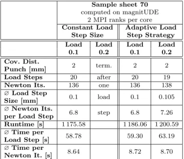
As we learn from Tables 1 and 2, the adaptive load step strategy is, in our context, also robust with re- spect to large initial load step sizes, as, e.g., 0.2 mm.

Additionally, the adaptive load step algorithm delivers small computing times independent of the initial load step. For instance, for the smallest initial load incre- ment, the dynamic load step strategy detects several times that the load step size can be increased. As a result, the average load step size is about ten times larger than the initial load increment. Compared to the constant load, we need only a third of the macroscopic Newton iterations, and we get the same factor also for the computing time.

The fastest computing time is achieved using an ini- tial load increment of 0.2 mm. Even if we have to repeat the second load step with a reduced load increment, the load increment is again increased to 0.2 mm later on.

As a result, the average load step size is close to 0.2 mm. This is di↵erent for a sample sheet geometry with a parallel shaft width of 70 mm. In this case, the load step strategy never increases the load increment back to 0.2. Consequently, the average load increment is close to 0.1 mm and the computing time is slightly higher compared to the case where an initial load step size of 0.1 mm was used, since some load steps are repeated;

see Table 2.

For both sample sheet geometries considered here, the initial load step size of 0.1 mm seems to be optimal, since the adaptive load step strategy does not change the load step size within the first two millimeters. How- ever, if we push the rigid tool further into the sample sheet geometry as it is done to obtain an FLD, the load increment is decreased several times for both geometries by the adaptive load step strategy; see [32, Tab. 3.1];

note that the average load step size can be computed

from the number of load steps.

Macroscopic Newton Iterationiof Load Stepk

Convergence within 20 (mi- croscopic) Newton iterations

No reduction of norm in a microscopic New- ton iteration after the 6th Newton iteration

NoConvergence within 20 (microscopic) Newton iterations

Compute stresses and tan- gent moduli and give them to the macroscopic level

Give information of no convergence to the macroscopic level,reduceload increment load_kby 50%, andrestartload stepk

Continuewith next macroscopic Newton iterationi+ 1 of load stepk

Fig. 2 Impact of microscopic events on the load step size. Image from [59, Fig. 4.2].

Table 1 Comparison of some characteristic quantities for the first 2 mm covered by the rigid punch using di↵erent constant load step sizes as well as the adaptive load step strategy with di↵erent initial load step sizes; computed on the JUWELS supercomputer [25]; using a quarter geometry of the sample sheet with a shaft width of 50 mm; two finite elements in thickness direction. We have used first-order extrapolation and 2 MPI ranks per core. We consider the computation time as well as the number of macroscopic load steps and Newton iterations. Table from [59, Table 4.1]

Sample sheet 50

computed on JUWELS; 2 MPI ranks per core

Constant Load Step Size Adaptive Load Step Strategy

Load Load Load Load Load Load

0.003125 0.1 0.2 0.003125 0.1 0.2

Cov. Dist. 2 2 term. 2 2 2

Punch [mm]

Load Steps 640 20 after 86 20 11

Newton Its. 970 130 one 328 130 91

?Load Step

0.003125 0.1 load 0.0233 0.1 0.18

Size [mm]

?Newton Its. 1.52 6.50 step 3.81 6.50 8.45 per Load Step

Runtime [s] 7 204.58 1 048.61 2 415.89 1 070.00 808.01

?Time per 11.26 52.43 28.09 53.50 73.46

Load Step [s]

?Time per

7.43 8.07 7.37 8.23 8.88

Newton It. [s]

At the onset of material failure, typically small load steps are needed. We indeed use 10 consecutive load steps, using a load increment smaller than 10

multi- plied by the initial load increment, as an indicator for material failure.

Furthermore, we also terminate the simulation if the load increment has to be reduced seven times within a single load step.

2.3 Improved Initial Values by First- and Second-Order Extrapolation

As we have learned from Tables 1 and 2 in the previous

section, the overall computing time strongly depends on

the number of macroscopic Newton iterations. There-

fore, in order to reduce the computing time, we are

interested in reducing the number of macroscopic New-

ton iterations in each load step by using better initial

guesses from extrapolation.

Table 2 Comparison of some characteristic quantities for the first 2 mm covered by the rigid punch using di↵erent con- stant load step sizes as well as the adaptive load step strat- egy with di↵erent initial load step sizes; computed on mag- nitUDE; using a quarter geometry of a sample sheet with a shaft width of 70 mm; two finite elements in thickness di- rection. We have used first-order extrapolation and 2 MPI ranks per core. We consider the computation time as well as the number of macroscopic load steps and Newton iterations.

Table based on [59, Table 4.2]

Sample sheet 70 computed on magnitUDE

2 MPI ranks per core Constant Load Adaptive Load

Step Size Step Strategy Load Load Load Load

0.1 0.2 0.1 0.2

Cov. Dist. 2 term. 2 2

Punch [mm]

Load Steps 20 after 20 19

Newton Its. 136 one 136 138

?Load Step

0.1 load 0.1 0.105

Size [mm]

?Newton Its. 6.8 step 6.8 7.26 per Load Step

Runtime [s] 1 175.58 1 186.06 1 200.59

?Time per 58.78 59.30 63.19

Load Step [s]

?Time per

8.64 8.72 8.70

Newton It. [s]

We are thus interested in predicting the macroscopic displacement at the end of the following load step de- pending on the accumulated load. For simplicity, we assume that we have just finished load step

accumulated loads

=

j=1lj

, where

is the load increment of load step

tions

,

= 1, . . . , k, of the macroscopic displacements in load step

are known. Furthermore, the load incre- ment

has already been determined by the adaptive load step strategy, i.e., the expected accumulated load

lk+1

=

j=1lj

of the next load step is also known.

In case of stagnation in load step

+ 1, the load in- crement

changes, which also causes a change in

. Accordingly, the interpolation polynomial has to be evaluated at a di↵erent point. As a result, the initial value of the repeated load step changes.

To derive an interpolation polynomial of the order

step

+ 1, we need the macroscopic displacements

and the accumulated loads

of the current load step

as well as of the previous load steps

1.

Of course, this is only applicable if

corresponds to an existing load step, i.e.,

1. Note that the accumulated loads of di↵erent load steps di↵er, since each load step makes a small load increment. If we find

a polynomial

of order

(l

) =

(

Xj

m=1

lm

) =

=

(1) then the interpolation polynomial is unique.

In case of a first-order interpolation polynomial, which was already successfully used for the simulation of a tension test with constant load increments (see [26]), we only need the accumulated loads and macroscopic displacements of the load steps

and

1. We obtain the interpolation polynomial

p1

(l) =

+

lk lk

1

(u

)

which satisfies Equation (1). As a result, the predicted solution of load step

+ 1, which is subsequently used as initial value

is derived by

u⁽⁰⁾_k+1

=

(l

) =

+

+

lk ·

(u

)

which di↵ers from the presentation in [26] due to the variable load increments.

All in all this is an extrapolation strategy, since we use the interpolation polynomial to predict the solu- tion of load step

+ 1, where

is not included in the interval

lk 1,lk⇤

. Since

is a polynomial of or- der 1, the use of

for predicting initial values of the following load step is called first-order extrapolation.

This strategy has been successfully applied to compute an FLD (see [32, 59]) and has also been used to compare constant and dynamic load increments in Section 2.2.

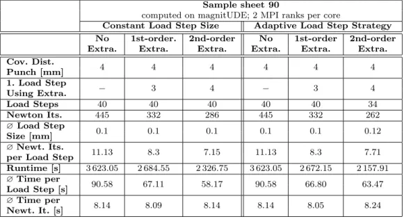
As we learn from Table 3, first-order extrapolation reduces the number of macroscopic Newton iterations significantly, which also causes a reduction in comput- ing times. Let us remark that, for the test setup with an initial load step size of 0.1 mm, the adaptive load step strategy does not change the load step size if used in combination with the first-order extrapolation ap- proach. Therefore, the results for the first-order extrap- olation with and without adaptive load stepping are identical in Table 3. For similar results using a sample sheet geometry with a smaller shaft width and using a quarter geometry, we refer to [59, Tab. 4.3]. We also consider a second-order interpolation polynomial, i.e., we require the accumulated loads and macroscopic dis- placements of the load steps

2, . . . , k. The second- order polynomial

can be formulated in terms of the Lagrange polynomials

Lj

(l) =

m=k 2 m6=j

l lm

lj lm

.

Table 3 Comparison of first- and second-order extrapolation for the first 4 mm covered by the rigid punch with and without using an adaptive load step strategy (see Section 2.2); initial load step size of 0.1 mm; computed on magnitUDE; using a full geometry of a sample sheet with a shaft width of 90 mm; two MPI ranks per core; one finite element in thickness direction.

Table from [59, Table 4.4] .

Sample sheet 90

computed on magnitUDE; 2 MPI ranks per core

Constant Load Step Size Adaptive Load Step Strategy No 1st-order. 2nd-order No 1st-order 2nd-order Extra. Extra. Extra. Extra. Extra. Extra.

Cov. Dist.

4 4 4 4 4 4

Punch [mm]

1. Load Step 3 4 3 4

Using Extra.

Load Steps 40 40 40 40 40 34

Newton Its. 445 332 286 445 332 262

?Load Step

0.1 0.1 0.1 0.1 0.1 0.12

Size [mm]

?Newt. Its. 11.13 8.3 7.15 11.13 8.3 7.71

per Load Step

Runtime [s] 3 623.05 2 684.55 2 326.75 3 623.05 2 672.15 2 157.91

?Time per 90.58 67.11 58.17 90.58 66.80 63.47

Load Step [s]

?Time per

8.14 8.09 8.14 8.14 8.05 8.24

Newt. It. [s]

Finally,

writes

p2

(l) =

i=k 2

ui·Li

(l);

see, e.g., [47]. Obviously, we have

(l

) =

lk lk 2 · lk lk 1

lk lk 1

= 1. (2)

Furthermore, we have

(l

) =

(l

) = 0, since the first or second part in Equation (2) becomes zero if we replace

in the numerators by

or

. In gen- eral, for each three consecutive load steps

+ 2, we have

(l

) =

,

+ 1, m + 2

. Accord- ingly, the second-order polynomial

satisfies Equa- tion (1).

If we now use

to extrapolate the solution of load step

+ 1 to determine an initial value

for load step

+ 1, we obtain

u⁽⁰⁾_k+1

=

(l

) = (l

+

)l

lk 1

(l

+

)

(l

+

+

)l

lk 1lk

uk 1

+ (l

+

+

)(l

+

) (l

+

)l

uk

by replacing

,

=

2, . . . , k + 1, by

j=1lj

and cancelling out all possible terms.

As we learn from Table 3, second-order extrapola- tion is useful in our context since it reduces the num- ber of iterations even more than first-order extrapo- lation – without significant additional computational cost; see [59, Tab. 4.3] for comparable results using a quarter geometry of a sample sheet geometry with a smaller shaft width. Consequently, second-order extrap- olation should be preferred to first-order extrapolation, as long as the available memory allows to store the ad- ditional macroscopic solution values. This might lead to some difficulties considering very large macroscopic problems.

A final remark on the contact constraints: Without applying an extrapolation strategy, the deformation is exclusively driven by the contact constraints. However, if we use the predicted solution of a load step as initial value, the initial value already contains some deforma- tions which are not caused by the contact constraints.

In this case, the contact constraints have to check the predicted deformation and correct it if necessary.

2.4 Frictionless Contact Using a Penalty Formulation In the Nakajima test, the deformation of the sample sheet is completely driven by the hemispherical punch.

Moreover, the deformation is restricted by the blank

holder and the die. Consequently, the simulation of the

Nakajima test requires a contact formulation on the

macroscopic level. As mentioned before, friction between

the rigid punch and the sample sheet has to be avoided

as much as possible in the experiments by using a lu- brication system. Accordingly, in an ideal test setup, which is assumed in our simulations, there will be no friction between the rigid punch and the sample sheet, and we can consider frictionless contact.

We have to incorporate the physical condition of non-penetration into our simulation. Therefore, let us consider an arbitrary rigid tool

and a deformable body

, where only the deformable body

is discretized by finite elements. The contact surface of the rigid tool is represented by an analytical function. We further as- sume that exclusively one face

of the deformable body may be in contact with the rigid tool. For each finite element node

we have to compute the corresponding point

on the rigid tool surface with minimum distance, i.e.,

= min

. Subsequently, we can compute the outward normal

of the rigid tool surface at the minimum distance point

. To ensure that no finite element node on the con- tact surface of the deformable body penetrates into the rigid tool, we can formulate the condition

⇣x

B x_T⌘

·nx_T

0

B 2 _B,

(3)

which is the mathematical formulation of the non-pe- netration condition. For a more detailed discussion re- garding the more general case of contact between two deformable bodies, we refer to [62].

As it is standard practice in finite element simu- lations of continuum mechanical problems, we are in- terested in minimizing an energy functional. Due to the contact problem and the corresponding non-penetration condition (see Equation (3)) we have to consider min- imization with constraints. For this purpose, di↵erent approaches such as the Lagrange multiplier method [41, 45] or the (quadratic) penalty method [41, 45] are known and both approaches are widely used in the context of contact problems; see, e.g., [62]. While the Lagrange multiplier method solves the constrained minimization problem exactly, the penalty method only approximates the exact solution depending on a real positive num-

ber

0, which is called penalty parameter. For

"N ! 1

, the solution of the penalty method is identical

to that of the Lagrange multiplier method, but the re- sulting system of equations becomes ill-conditioned for large penalty parameters. Nonetheless, we choose the penalty method in our simulations, since this approach does not change the number of unknowns in our system and can be easily incorporated into the software. The idea of the penalty method is to solve an unconstrained minimization problem, where the violations of the con- straint(s) are weighted by the penalty term which is added to the objective function of the originally con- strained minimization problem. In the context of con-

tact problems, each finite element node that penetrates the rigid body adds an additional term to the energy functional. Therefore, we have to compute the amount of penetration by

g_N

(x) =

⇢

(x

)

if (x

)

0 0, otherwise;

see Equation (3).

Let us introduce the set

as the collection of all finite element nodes that violate the non-penetration condition, i.e.,

C

=

(x)

0

Then, the penalty term, which is added to the energy functional, writes

Z

C

"N

2

dA.

Due to the additional penalty term in the energy functional, we also obtain additional terms in the right- hand side as well as in the sti↵ness matrix of our re- sulting system, which are obtained by derivation and linearization, respectively. Following [22], the contact part of the sti↵ness matrix can be divided into three parts, where only the main part is independent of the amount of penetration. Since we have small load steps and therefore small penetrations, here, we neglect the remaining two parts in our implementation; see also [59].

Let us further explain the numerical realization of the contact problem using a simple example. We assume that the deformable body in its reference configuration is in perfect contact with a rigid tool. In a first step, the rigid surface moves by a small increment, so that some finite element nodes of the discretized body pen- etrate into the rigid body. Accordingly, we build the corresponding system of equations including the addi- tional contact terms and compute the update of the deformation. Afterwards, we check penetration for the deformed (intermediate) configuration and repeat until convergence is reached.

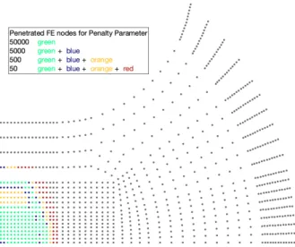
As mentioned before, the choice of the penalty pa- rameter is crucial for the accuracy of the final solu- tion. As you can see in Figure 3, the number of pen- etrated finite element nodes at the end of the simu- lation decreases with an increasing penalty parameter.

Moreover, also the maximum amount of penetration de-

creases as you can see in Table 4. Accordingly, a higher

penalty parameter is desirable to obtain accurate simu-

lation results. On the other hand, we also observe that

a higher penalty parameter leads to significantly larger

computing times; see Table 4; see also [59, Sec. 3.3] for

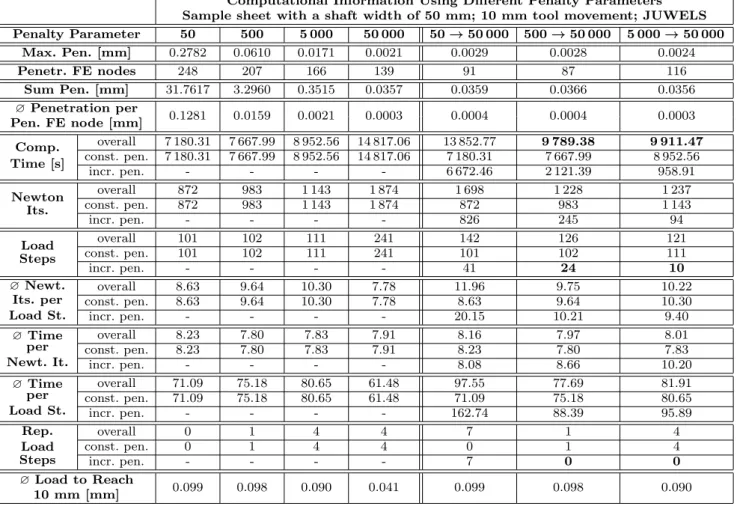
Table 4 Computational results using di↵erent penalty parameters (constant and dynamic) for a sample sheet geometry with a parallel shaft width of 50 mm. If appropriate, e.g., for the computing time, we split the overall collected data into two di↵erent parts of the simulation, namely using a constant penalty parameter (const. pen.) and increasing the penalty parameter to 50 000 (incr. pen.). If we exclusively use constant penalty parameters (first columns), the lines corresponding to the increase of the penalty parameter are left blank and, therefore, the rows “overall” and “const. pen.” are identical. In the columns relating to dynamic penalty parameters, the entries in the rows for constant penalty parameters are identical to the respective entry in the column with the corresponding initial constant penalty parameter; see also Figures 3 and 5. For all simulations with a final penalty parameter of 50 000, we highlight in bold the two fastest overall computation times as well as the main reasons for the fast computation times. Computations carried out on the JUWELS supercomputer [25]; quarter geometry; two finite elements in thickness direction; two MPI ranks per core.

Computational Information Using Di↵erent Penalty Parameters Sample sheet with a shaft width of 50 mm; 10 mm tool movement; JUWELS Penalty Parameter 50 500 5 000 50 000 50!50 000 500!50 000 5 000!50 000

Max. Pen. [mm] 0.2782 0.0610 0.0171 0.0021 0.0029 0.0028 0.0024

Penetr. FE nodes 248 207 166 139 91 87 116

Sum Pen. [mm] 31.7617 3.2960 0.3515 0.0357 0.0359 0.0366 0.0356

?Penetration per 0.1281 0.0159 0.0021 0.0003 0.0004 0.0004 0.0003 Pen. FE node [mm]

Comp.

Time [s]

overall 7 180.31 7 667.99 8 952.56 14 817.06 13 852.77 9 789.38 9 911.47 const. pen. 7 180.31 7 667.99 8 952.56 14 817.06 7 180.31 7 667.99 8 952.56

incr. pen. - - - - 6 672.46 2 121.39 958.91

Newton Its.

overall 872 983 1 143 1 874 1 698 1 228 1 237

const. pen. 872 983 1 143 1 874 872 983 1 143

incr. pen. - - - - 826 245 94

Load Steps

overall 101 102 111 241 142 126 121

const. pen. 101 102 111 241 101 102 111

incr. pen. - - - - 41 24 10

?Newt.

Its. per Load St.

overall 8.63 9.64 10.30 7.78 11.96 9.75 10.22

const. pen. 8.63 9.64 10.30 7.78 8.63 9.64 10.30

incr. pen. - - - - 20.15 10.21 9.40

?Time per Newt. It.

overall 8.23 7.80 7.83 7.91 8.16 7.97 8.01

const. pen. 8.23 7.80 7.83 7.91 8.23 7.80 7.83

incr. pen. - - - - 8.08 8.66 10.20

?Time per Load St.

overall 71.09 75.18 80.65 61.48 97.55 77.69 81.91

const. pen. 71.09 75.18 80.65 61.48 71.09 75.18 80.65

incr. pen. - - - - 162.74 88.39 95.89

Rep.

Load Steps

overall 0 1 4 4 7 1 4

const. pen. 0 1 4 4 0 1 4

incr. pen. - - - - 7 0 0

? Load to Reach

0.099 0.098 0.090 0.041 0.099 0.098 0.090

10 mm [mm]

a similar discussion using a sample sheet geometry with a shaft width of 40 mm.

As a further improvement, we have recently imple- mented a strategy where a small penalty parameter is increased up to a user-defined value if a certain tool movement is reached. Here, significant computing time can be saved in the beginning of the simulation. To dis- tinguish between simulation results obtained with con- stant and increased penalty parameters, we introduce the notation

=

, which indicates that we have increased the penalty parameter to

We show simulation results starting with di↵erent initial penalty parameters and increasing the penalty parameter to

= 50 000 after reaching a total tool movement of 10 mm. As we can see in Table 4, the

overall computing time after reaching the final penalty parameter

= 50 000 is always below the comput- ing time for a constant penalty parameter

= 50 000.

While we save a significant amount of computing time for the initial penalty parameters of 500 and 5 000, the savings for an initial penalty parameter of 50 are neg- ligible. This is related to a large number of additional Newton iterations and repeated load steps to reach the desired penalty parameter

= 50 000 in the end.

We have to ensure that we still obtain an accu-

rate solution. Therefore, we compare the final solutions,

i.e., after reaching the desired penalty parameter

=

50 000, with the solution obtained when using a con-

stant penalty parameter of 50 000. Here, we focus on

the comparison with an initial penalty parameter of

Fig. 3 Penetrated finite element nodes after reaching a total tool movement of 10 mm for the di↵erent penalty parameters

"N = 50 000 (green),"N = 5 000 (green+blue),"N = 500

(green+blue+orange), and"N= 50 (green+blue+orange + red); two finite elements in thickness direction; quarter geometry of a sample sheet geometry with a parallel shaft width of 50 mm (see Figure 1 (top left)); computed on the JUWELS supercomputer [25]. For further information; see Table 4.

500, since we obtain qualitatively similar results for the other penalty parameters; see the apppendix in Sec- tion 7.

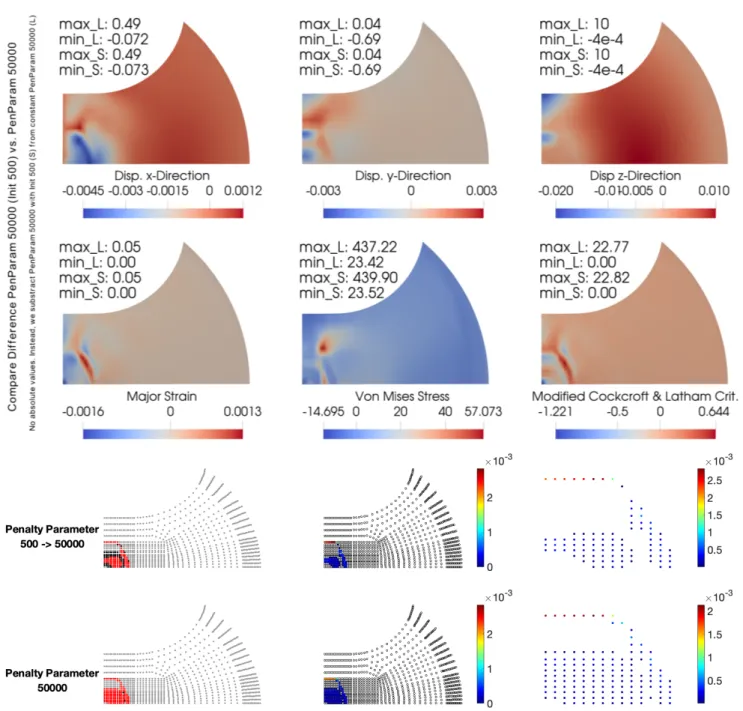
As we can see in Figure 4, the maximum deviation in the displacement is below 1 % in relation to the max- imum absolute value of both solutions. Also for the major strains and the modified Cockcroft & Latham failure value (see Section 3), we obtain a maximum de- viation of about 5 %, which is satisfactory. Only for the von Mises stresses, we obtain a maximum di↵erence of more than 10 %. Surprisingly, the maximum di↵erence in the von Mises stresses is lower if we compare the final solutions obtained with constant penalty param- eters of 500 and 50 000; see Figure 5 (bottom middle).

This might be explained by the penetrated FE nodes.

Comparing the results obtained from constant penalty parameters

= 500 and

= 50 000 with the result obtained after increasing the penalty parameter from 500 to 50 000, the maximum di↵erence is located in the same area, where both solutions have some penetrated FE nodes that are not penetrated in 500

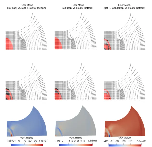
50 000; see Figures 5 and 6. Note that this e↵ect is visible also for other discretizations of the same sample sheet geom- etry; see Figure 7. Nonetheless, our strategy yields convincing results with a significantly reduced overall computing time.

For our simulations of the Najajima test, we increase the penalty parameter based on the failure criterion

since increasing the penalty parameter leads to addi- tional deformations - without movement of the rigid punch. As a consequence, it is possible to reach the critical value while remaining in the same load step.

To guarantee that the critical value is reached for all simulations for the first time with the same penalty pa- rameter, there must be a gap between the critical value that is associated with material failure and the thresh- old used for increasing the penalty parameter.

2.5 Newton-Krylov-BDDC on the Macroscopic Level We have recently incorporated the NK-BDDC approach into our software package in order to solve large macro- scopic problems efficiently.

Of course, good scalability of the overall application can only be achieved if the NK-BDDC approach scales well. Therefore, the choice of a suitable coarse space is essential. A very simple coarse space contains all subdo- main vertices. Due to the thin sample sheet geometry, it is expected that we have too few constraints by choos- ing only the subdomain vertices. Therefore, we choose an additional finite element node along each edge across the subdomain interface in which the primal subassem- bly process is performed. In addition, we also choose constraints for each face across the subdomain inter- face following the suggestions in the frugal approach [20]. For the definition of vertices, edges, and faces in the context of domain decomposition, we refer to the literature; see, e.g., [34, 35, 33].

The incorporation of the NK-BDDC approach al- lows us to use larger macroscopic problems in our sim- ulations. As a consequence, we are now able to consider full geometries corresponding to the quarter geometries used for the derivation of virtual FLDs in [32, 59]. As mentioned before, the mesh of such a full geometry was obtained by vertically and horizontally mirroring the mesh of a quarter geometry and, accordingly, consists of four times as many finite elements.

We find that the number of Krylov iterations in each

macroscopic Newton iteration is in a reasonable range

(see [59, Fig. 3.15 (left)]) and BDDC is robust with re-

spect to the thin geometries and also irregular METIS

decompositions thereof. In our simulations, we always

use GMRES (Generalized Minimal Residual) [19, 50] as

Krylov subspace method. Furthermore, the di↵erence

between minimum and maximum number of Krylov it-

erations is not too large and the average number of

Krylov iterations in each macroscopic Newton iteration

is closer to the minimum. Accordingly, the performance

of the NK-BDDC approach is quite robust and seems

to be independent of the number of macroscopic finite

Fig. 4 Comparison of final simulation results obtained with a constant penalty parameter of 50 000 and after increasing the penalty parameter from 500 to 50 000. Top: Di↵erence in relevant data as well as minimum and maximum values of both configurations; 50 000 (L) and 500! 50 000 (S). Bottom:Comparison of penetrated FE nodes as well as amount of penetration for the final solutions obtained with a constant penalty parameter of 50 000 (bottom) and after increasing the penalty parameter from 500 to 50 000 (top). Red dots show penetrated FE nodes and black dots represent FE nodes that are not penetrated but are penetrated in the other solution; sample sheet geometry with a parallel shaft width of 50 mm; quarter geometry; two finite elements in thickness direction, two MPI ranks per core; computed on the JUWELS supercomputer [25].

elements belonging to the plastic regime, i.e., macro- scopic finite elements with integration points belonging to RVEs in the plastic regime.

3 Failure Detection - a Modified Cockcroft &

Latham Criterion

As mentioned earlier, in the physical Nakajima test, the

hemispherical punch is pressed further upwards until a

crack can be observed on the upper surface of the sam-

ple sheet. Once the Nakajima test is completed, the

Fig. 5 Cross-comparison of penetrated nodes and von Mises stresses for final solutions obtained with constant penalty pa- rameters 500 and 50 000 as well as after increasing the penalty parameter from 500 to 50 000 for a sample sheet geometry with a parallel shaft width of 50 mm; quarter geometry; two finite elements in thickness direction, two MPI ranks per core;

computed on the JUWELS supercomputer [25].

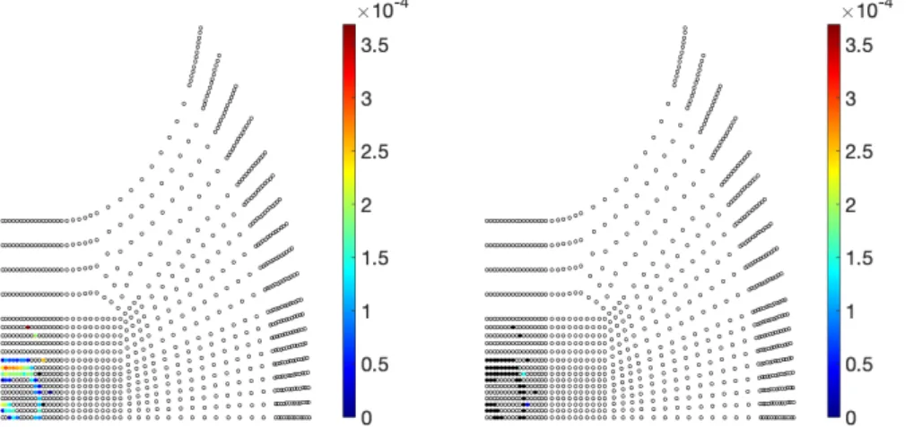
Fig. 6 Penetration of FE nodes that are penetrated in the final solution obtained with a constant penalty parameter of 50 000 but that are not penetrated in the fi- nal solution after increasing the penalty parameter from 500 to 50 000 (left) and vice versa (right);

sample sheet geometry with a shaft width of 50 mm; quarter geoemtry;

two finite elements in thickness di- rection, two MPI ranks per core;

computed on the JUWELS super- computer [25].

sample sheet can be evaluated so that the result can be written into the FLD. In experiments, the evalu- ation process is based on the last recorded image of the sample sheet surface before the crack occurred. In our simulations, we do not end up with a crack since our software does not include the computation of the evolvement of a crack. Instead, we have implemented

a phenomenological failure criterion, where exceeding a prescribed critical value is associated with material failure.

We use a modified version of the Cockcroft & Latham criterion, which was originally presented in 1968; see [9].

In its original version, it depends on the macroscopic

equivalent plastic strain

and the maximum positive

Fig. 7 Cross-comparison of penetrated nodes and von Mises stresses for final solutions obtained with constant penalty pa- rameters 500 and 50 000 as well as after increasing the penalty parameter from 500 to 50 000 with a finer mesh for a sample sheet geometry with a parallel shaft width of 50 mm; quarter geometry; two finite elements in thickness direction, two MPI ranks per core; computed on the JUWELS supercomputer [25].

principal stress

at time

, where the stress depends on the overall macroscopic strain

). It was success- fully used in [56] for a DP800 grade of steel. Note that the maximum principle stress is the maximum eigen- value of the stress tensor, which can be represented by a symmetric 3

3 matrix.

Since we use load stepping, the (pseudo-) time

at the end of load step

computes as accumulation over all time increments up to load step

and, therefore, the evaluation of all quantities at time

is equivalent to the evaluation at the end of load step

✏k

and

instead of

) and

(t

), respectively. With

this notation, the original Cockcroft & Latham criterion

is defined as

fWk

=

("(t

)) =

("

) =

Z "^p_k

0

max (

(✏

), 0) d"

; see [9].

During the simulation, we compute the failure value

in each macroscopic integration point at the end of each load step, i.e., after convergence. Subsequently, we interpolate the failure values from the integration points to the finite element nodes. With numerical in- tegration, we obtain

fWk⇡ Xk

i=1

max (

(✏

), 0)

=

+ max (

(✏

), 0)

("

)

i.e., the failure value

in a single integration point is simply the accumulated sum over all load steps up to load step

as well as

are set to zero and ("

) represents the increment in the macroscopic equivalent plastic strain from load step

1 to load step

When the failure value exceeds a prescribed critical value

in at least one finite element node on the top surface of the sample sheet, we assume that failure oc- curs. Accordingly, the simulation has to continue until this condition is fulfilled and the load step that is as- sociated with material failure strongly depends on the choice of the critical value

.

Using the FE

method, we do not have a consti- tutive material law on the macroscopic level. Conse- quently, we cannot use the macroscopic equivalent plas- tic strain

as suggested in the original Cockcroft &

Latham criterion. Instead, we replace the macroscopic equivalent plastic strain

by the volumetric average

˜

"^p

=

of the microscopic equivalent plastic strain

,

which is denoted as

computes as

Wk

=

(˜

) =

+ max (

(✏

), 0)

(˜

˜

)

As in the originally proposed Cockcroft & Latham cri- terion (see [9]), we prescribe a critical value

. As mentioned before, the choice of the critical value is cru- cial for the time at which failure is detected. Unfortu- nately, to the best of our knowlege, there is no such value provided in the literature for a DP600 grade of steel. Moreover, we do not have experimental data to calibrate

by comparing our simulation results with the experiment. Throughout this article, we have cho- sen a critical value

= 450 MPa. This is motivated by the choice of

= 590 610 MPa in [56], consid- ering the original criterion, for a DP800 grade of steel and the fact that a DP600 steel is less robust compared to a DP800 steel.

4 Sample Sheet Geometries and Appropriate Boundary Conditions

All necessary information regarding the Nakajima test are collected in DIN EN ISO 12004-2:2008 [46], includ- ing the description of the sample sheet geometries as well as the specification of the rigid tools. The recom- mended sample sheet geometries all have a central par- allel shaft and an outer circular shape; see Figure 1 (top left). On both sides of the central parallel shaft, there is a circular section with a given radius, which is called fillet radius; see also Figure 1 (top left). If the circular

section forms a quarter circle without intersecting the outer circular boundary of the sample sheet, there is a connection from the end of the quarter of the circle to the outer circular boundary that is parallel to the shaft;

see Figure 1 (top left).

We consider sample sheet geometries with a length of the parallel shaft of 25 mm and a fillet radius of 30 mm (see Figure 1 (top left)), which both fit to the normed range in [46]. Moreover, the chosen specifica- tions of the rigid tools also fit to the normed range in [46]; see Figure 1 (middle). In addition to the recom- mended sample sheet geometries with a central paral- lel shaft, we also consider a completely circular sample sheet. We choose Dirichlet boundary conditions for all material points on the outer circle.

As mentioned before, the incorporation of the blank holder and the die are necessary to rebuild the real test conditions as good as possible, since these tools are re- sponsible for the final shape of the sample sheet.

By integrating the blank holder and the die into the simulation process, not only the number of contact points increases, but also the number of possible con- tact points grows, since, for example, material points on the top surface of the sample sheet can come into contact with a rigid tool (the die). Accordingly, the de- termination of all contact points takes longer and the problem becomes more complex, since more finite ele- ment nodes add an additional contact term. In order to keep the number of contact points as small as possi- ble, we tested di↵erent strategies to incorporate blank holder and die by prescribing a zero displacement in some material points.

For sample sheet geometries with a comparably small parallel shaft width as well as for the completely circu- lar sample sheet, we fix all finite element nodes between blank holder and die. This is associated with a blank holder force that is high enough that material move- ment between blank holder and die is prohibited. Of course, in this case, it is sufficient to exclusively con- sider the remaining part of the sample sheet and to choose Dirichlet boundary conditions for all finite ele- ment nodes on the outer circle of the remaining part.

This strategy works well for all sample sheet geome-

tries with a parallel shaft width of at least 90 mm as

well as for the completely circular specimen. For sample

sheet geometries with a wider parallel shaft and prohib-

ited material movement between blank holder and die,

the failure zone is located at the fillet radius. This phe-

nomenon is also described in [23] and it is related to the

prohibited material movement between blank holder

and die. As a result, we have to adapt the strategy

for all sample sheets with a shaft width of more than

90 mm. Otherwise, the simulation of the Nakajima test

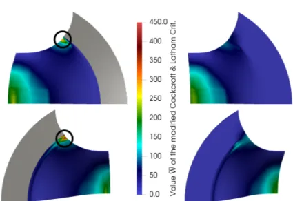
Fig. 8 Comparison of the distribution of the value W of the modified Cockcroft &

Latham criterion (see Section 3) for an overall tool movement of 29.303 mm with prescribed zero displacement for di↵erent material points.

Computation using a quarter geometry of a specimen with a width of 90 mm (see also Fig- ure 1 (left)); two finite elements in thickness di- rection; two MPI ranks per core.Left:Dirichlet boundary conditions completely prohibit ma- terial flow between the blank holder and the die. Part of the specimen between the blank holder and the die is in dark grey; computed on magnitUDE. Right:The usage of adapted boundary conditions enables material flow be- tween the blank holder and the die in the cuto↵

area. Here, we have to simulate the part of the specimen between the blank holder and the die;

computed on the JUWELS supercomputer. Im- age from [59, Fig. 2.5]

would provide invalid results, since the position of the failure zone may not deviate by more than 15 % of the punch diameter from the center of the punch; see [46].

Following [23], material movement is now only pro- hibited for all material points between blank holder and die that have a distance of at most 50 mm to the horizontal center line of the sample sheet. Accordingly, material movement is allowed next to the fillet radius, which results in failure zones along or close to the ver- tical center line; see Figure 8.

Following to the specifications of the rigid tools (see Figure 1 (middle)), for sample sheets with a parallel shaft width of at most 90 mm as well as for the fully circular specimen, we choose Dirichlet boundary con- ditions for all material points

=

p_x, p_y, p_z⇤ q

with

p²_x

+

= 65 mm. For sample sheet geometries with wider parallel shaft widths, all material points with

p²_x

+

= 86.5 mm belong to the Dirichlet boundary and we prescribe a zero displacement for all material points with

p²_x

+

65 mm and

50 mm.

5 Symmetry Assumption

From a macroscopic point of view, under ideal condi- tions, the experimental test setup of the Nakajima test is perfectly symmetric. Accordingly, to save computing time, we have decided to make use of the symmetric test setup, i.e., using the quarter geometry, in most of our simulations including the computation of a virtual FLD (see [32, 59]). Note that our SSRVE, however, does not fulfill the same symmetry conditions; see the discussion below.

For us, exploiting symmetry means to consider only a quarter of the overall sample sheet and to rebuild the

complete solution by mirroring of the solution using the quarter geometry. Continuity of the final solution is guaranteed by additional partial Dirichlet boundary conditions along the boundaries of the quarter geom- etry that belong to the horizontal and vertical cen- ter line of the overall sample sheet. Along the vertical center line, displacement in

(u

= 0). Similarly, the displacement in

set to zero along the horizontal center line (u

= 0). By mirroring the solution obtained for the quarter geome- try, we also mirror the considered microstructure (see Figure 9), which is represented by an SSRVE. In case of an asymmetric structure of the SSRVE, i.e., the posi- tion of the martensitic inclusions change by mirroring, the overall solution violates the condition of a periodic unit cell, since the martensitic inclusions are positioned di↵erently for each quadrant. Consequently, the final solution is only an approximation to the simulation of the complete sample sheet, where the condition of a periodic unit cell is satisfied.

For the derivation of a virtual FLD (see [32, 59]), we have simulated the Nakajima test for several di↵erent sample sheet geometries using quarter geometries. As expected, we have observed that the failure zone evolves along the vertical center line for all sample sheet geome- tries with a parallel shaft width of at least 90 mm. For a parallel shaft width of 100 mm or more, the failure zone does not evolve along the vertical center line but parallel to it. If this happens, rebuilding the solution by mirroring leads to the occurrence of a second fail- ure zone (see [32, Fig. 3.5]). This is not consistent with observations in experiments.

Due to the unexpected position of the failure zone

for sample sheet geometries with a shaft width of at

least 100 mm, we have performed some tests using full

geometries. More precisely, we have used di↵erent meshes