Detection by neuron populations
European Mathematical Psychology Group,
Graz, September 9 – 11, 2008
Uwe Mortensen
University of Münster, Germany
Detection
Probability summation No probability summation
Models of neural mechanisms
The notion of probability summation:
Among channels/mechanisms.
Detection occurs if the activity in at least one of a number of channels exceeds threshold.
Temporal:
Detection occurs if the activity at at least one point of time (within some inerval J = [0, T]) exceeds threshold.
Spatial:
Detection occurs if the activity at at least one point in space (retinal coordinate) exceeds threshold.
Usually just one type of PS is assumed in a given experiment
Probability summation
No probability summation
Aim of detection experiments
Models/
Noise
correlated white
deterministic stochastic
Extreme values theory
Quick‘s model Nonlinear
pooling
Network/popu- lation models
Max mean detection Identification of
neural mechanisms
Inconsistency!
descriptive!
Can be fitted to most data – meaningful?
Theoretical
status unclear!
1
| |
( ) 1 2
n b
i i
c ch
Quick (1974)
Equivalent to Weibull-function
with log 2 absorbed into
( ) 1 c e c b
| | i b i
h
channels spatial positions
| )|
( ) 1 e cht dt
W c
| |
1 p i e ch
ibTemporal PS
Watson (1979) (pooling, Minkowski-
Metric)
Canonical models for PS in visual
psychophysics unit respones
c contrast
Proof/derivation?
Tinkering with maxima of Gaussian variables
Goal directed ad hoc
mathematics
Quotes indicating use of Quick‘s approach:
Similar statements by Meese \& Williams (2000), Tversky, Geisler \& Perry (2004) on contour grouping, Monnier (2006), Meese \& Summers (2007),
… probability summation […] requires that the noises associated with different stimulations be uncorrelated.'' Gorea, Caetta, Sagi (2005, p.2531)
Watson \& Ahumada (2005) take Quick/Minkowski as a basis for a general model of contrast detection – everything is explained (?) Justification: as usual.
''To allow for the statistical nature of the detection process, the effects of
probability summation must be incorporated. … A convenient way to compute the effects of spatial probability summation is based on Quick's (1974)
parameterization of the psychometric function. (Wilson 1978, p. 973; similarly
Wilson, Philips et al 1979, p. 594, Graham 1989, and many others.)
Assumptions:
2 2
0
( 1 exp[ exp[ 1 ( ( ; )) ]]
2 2
) T
c S g t c dt
2 R ''(0)
where the second spectral moment.
2 2
small noise fluctuates slowly large noise fluctuates fast.
Detection and temporal probability summation – correlated noise
0 2
2
1
2 ( ) 1 1 ''(0) ( )
R 2 R o ( ) Noise is Gaussian and stationary
( ) Autocorrelation satisfies
2
2 R ''(0) E [( '( )) ] t 0
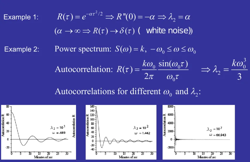
Illustration of second spectral moment:
0 0
Power spectrum: ( ) S k ,
0 0
0
sin( ) Autocorrelation: ( )
2
R k
2 0 3
3 k
0 2
Autocorrelations for different and :
2
/2
( ) ''(0) 2
R e R
( R ( ) ( ) ( white noise) )
Example 1:
Example 2:
Roufs & Blommaert (1981): Determination of the impulse and step response by means of the perturbation technique
Data: Prediction
( , ) e
.079, 1/12.67, 3
p t
g t c c t
b p
Temporal probability summation or maximum mean detection?
2For all values
of !
Stimulus
Pre-filter (lens, retina, LGB) Hebb‘s rule
implies adaptation of neuron – local matched filter
Detection by a population of matched neurons
Defined by a
DOG-function
Test of matched neuron model: no probability summation of any sort!
Stimulus Response of pre-filter
Response of
matched neurons Data and predictions
To be estimated: four free parameters of the pre-filter!
„Channels“ and neuron populations: a stochastic model
Channel = Population of N neurons
( , ) [ , ]
n t t a t number of active neurons within t t t . ( , )
n t t a t N
proportion of active neurons
0
( , )
( ) lim 1 a
t
n t t t
A t t
t N
activity of population at time
The meaning of activity
(based on a model of Gerstner (2000))
( ) 1
( ) ( ) ( )
i
N f ext
i ij j
j
I i
I t w t t I t
Input current for the -th neuron
w ij synaptic coupling of -th neuron with i j th neuron ,
( )
( )
( j f
f j
t t
t
) time course of postsynaptic current generated by spike at time
ext ( )
I t is mean response of sensoric neurons activating observed population
0 /
w ij k N homogeneous case: all-to-all coupling
0 0 excitatory k
0 0 inhibitory k
0 0 independence
k
( ), 1,...,
i
m i i
du u RI t i N
dt Integrate-and-fire neurons:
m RC
time constant of cell membrane
r i
u u
Activity of an individual neuron
Threshold (spike generation) Resting potential
Membrane potential of
i-th neuron
0
0
0 0
( , )
( , ) ,
u u
N u
n u u u
p u t du N
lim
Membrane potential density
0 0
( , )
n u u u N
0 0
u u u
Proportion neurons with membrane potential between and
Membrane potential density
( , ) ( , )
p u t p u t
Taylor-expansion of Fokker-Planck-equation for
Stochastic differential equation for individual trajectory of u:
( , )
specify activity specify p u t
2
0 0
( ) [ ( ) ( ) ( )] ( ) ( ),
( )
ext
r
du t a u t I t t dt t dW t
u u t
Activity.from stimulus
Activity from environment
Derivative of
Brownian motion = white noise
( ) is restricted to this interval!
u t
Drift Diffusion
0 0 0
( ) [ ( ) ext ( ) ( ))] ( ) ( ),
du t a u t I t t dt k t dW t
( ) ( )
varies slowly compared to stimulus driven activity ( Leopold, Murayama,Logothetis, 2003)
determines i the level of activation not due to stimulus, and ii its variance,
constant within trial, varies randomly between trials.
2
0 0
( ) [ ( ) ( ) ( )] ( ) ( ),
( )
ext
r
du t a u t I t t dt t dW t
u u t
Response to short pulses and step functions
( ) ( ) exp( )
I ext t c at p at ( Roufs & Blommaert, 1981)
15.5 7.5 2.5
1. The amplitude of mean response g is the same in all three cases – the smaller eta, the more pronounced is g
2. The peaks of the activity (spike rate) are extremely short compared to the mean response to the stimulus – prob. summation is unlikely!
(Response to a 2 ms pulse!)
g x 0
S
max
Detection model:
Ground activity: determines probability of false alarm Maximum of mean activity
Noise (= activity) from environment ( > 0)
Threshold value
Yeshurun & Carrasco, 1998, 1999; Treue, 2003; Martinez-Trujillo &
Treue, 2004: focussing attention on a position or feature will reduce noise and enhance the response.
However: Reynolds & Desimone, 2003: attention increases contrast gain in V4-neurons…
The probability of detection depends on how pronounced the (mean) activity generated by the stimulus is with respect to the overall activity.
Operationalised:
Summary:
1. Quick‘s (1974) model (white noise) may lead to arbitrary interpretations of data
2. Correlated activity is the norm, not the exception
3. More realistic models (correlated noise) of probability summation show that probability summation is not a general mode of detection with max-mean or peak detection a special case
4. There may be adaptive processes – mechanisms are not necessarily invariant with respect to stimulation
5. Construct dynamic network or population models, - not diffuse
„nonlinear summation“ models
Thank you for your attention!
0
( ) 1 exp[ 1 exp[ ( ( , ))] ]
Gauss: c T S g t c dt
T
0
( ) 1 exp[ 1 ( ( , ) ) ], 0
Weibull: c T g t c S dt with S
T
Probability summation over time - the white noise case:
Application of extreme value statistics for independent variables
0
(0) 1 exp[ 1 ( ) ] 1 exp[ ( ) ], 0
T
S dt S S
T
0
(0) 1 exp[ 1 exp( ) ] 1 exp[ ( )]
T
S dt exp S
T
(0) 0 independent of T
1 exp[ ( ) ] (0) 1 exp[ ] , 0
T
t dt T
But:
Detection by TPS, Gaussian coloured noise
The form of the psychometric function and its approximation by a Weibull function; different stimulus durations .
Mean response g(t) Psychometric function:
2 2
0
( 1 exp[ exp[ 1 ( ( ; )) ]]
2 2
)
Tc S g t c dt
Does not approach the
expression for white noise if
lambda-2 approaches infinity!
Roufs & Blommaert (1981): Direct measurement of impulse and step responses by means of a perturbation technique.
Impulse response, transient channel, as determined by perturbation method
Impulse response, as derived from
MTF: true according to Watson (1981)
(although the additional assumption of
Roufs & Blommaert (1981): Direct measurement of impulse and step
responses by means of a perturbation technique (assuming maximum-of-mean detection).
Impulse response for transient channels: 3- or 2-phasic?
Watson (1981):
triphasic impulse response is an artifact
Quick‘s model with exponent between 2 and 7 yields 3-phasic impulse repsonse. True response is 2-phasic, as derived from MTF.
Artifact?
Assumption of
peak
detection?
probability
summation?
Templates or matched filters for circular discs of different diameters,
superimposed on subthreshold Bessel-Jo-patterns for various spatial frequency parameters: neither temporal nor spatial probability summation.
Spatial probability summation:
Data and predictions of template/MF-model, based on temporal peak detection
There is no „nonlinear Minkowski-summation claimed by Watson &
Ahumada (2005) as a necessary element in the detection process!
Determination of line spread function – Hines (1976)
Rentschler & Hilz (1976) – Disinhibition in LSF-measurements?
Disinhibition?
Flanking line about 75% of test line!
Wilson, Philips et al (1979) – no disinhibition, but spatial
probability summation, as modelled by Quick‘s rule
LSF and LSF-estimates – probability summation, correlated noise
p(false alarm) = .1
LSF and LSF-estimates – probability summation, correlated noise
p(false alarm) = .01
Probability summation: correlated noise
(q: luminance proportion of flanking lines, P(fA) = .1 )
Probability summation does not predict disinhibition, - rather, inhibition!
No pseudo-disinhibition for „white noise“!
Pseudo-inhibition for higher flanking
contrasts, no pseudo-disinhibition!
LSF-prediction by Quick‘s rule; stimulus configuration A
Explore mechanisms
Prob. Summation. No Prob. Summation
Correlated noise
White noise
Deterministic
models Stochastic
models
Quick (1974)
1
| |
( ) 1 2
n b
i i