Detection of aperiodic test patterns by pattern specific detectors revealed by subthreshold summation

Abstract. The hypothesis that the visual system de- tects, under certain conditions, stimulus patterns by means of ®lters matched to these patterns (Hauske et al. 1976) may be challenged by the argument that other coding mechanisms like spatial frequency channels, Gabor or Hermite ®lters mimick the behaviour of matched ®lters, a view supported by the ®nding of non- linear contrast-interrelationship functions (CIFs), as determined in superposition experiments. In this paper we argue that an overall non-linear CIF does not contradict the hypothesis of detection by a single matched ®lter: we ®nd that the sensitivity functions determined in our experiments can be separated into two components re¯ecting (i) a bandpass ®lter and (ii) a ®lter characterised by the spectrum of the test- pattern.

1 Introduction

The visual system may be conceived as a neural network composed of subunits acting as ``channels'. Hauske, Wolf and Lupp (1976) proposed the hypothesis that channels matched to certain stimulus patterns exist and were the ®rst to provide threshold measurements, arrived at by an adaptation of the superposition method of Kulikowski and King-Smith (1973), supporting the hypothesis; Hauske, Lupp and Wolf (1978) elaborated the hypothesis and presented more data.

The model of Hauske et al. (1976) has been criticised as being implausible as a general model of pattern detection since it is uneconomical to have special de- tectors for each possible pattern; pattern detection mechanisms should be multipurpose systems respond- ing to a variety of patterns. Graham (1989) claimed that data supporting the model could alternatively be

explained particularly in terms of models of detection by probability summation, e.g. probability summation among spatial frequency channels (Sachs et al. 1971;

Graham 1977, 1980; Watson 1982), or probability summation among channels de®ned by DOG functions, like Wilson and Bergen (1979). Models that may be considered hybrid models of feature detection and de- tection by probability summation, e.g. Daugman (1984); Jaschinski-Kruza and Cavonius (1984); Ross et al. (1989); Du Buf (1992, 1994) may also be taken as competing with the matched ®lter model; however, quantitative tests of the claim that models like these are indeed equivalent to the matched ®lter model do not seem to exist.

However, the matched ®lter model becomes interest- ing again if one takes processes of perceptual learning into account (Beard et al. 1995; Poggio et al. 1992;

Kirkwood et al. 1996); indeed, it is possible to show that Hebb's rule (Hebb 1949; cf. Hertz et al. 1991) together with the suplementary condition that synaptic weights should not become in®nite implies that a neuron will turn into a matched ®lter for a certain stimulus aspect with probability 1 (Oja 1982; Nachtigall 1991). This does not yet mean that the human visual system actually behaves this way, but it appears to be worthwhile to explore to what extent data may be found that support the matched ®lter model.

The purpose of this paper is to present further data concerning the matched ®lter hypothesis and to discuss some conditions which ± it seems ± have to be satis®ed if the superposition method is to reveal detection by matched ®lters. Additionally, we note some properties of parameter estimates that may blur the image of the channels involved in the detection task as generated by the superposition method. In summary, we may say that our experimental results suggest that for the matched

®lter model to ®t the data, the stimulus patterns have to be small and the experimental situation has to be such that cognitive processes like attentional focussing, usu- ally not taken into account by models of elementary detection processes, generate no additional variance in the data.

Correspondence to: U. Mortensen

Detection of aperiodic test patterns by pattern speci®c detectors revealed by subthreshold summation

G. Meinhardt, U. Mortensen

Westf. Wilhelms-UniversitaÈt, MuÈnster, Germany

Received: 16 December 1996 / Accepted in revised form: 9 June 1998

2 Theory

2.1 Notation, de®nitions and assumptions 2.1.1 Notation

Stimulus patterns will be de®ned as s ˆ m

t

s

t

‡ m

b

s

b

, where s, s

t

and s

b

de®ne luminance as functions of the retinal coordinate x; we restrict ourselves to one- dimensional patterns. s

t

will be called the test pattern, s

b

the background pattern. m

t

and m

b

are Maxwell contrasts, de®ned by m ˆ …l

max

ÿ l

min

†=2l

0

, with l

max

and l

min

the maximum and minimum luminance, respectively, and l

0

the average luminance.

A channel is some subsystem of the visual system; we restrict ourselves to linear channels. Let r be the re- sponse of a channel C to the input s. We write r ˆ L…s†, L an operator representing the channel C. Then r ˆ m

t

L…s

t

† ‡ m

b

L…s

b

†; h

t

:ˆ L…s

t

† and h

b

:ˆ L…s

b

† will be called the unit responses of the channel C to s

t

and s

b

, respectively, because they are the responses of C to s

t

and s

b

with contrast equal to 1. r, h

t

and h

b

are functions of x.

2.1.2 Matched ®lters and matched channels

We make use of the standard de®nition of a matched

®lter: let u be a signal with Fourier transform U , and let the signal be processed by a linear system with system function V . The system is matched to the signal u, if V …x† ˆ aU

…x† exp…ÿjxx

^‡

†, where U

is the complex conjugate of U, x ˆ 2pf , f ÿ in our case ÿ a spatial frequency, and x

^‡

the position of maximum output of the system; a is some proportionality constant and j ˆ 

p ÿ1

(cf. Papoulis 1981).

In order to apply the notion of a matched ®lter to the visual system, one has to consider the possibility that the site of the ®lter is cortical, i.e. the ®lter responds to a signal that results from the stimulus pattern s being passed through the retina, the lateral geniculate nucleus, etc. These stages will be called a pre-®lter; the pre-®lter may be represented by a system function G…x†. Let u

t

be the response of the pre-®lter to the stimulus pattern s

t

, and let the Fourier transform of s

t

and u

t

be given by S

t

and U

t

, respectively. Then U

t

…x† ˆ G…x†S

t

…x†. Let us assume that u

t

is detected by a ®lter matched to u

t

. The system function of this ®lter is then V

t

…x† ˆ a

t

U

_t

…x†e

^ÿjxx‡

ˆ a

t

…G…x†S

t

…x††

e

^ÿjxx‡

(see Fig. 1). The ®lter will be referred to as a matched channel for s

t

.

Let us consider the matched channel for s

t

…x† ˆ s

0t

…x ÿ x

0

†, i.e. for a pattern di€ering from a given, foveally presented pattern s

0t

only by a shift with respect to the x-axis. From measurements of the line spread function (LSF) of the visual system, it is known

that the shape of the LSF depends upon the retinal lo- cation (e.g. Hines 1976; Wilson and Giese 1977). Cor- respondingly, we assume that the pre-®lter described by G depends upon x

0

, and so we write G…x; x

0

†. Note that we allow for the special case G…x; x

0

† G

0

, G

0

a con- stant independent of x, perhaps even of x

0

, i.e. we allow for the possibility that there is no separation into a pre-

®lter and a cortical ®lter. The matched ®lter for the shifted pattern s

t

…x† ˆ s

0t

…x ÿ x

0

† with Fourier transform S

t

is de®ned by U

_t

…x; x

0

† ˆ a

t

G

…x; x

0

†S

_t

…x†e

^ÿjxx‡0

, where x

^‡₀

is the locus of maximum output of this ®lter.

Since S

t

…x† ˆ S

0t

…x†e

^ÿjxx0

, the system function of the matched channel is then given by

W

t

…x; x

0

† ˆ a

t

jG…x; x

0

†j

²

S

_0t

…x†e

^{jx…x0ÿx‡0†}

…1†

Note that a

t

is a free parameter in (1) related to the energy of the signal (Papoulis 1981, chapter 6). Figure 1 shows the corresponding cascade.

2.1.3 Contrast interrelation

Suppose that a pattern s ˆ m

t

s

t

‡ m

b

s

b

, i.e. a superpo- sition of the patterns m

t

s

t

and m

b

s

b

, is presented with the contrasts m

t

and m

b

assuming values such that the probability of detection of s equals a certain constant p

0

, e.g. p

0

ˆ 1=2 or p

0

ˆ 3=4. We may write m

t

ˆ /…m

b

†, expressing the fact that for a ®xed value of p

0

, the contrast m

t

has to assume a certain value depending upon that of m

b

once m

b

has been ®xed. / will be called a contrast-interrelationship function (CIF). The indices t and b may be dropped if there is no possibility of confusion: we may put m ˆ m

b

, /…m† ˆ m

t

.

While for s

t

an arbitrary ± e.g. a bar or a sawtooth ± pattern will be chosen, s

b

will de®ne a sinusoidal grating.

It will be shown (Sects. 2.2 and 2.3) that under certain conditions the unit response h

b

to s

b

of a matched channel C

t

for s

t

± provided such a channel exists ± turns out to be proportional to the system function of C

t

, and h

b

is found via the experimental determination of CIFs for the composite pattern s ˆ /…m†s

t

‡ ms

b

.

2.1.4 Dominance

Suppose there exists a set D ˆ fC

1

; . . . ; C

n

g of channels which may become involved in the detection task. Let F

k

ˆ 1 ÿ P

k

with P

k

being the probability that the channel C

k

2 D detects the pattern /…m†s

t

‡ ms

b

. Sup- pose there exists a channel C

l

2 D and a corresponding interval of contrast values M

l

ˆ fmj0 < m < m

l‡

g for some m

l‡

> 0 such that for all m 2 M

l

, F

l

< 1 and F

k

ˆ 1 for k 6ˆ l. Then the channel C

l

is said to dominate the detection process on M

l

.

The idea behind the notion of dominance is that for a certain range, i.e. interval M

l

, of values of m, the e€ects

Fig. 1. The structure of a matched

channel, the notation is given in

the Fourier domain

of probability summation or non-linear pooling of channel activities do not exist or are at least negligible:

for all m 2 M

l

, detection is by a certain single channel C

l

; C

l

will be called the dominating channel

¹

for s ˆ m

t

s

t

‡ m

b

s

b

.

2.1.5 Assumptions

We make the following assumptions:

A

1

(Matched ®lter) For stimulus patterns s

t

as de®ned in sect. 3.1.2 (with s

0t

representing the special case x

0

ˆ 0), detection will be dominated by a single channel C

l

ˆ C

t

, and C

t

has the system function (1), i.e. C

t

is a channel matched to s

t

.

A

2

(Detection) The pattern will be detected with prob- ability p

0

if

r

t

ˆ /…m†h

t

‡ mh

b

ˆ c …2†

c a certain constant, with r

t

ˆ r

t

…x

^‡₀

†, h

t

ˆ h

t

…x

^‡₀

† and h

b

ˆ h

b

…x

^‡₀

†, and x

^‡₀

is the retinal coordinate at which the output of C

t

is maximal.

Comments. A channel may be matched to a pattern without being dominant. However, our method of testing the hypothesis of detection by a matched channel presupposes that the channel is dominant in order to show up as a matched channel (see Sect. 2.3.1); while it is hard to assign a value to m

l‡

in advance, it should be understood that m

l‡

should be suciently large to allow for di€erent values of m < m

l‡

for which di€erent values /…m† ^ can be reliably estimated provided s

t

and s

b

are such that /…m† 6ˆ constant.

It is also implied that the matched channel is location- speci®c, i.e. is speci®c for the retinal position at which the pattern is presented. Hauske et al. (1976) appear to be the ®rst who discussed detection of patterns with respect to (1). It should also be noted that the existence of a matched channel for an arbitrary pattern is not postulated; we only consider detection of patterns by a matched ®lter for each of the patterns employed in the

experiment. (

2.2 Grating sensitivity of a channel matched to s

t

Let s

b

be a sinusoidal grating, i.e. let either s

b

ˆ sin…xx†

or s

b

ˆ cos…xx†, with x ˆ 2pf and f the spatial frequency. Given appropriate conditions (m ˆ m

b

has to be suciently small; if m is too large, the pattern s may be detected by a channel maximally sensitive to s

b

and h

b

is no longer the unit response of the channel C

t

), the unit response h

b

of C

t

is the (harmonic) steady-state response of C

t

. Clearly, h

b

depends upon the value of x.

Since for an arbitrary linear system with system response

W one has L…e

^jxx

† ˆ W …x†e

^jxx

(e.g. Hsu 1970, p. 124) one ®nds, making use of Euler's relations,

h

b

…x; x† ˆ h

^cos_b

…x; x† :ˆ L…cos…xx†† ˆ Re…W …x†e

^jxx

† h

^sin_b

…x; x† :ˆ L…sin…xx†† ˆ Im…W …x†e

^jxx

† 8 <

:

Substituting for W the expression for W

t

given in (1), one has for x ˆ x

^‡₀

, i.e. for the point of maximum output,

h

b

…x

^‡₀

; x†ˆ a

t

jG…x; x

0

†j

²

Re‰S

_0t

…x†e

^jxx0

Š; s

b

…x†ˆ cos…xx†;

a

t

jG…x; x

0

†j

²

Im‰S

_0t

…x†e

^jxx0

Š; s

b

…x†ˆ sin…xx†;

8 <

:

…3†

with S

0t

the Fourier transform of s

0t

and S

_0t

its complex conjugate. Note that according to (1) the system function depends upon x

^‡₀

; taking, as in (3), the response at x

^‡₀

implies that x

^‡₀

no longer shows up on the right hand side of (3), which again means that no speci®c assumptions about the value of x

^‡₀

have to be made. We will therefore simply write h

b

…x† when it is necessary to indicate the dependency of h

b

upon x. Thus the unit response h

b

…x† equals the system function of C

t

. h

b

…x†

will also be referred to as the grating sensitivity of C

t

.

2.3 Estimation of channel characteristics 2.3.1 Estimation of the grating sensitivity

Assumption A

2

implies /…m† ˆ c=h

t

ÿ mh

b

=h

t

for m 2 M

l

ˆ M

t

(since C

l

ˆ C

t

), i.e. the linearity of the CIF on M

t

. The parameters a

t

:ˆ ÿh

b

=h

t

, b

t

:ˆ c=h

t

may be estimated from the pairs …m; /…m††, where ^ / ^ is the experimentally determined estimate of / corresponding to m. Further, b

_t

ˆ /…0† ˆ m

0t

, m

0t

the threshold contrast for s

t

when presented without the background pattern s

b

, and m

0t

h

t

ˆ c. It follows that a

t

=b

t

ˆ ÿh

b

=c.

On the other hand, /…m† ˆ b

_t

‡ a

t

m implies a

t

ˆ …/…m† ÿ b

_t

†=m and a

t

=b

_t

ˆ …/…m† ÿ b

_t

†=…m

0t

m† ˆ ÿh

b

=c. Let ^ a

t

and ^ b

_t

be estimates of a

t

and b

_t

, and let

` ˆ' stand for `is an estimate of'. We introduce the b sensitivity estimates U

i

, i ˆ 1; 2:

U

1

…x; x

0

† ˆ def ÿ ^ a

t

…x†

b ^

_t

ˆ b h

b

…x; x

0

†

c …4†

U

2

…x; x

0

† ˆ def ÿ /…m; ^ x† ÿ m ^

0t

^

m

0t

m ˆ b h

b

…x; x

0

†

c …5†

We have written ^ a

t

…x† instead of ^ a

t

in order to stress the fact that the slope a

t

of the CIF depends upon x, since h

b

depends upon x. ^ b

_t

should be independent of x.

Comments.

1. The calculation of U

1

requires the estimation of the slope a

t

and the additive constant b

_t

of the linear approximation to a CIF, i.e. is based upon the de- termination of a part of a CIF. Therefore, U

1

sum- marises, for a given x, threshold estimates / ^ for di€erent values of m. U

2

, on the other hand, allows

1

The de®nition of dominance may be relaxed somewhat, de-

manding only F

l

< F

k

ˆ 1 ÿ

k

< 1, where the

k

are suciently

small numbers such that the slope of the linear approximation /

_l

approximates ÿh

lb

=h

lt

to a fair degree. However, such an ap-

proach would require a lengthy discussion of the resulting ap-

proximations, which is beyond the scope of this paper. We return

to the question of dominance in the Discussion.

us to arrive at an estimate of ÿh

b

…x†=c on the basis of a single threshold determination /…m† ^ for a given value of m (and x), provided the estimate m ^

0t

is available. One has to assume, of course, that the value of m is from an interval M

t

upon which the CIF is linear. The advantage of using U

1

is that the estimates of ÿh

b

=c are more stable, being based on more measurements, and that the observed section of the CIF allows an appreciation of the requirement of linearity of this section which is necessary to allow the interpretation of U

1

being an estimate of ÿh

b

=c.

The clear advantage of using U

2

is speed of experi- mentation.

The equations (4) and (5) or equivalent versions of them may of course also be found in the work of Kulikowski and King-Smith (1973)

²

and Hauske et al. (1976).

2. If ^ a

t

and ^ b

_t

are determined as Least Squares esti- mates, they will be unbiased (Kendall and Stuart 1973, p 81); however, the quotient even of unbiased estimates need not be unbiased (Kendall and Stuart 1969, p 227).

³

A bias may, in particular, create the impression of a mis®t of model and data even if the model is correct. The bias may, however, be negli- gible if the variances of the estimates ^ a

t

and b ^

_t

(or, equivalently, / ^ and m ^

0t

) are suciently small.

3. Like a

t

, c is a free parameter in our model. Without further assumptions, neither a

t

nor c can be esti- mated from the data; we will concentrate on the fact that according to (1) the system function W

t

of a matched ®lter is proportional to the complex con- jugate of the spectrum of the signal to which the

®lter is matched. We will comment upon the esti- mation of a

t

in the Discussion.

4. If dominance of the detecting ®lter is lacking, a change of m to m

⁰

may imply that the detecting channel changes from C

t

to C

_t⁰

, or the mixture of detecting channels changes to another mixture. This will be the case when channels with similar responses to the stimulus pattern compete with each other under threshold conditions to the extent that in di€erent trials the stimulus may be detected by dif- ferent channels. Since there is practically no physi- cal, in particular no physiological, system which is free of noise (Gardiner 1990), lack of dominance will most likely be due to detection by probability sum- mation for all values of m, which again implies that for no value of m does the CIF re¯ect the charac-

teristics of a single channel. (

Unfortunately, we do not know in advance whether a dominant channel exists for the stimulus patterns employed. Even if we knew, we still might not know the interval M

t

. However, if the sensitivities U

i

do re¯ect the spectrum of s

t

according to (3) we may take this as support of the hypothesis of detection by a dominant, matched channel. If they do not, the detecting channel is either not matched, or not dominant, or neither matched nor dominant. A possible hint for the lack of dominance is that (i) the estimates b ^

_t

for di€erent values of f ˆ x=2p show systematic deviations from m ^

0t

, i.e.

depend upon f , and/or (ii) that the estimates U

1

and U

2

deviate from each other by more than experimental error.

2.3.2 Estimation of the pre-®lter

The factor a

t

jG…x; x

0

†j

²

=c has to be estimated from the data in order to evaluate the matched-channel model. If U

i

…x†, i ˆ 1; 2, is divided by either the real or the imaginary part of S

0t

e

^jxx0

, which again is known from the de®nition of the stimulus patterns, one obtains, according to (3), an estimate of B…x; x

0

† ˆ

^def

a

t

jG…x; x

0

†j

²

=c, depending upon the phase (sine or cosine) of the background grating. Experimental error would imply di€erent estimates for each phase of s

b

. However, these estimates may be summarised into a single estimate B…x; ^ x

0

† of a

t

jG…x; x

0

†j

²

=c, namely B…x; ^ x

0

† ˆ a

t

jSj



…U

^cos_i

†

²

‡ …U

^sin_i

†

²

q

b

ˆ a

t

c jG…x; x

0

†j

²

…6†

jSj is the modulus of S

_0t

e

^xx0

. Equation (6) follows directly from the de®nition of U

i

, i ˆ 1; 2.

One may then predict the observed sensitivities U

i

…x; x

0

† according to

B…x; ^ x

0

†Re‰S

_0t

…x†e

^jxx0

Š ˆ b U

^cos_i

…x; x

0

†Š; s

b

ˆ cos…xx†

B…x; ^ x

0

†Im‰S

_0t

…x†e

^jxx0

Š ˆ b U

^sin_i

…x; x

0

†Š; s

b

ˆ sin…xx†

…7†

i.e. one has to multiply the estimate B…x; ^ x

0

† with either the real or the imaginary part of the spectrum of the stimulus pattern s

t

in order to arrive at a prediction of the measured sensitivities U

^cos_i

…x; x

0

† or U

^sin_i

…x; x

0

†. For given s

t

, spatial frequency f ˆ x=2p and contrast m the value of U

i

…x; x

0

† was determined several times, so that the standard deviation of the lefthand side of (7) can be computed and indicated by error bars. The curve computed according to the lefthand side of (7) can then be directly compared with the values of U

i

…x; x

0

† ˆ U

^cos_i

…x; x

0

†, or U

i

…x; x

0

† ˆ U

^sin_i

…x; x

0

†, de- pending upon the phase of s.

⁴

Note that the factor a

t

=c does not have to be esti- mated when predictions for a given stimulus pattern are

2

Kulikowski and King-smith (1973) introduced the contrast m

0

, usually not from the interval C

t

, such that /

_t

…m

0

† ˆ b

_t

‡ a

t

m

0

ˆ 0.

Then 1=m

0

ˆ ÿa

t

=b

_t

ˆ ÿh

b

…x†=c according to (4); m

0

is the con- trast of s

b

…x† necessary to lift the activation of C

t

to threshold value if activated by a sinusoidal grating of frequency f ˆ x=2p. Since the reciprocal of a threshold contrast is often called `sensitivity' we have thus a further motivation for calling h

b

(or h

b

=c for our purposes) the spatial frequency sensitivity of C

t

. Of course, m

0

is an extrapolated value.

3

This follows from the fact that the expected value of a quotient does, in general, not equal the quotient of the corresponding expected values.

4

Alternatively, one could have ``predicted'' Re‰S

_0t

…x†e

^jxx0

Š and Im‰S

_0t

…x†e

^jxx0

Š by U

^cos_i

…x; x

0

†= B…x; ^ x

0

† and U

^sin_i

…x; x

0

†= B…x; ^ x

0

†.

However, (i) quotients of estimates may be biassed (see Sect. 3,

comment 2, and (ii) the standard deviation of these quotients is not

known.

considered. B ^ is proportional to jG…x; x

0

†j

²

; however, since a

t

is speci®c for a pattern and therefore for the corresponding channel, the proportionality factor a

t

=c will be di€erent for di€erent stimulus patterns.

3 Experiment

The experiment aimed at the determination of estimates of U

1

and U

2

in order to test the hypothesis of detection by matched ®lters. In particular, (i) estimates of U

1

and U

2

according to (4) and (5) were derived from threshold measurements (see Sect. 3.2), the equivalence of the U

1

- and U

2

-values and the linearity of the resulting approx- imation /

_t

to / was investigated; (ii) estimates of a

t

jGj

²

=c were derived according to (7), and (iii) the matched ®lter hypothesis was tested by comparing the estimates U

i

with the predictions of the matched ®lter model as expressed in (3).

The speci®c stimulus patterns with respect to which the individual tests were carried out will be given to- gether with the corresponding results, see Sect. 4.

3.1 Method 3.1.1 Apparatus

Patterns were generated on a RAMTEK graphics computer and displayed on a MAG 17'' screen with a resolution of 1280 1024 pixels and a pixel depth of 24 bits allowing for 256 gray levels to be displayed simultaneously. The amplitude response of the monitor was linearized using an electrical circuit that compressed the displayable range of contrasts to a small interval centered at the mean luminance of 6.5 cd/m

²

. The linearity of the monitor's amplitude response was checked before each experimental session using a calibration program which determined the relationship between the digital gray value of the LUTs and luminance in cd/m

²

measured by an LMT 1003 pho- tometer. The coecient of determination of the regres- sion line was in all cases greater than 0.98. The vertical scan rate of the monitor was 62 Hz at a horizontal frequency of 66 kHz. The room was darkened such that the illumination of the surround matched the illumina- tion on the screen to a fair degree of approximation.

Patterns were viewed monocularly at a distance of 150 cm. The subjects used a chin rest and an ocular with a lens for correction of myopia. The ocular limited the visible area of the screen to a ®eld of 8 8 deg.

⁵

The subjects signalled the presence or absence of the stimulus by pressing a button on an external response box.

3.1.2 Stimuli

The stimulus patterns were de®ned as compound patterns

l…x† ˆ l

0

‰1 ‡ r

t

…x† ‡ r

b

…x†Š …8†

where l denotes luminance and l

0

mean luminance.

Further, r

t

…x† ˆ m

t

s

t

…x† and r

b

ˆ m

b

s

b

…x†, where m

t

and m

b

are contrasts (see Sect. 2.1), and s

t

and s

b

are functions de®ning luminance distributions; s

t

de®nes an aperiodic pattern and s

b

a sinusoidal grating.

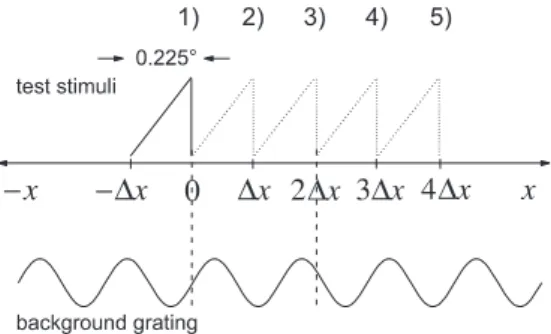
Consider the single sawtooth pattern

S

saw

…x; x

k

† ˆ 1 ‡ …x ÿ x

k

†=Dx; x

k

< x x

k

k ˆ 1; ; 5;

0; else

…9†

with x

k

ˆ …k ÿ 1†Dx, Dx ˆ 0:225 deg. Each of the patterns s

saw

…x; x

k

†, k ˆ 1; . . . ; 5 was employed as a test pattern.

The pattern de®ned for x

1

ˆ 0 will be said to be fo- veally presented; its maximum is in the center of the fovea (x ˆ 0).

The background pattern was de®ned by r

2

ˆ ms

b

…x†

with

s

b

…x† ˆ sin…2pf †; or cos…2pf †

…10†

The grating patterns always subtended the total visible area of 8 8 deg. The relation between test and background pattern is shown in Fig. 2.

Note that s

saw

…x; x

2

† ˆ s

saw

…x ÿ Dx; x

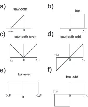
1

†. Let s

saw

…x; x

2

†

def

ˆ

s…I † and de®ne s…II † ˆ

^def

ÿs…I†, s…III † ˆ

^def

s

saw

…ÿ…x‡

Dx††, s…IV † ˆ

^def

ÿs

saw

…ÿ…x ‡ Dx††, see Fig. 3. From these patterns two more stimulus patterns may be de®ned:

s

^even_saw ^def

ˆ s…I† ‡ s…III † and s

^odd_saw^def

ˆ s…I † ‡ s…IV †.

Eventually, stimulus patterns were de®ned either as a single vertical bar or as being composed of bars. Single bars are de®ned either as

s

bar

…x† ˆ 1 for x 2 ‰0; DxŠ; s

t

…x† ˆ 0 otherwise …11†

with Dx ˆ :225 deg; such bars can be composed as a superposition of two sawtooth patterns, see Fig. 4.

Fig. 2. Test stimuli and subthreshold gratings. Test patterns were constructed by shifting the test pattern at x

1

ˆ 0 deg to positions x

k

ˆ …k ÿ 1†Dx, k ˆ 1; . . . ; 5. All ®ve resulting test patterns have the same amplitude spectra, but di€erent phase spectra

5

`deg' is used for `degrees of visual angle'.

Alternatively, patterns composed of bars are de®ned as

s

^even_bar

ˆ 1; x 2 ‰ÿ:5; :5†;

0; otherwise 8 <

: s

^odd_bar

ˆ ÿ1; x 2 ‰ÿ:5; 0†;

1; x 2 …0; :5Š;

0; otherwise 8 <

:

…12†

see Fig. 5.

Thus, s

^even_bar

is a 1 deg wide vertical bar with midpoint at the fovea; since the pattern is even, its spectrum has no imaginary part. s

^odd_bar

, on the other hand, is an odd pattern with its centre at the fovea. The spectrum con- tains no real part.

3.2 Procedure

In order to determine threshold contrasts, a variant of the Method of Limits was employed. This variant may be characterised as follows:

1. The stimulus (either the test stimulus pattern alone or the superposition of the test stimulus pattern plus a background grating) is presented as a sequence of steps, where each step has a duration of 200 m. For given value of m

b

, the sequence is either decreasing or increasing; in a decreasing sequence the contrast m

t

(m

t

ˆ m

0t

if m

b

ˆ 0) is decreased, in an increasing sequence the contrast m

t

is increased after each step until, after a certain step, the subject responds; the response signals that the pattern is no longer seen if

the sequence decreases and that it has been detected if the sequence increases.

2. For ®xed value of m

b

of the background grating, the contrast m

t

of the test pattern was, in a decreasing sequence, reduced by Dm, e.g. Dm ˆ 4:2 10

^ÿ4

, from one step to the next, and increased by the same amount in an increasing sequence.

In a decreasing sequence, the contrast of the pattern in the last step before the subject's response is the lower value / ^

l

. In an increasing sequence, the con- trast of the pattern in the step before the subject's response is the upper value / ^

_u

.

3. Decreasing and increasing sequences were taken in pairs, i.e. a decreasing sequence was followed by an increasing one and an increasing sequence by a de- creasing one. The starting value of the contrast m

t

for an increasing sequence was always m

tl

ÿ :012, where m

tl

is the lower value determined in the pre- ceding decreasing sequence. The starting value for a decreasing sequence after an increasing sequence was, analogously, m

tl

‡ :012, where m

tl

is now the upper value last determined.

4. The estimate U

1

was determined as follows. For the ith pair of sequences, the arithmetic mean / ^

_i

ˆ … / ^

_li

‡ / ^

_ui

†=2 was computed. The estimates ^ a and ^ b are LS-estimates from the pairs …m; /…m†† ^ with /…m† ˆ ^ P

i

/ ^

_i

=8.

To determine U

2

the di€erences D

i^def

ˆ m ^

0t;i

ÿ / ^

_i

, with m ^

0t;i

the estimate of m

0t

in the ith sequence, were determined for a given value of m. The di€erence D ˆ / ^

_k

…m; x† ÿ m ^

0t

in (5) was then estimated as the arithmetic mean D…m† ˆ P

i

D

i

=8.

Fig. 3. Test patterns s

t

generated from the pattern at position x

2

ˆ 0:225 deg. This pattern will also be called s…I†. Mirroring this pattern on the y - axis (contrast) and the x - axis (location) produces the test stimuli s…II†, s…III† and s…IV†

Fig. 4. A bar is given as the superposition of two appropriately chosen sawtooth edges, i.e. s

bar

ˆ s

saw

…ÿx; x

1

† ‡ s

saw

…x; x

2

†

Fig. 5. Overview of the test stimuli used in the experiment. The

sawtooth edge was presented at x

1

ˆ 0 deg and at four further retinal

positions, as shown in Fig. 2. All other stimuli were presented only at

the single position x

1

ˆ 0 deg as shown have. A comparison with

Fig. 3 shows that s

^even_saw

ˆ s…I† ‡ s…III†, s

^odd_saw

ˆ s…I† ‡ s…IV†

The standard deviation of the eight estimates will be used to indicate the estimation error.

3.3. Subjects

Two male persons served as subjects, both corrected myopes and experienced observers, one of them the author G.M. All the data reported were taken by the subject who was naive with regard to the purpose of the experiment; G.M. took only control measurements in order to con®rm the qualitative nature of the curves.

4 Results

4.1 Linear approximation to CIFs

For all stimulus patterns employed in the experiment, a linear approximation of the CIF was determined. We present data in particular for s

saw

…x; x

2

†. Figure 6 shows sections of CIFs and the corresponding linear functions approximating the CIFs for various values of the spatial frequency f ˆ x=2p. The square of the correlation (i.e.

the coecient of determination) between the m

i

and the corresponding estimates /

_t

…m

i

† was generally about :98.

Figure 6a in particular shows CIFs and the linear approximations for s

b

in sine-phase, where the axes show the normalised contrasts m ~ and /, i.e. the ~ x-axis shows m ~ ˆ m=m

0b

with m

0b

the threshold contrast for the grating without the superimposed test pattern, and the y- axis shows / ~ ˆ /…m†= ^ m ^

0t

, m ^

0t

an estimate of the threshold contrast of the test pattern s

t

without the background grating. The overall non-linearity of /…m† is

obvious. For f ˆ 2c=deg, / can be approximated by a linear function /

_t

over (at least) the range …ÿ:5; :5†; for f ˆ 4c=deg, the range of m-values (i.e. of M

t

) is even larger. For this frequency the CIF may be taken to be parallel to the x-axis if the normalised contrast m ~ satis®es ÿ:5 < m ~ < :5, indicating that this frequency has no in¯uence upon the detection of s

saw

…x; x

2

† within the range of background contrasts employed (negative contrasts re¯ect a phase shift of the background grating by 180

⁰

). For values of the normalised contrast in the neighbourhood of 1, however, the CIF becomes almost parallel to the y -axis [representing the normalised contrast of the test-pattern s

saw

…x; x

2

†]. Figure 6b shows the results for the cosine-phase. For the test patterns employed there exists an interval M

t

of normalised contrasts containing m

0t

upon which the linear approx- imation for the CIF holds. Altogether, we may assume that for each of the patterns employed, a corresponding interval M

t

exists upon which detection is by a dominant channel.

4.2 Test of the matched-®lter hypothesis 4.2.1 Matched ®lters at di€erent eccentricities

The hypothesis that a given stimulus pattern is detected by a matched ®lter for this pattern implies that the sensitivities U

i

, i ˆ 1; 2 should re¯ect the spectrum of the pattern. We will present results for the stimulus patterns s

saw

…x; x

k

†, k ˆ 1; . . . ; 5, employing (7) in order to predict especially the sensitivities U

2

corresponding to either the real or the imaginary part of the spectrum of the test pattern s

t

. The test requires the determination of estimates of a

t

jG…f ; x

0k

†j

²

=c, x

0k

ˆ …k ÿ 1†Dx, f ˆ x=2p, for the di€erent values of k. To illustrate, we

Fig. 6a,b. Contrast interrelationship functions in the normalized contrast space. a Recorded for the test pattern s

saw

…x; x

1

†, superimposed on sine gratings. The grating contrasts range from half the negative grating threshold contrast up to the positive threshold contrast for the grating alone.

The curves are shown for two spatial frequencies (s key). Threshold contrast measurements for normalized grating contrasts m ~ greater than 0.5

were obtained by inverting the order of superposition (the gratings were superimposed on test patterns of constant contrast, the subject had to

adjust the contrast for the grating until the compound pattern was at threshold). The linear functions are the regression lines for m ~ 2 ‰ÿ:5; :5Š and

are the linear approximations /

t

to /; negative contrasts refer to background gratings shifted by 180

. b Same test patterns, superimposed upon

cosine gratings well below threshold. The curves were measured only for positive grating contrasts

present the results for the eccentricities 0 and Dx ˆ :225 deg. Figure 7 shows the results, which correspond to those of Hauske et al. (1976): the data indicate a bandpass character of G.

As pointed out in Sect. 2.3.1, the grating sensitivity h

b

, which is, according to (3), proportional to the system function of the detecting channel (provided the pattern is indeed detected by a matched ®lter as speci®ed in Sect.

2.1.5), may be estimated either by U

1

or by U

2

. U

1

re- quires the estimation of the parameters of the linear approximation of the CIF. This is time consuming and necessary only if one wants to explore the range of contrast values for which a linear approximation to the CIF is meaningful. In order to test the hypothesis of detection by a matched ®lter (i.e. assumptions A

1

and A

2

), the estimation of U

2

is more parsimonius. We have tested the equivalence of U

1

and U

2

to make sure that U

2

may be used safely. Figure 8 shows the results of the test of the matched-®lter hypothesis according to (7) for various values of x

k

; Fig. 8b shows the points resulting from estimates U

1

and U

2

, showing the excellent corre- spondence of the two estimates. One may say that within the precision of measurements, the data correspond to the matched-®lter hypothesis.

4.2.2 Crossvalidation I: the e€ect of modulation sign Consider the patterns s…I† and s…II† in Fig. 3. Obviously, s…II† ˆ ÿs…I†, and correspondingly the spectra of the two patterns also di€er just by sign. Figure 9a gives the results for the sine- and Fig. 9b for the cosine- background. For the pattern s…I† the data are compat- ible with the hypothesis of detection by a matched ®lter (c.f. Fig. 8). So if the predictions for s…II† di€er from those for s…I† just by sign we may argue that the pattern s…II† is also detected by a matched ®lter corresponding to this pattern.

Clearly, the sensitivity curves are mirror images of each other, supporting the hypothesis of detection by a matched ®lter for s…II†. Moreover, the results imply that we may assume that a

t

jG…x; x

0

†j

²

=c has the same value for s…I† and s…II†.

4.2.3 Crossvalidation II: even and odd compound patterns As already noted by Kulikowski and King-Smith (1973), Shapley and Tolhurst (1973) and Hauske et al. (1976), even test patterns are only a€ected by cosine-type gratings, and odd test patterns only interfere with sine- type gratings.

Let us consider the patterns s

^odd_t

ˆ s…I† ‡ s…IV† and s

^even_t

ˆ s…I† ‡ s…III† (referred to as ``sawtooth-odd'' and

``sawtooth-even'', respectivley, in Fig. 5), where s…I†, s…III† and s…IV† are as de®ned in Fig. 3, Sect. 3.1.2 Let S

_t^odd

and S

_t^even

be the Fourier transforms of s

^odd_t

and s

^even_t

, and let S

t

be the Fourier transform of s

t

ˆ s…I†. We ®nd that S

_t^odd

2Im…S

t

†, S

_t^even

2Re…S

t

†.

The data for s

^odd_t

are presented in Fig. 9c, those for s

^even_t

in Fig. 9d. The sensitivity estimates for s…I† and s

^odd_t

ˆ s…I† ‡ s…IV† for sine-background and s…I† and s

^even_t

ˆ s…I† ‡ s…III† for cosine-background agree as predicted by the matched-®lter model, but the sensitivity estimates do not di€er by a factor of 2. Now the size of the retinal area covered by each of the patterns s…I† to s…IV† is identical, and for reasons of symmetry we may assume that a

t

jGj

²

=c assumes the same value for the four stimulus patterns. However, s

^odd_t

and s

^even_t

cover twice the area covered by an individual pattern. This may well mean that the values of a

t

of the patterns s…I† to s…IV†

di€er from the values of a

t

for the compound patterns, and consequently the estimates of a

t

jGj

²

=c will di€er. It follows that one cannot expect the sensitivity estimates for s

^odd_t

and s

^even_t

just to di€er by a factor of 2 (or 1/2).

4.2.4 Crossvalidation III: bar patterns

Stimulus patterns may in principle be represented as linear superpositions of some other, appropriately chosen patterns. For instance, consider a vertical, rectangular bar. The bar is the sum of two sawtooth patterns s

bar

ˆ s

saw

…ÿx; x

1

† ‡ s

saw

…x; x

2

† (see Fig. 4), and the spectrum of the bar pattern equals the sum of the spectra of the sawtooth patterns; we denote the sawtooth pattern by s

saw

. Suppose that the bar-pattern is again detected by a matched channel for a bar of width Dx and position as de®ned in (11); then the (grating) sensitivity of the bar

Fig. 7a,b. Values of a

t

jGj

²

=c, estimated according to (6) (®lled squares), estimates based on U

^cos₂

(®lled circle), U

^sin₂

(open triangles), for stimulus

patterns at x

1

ˆ 0 deg and x

2

ˆ :225 deg, exhibiting band pass character. A third-order polynomial was ®tted to represent all estimates (solid line)

Fig. 8a±e. Sensitivity functions U

2

…f †, f ˆ x=2p, for sawtooth patterns s

saw

…x; x

k

†, k ˆ 1; . . . ; 5; for background gratings in sine- (open triangles)

and cosine-phase (®lled circles). Solid and dashed curves are the predictions of the matched ®lter model. b additionally shows estimates based on

U

1

. Apparently missing open symbols are due to the fact that they represent data coinciding with the corresponding prediction. See text for further

explanation

channel should be predicted by the sum of the corre- sponding sensitivities of the two sawtooth patterns.

Figure 10 shows the sensitivities, as measured for the bar (®lled circles), for cosine- (a) and sine-gratings (b).

The data are certainly compatible with the hypothesis of detection by a matched ®lter for this pattern. The open triangles in Fig. 10a,b are the predictions from the sum of the sensitivities of the two sawtooth patterns after multiplication by a factor a

0

2=3. The correspondance to the direct measurements for the bar is very good, ÿ however, the price to be paid is the introduction of the factor a

0

. One reason for having to introduce this factor could be that the factors a

t

for bar pattern on the one hand and sawtooth patterns on the other (or their cor- responding channels) di€er.

Figure 11a shows the data and corresponding pre- dictions of the matched ®lter model for a bar of width Dx ˆ :225

⁰

at position x

1

ˆ :00 (see Fig. 5b); the ®lled circles represent the measurements for the cosine-back- ground grating, the open triangles those for the sine- background grating. The data are obviously compatible

with the hypothesis of detection by a matched ®lter for the bar pattern.

Figure 11b contains the measurements and the cor- responding prediction of the matched ®lter model for (i) Dx ˆ 1

⁰

bar (``bar-even'' in Fig. 5); since the pattern is even there are only measurements for s

b

in cosine-phase (®lled circles), and (ii) for a bar pattern also of Dx ˆ 1

⁰

width (``bar-odd'' see Fig. 5) with s

b

just in sine-phase since the pattern is odd. For the ``bar-even'' pattern the data correspond to the predictions. This cannot be said for the ``bar-odd'' pattern. In order to exclude the pos- sibility of faulty experimenting, the measurements were repeated at other times with di€erent subjects; however, the result remains the same and may therefore be con- sidered as systematic.

5. Discussion

We have presented data that are compatible with the matched ®lter model at least to some extent. Brie¯y, the

Fig. 9a. Sensitivity functions, for positive (®lled circles) and negative (open triangles) modulations of the test stimulus for sine and b cosine

background gratings. The corresponding stimulus pattern is given in the key. c, d Sensitivity functions for the same test stimulus (®lled circles). c

In addition, the pure odd stimulus s

^odd_saw

ˆ s

saw

…I† ‡ s

saw

…IV† (open triangles, s, key of Fig. 3), superimposed on sine gratings. d Sensitivity functions

for the test pattern (®lled circles) and the pure even test pattern s

^even_saw

ˆ s

saw

…I† ‡ s

saw

…III† (open triangles), for cosine background gratings

model ®ts the data well if the stimulus pattern (i) covers a relatively small retinal area (here: .225 deg), and (ii) shows a de®nite `feature' (here: an edge, de®ned by the sawtooth luminance distribution de®ned in Sect. 3.1.2, or two edges as found with the vertical bar of .225 deg width). The data conform with the model not only for a

®xed position, e.g. the fovea, but also if the stimulus pattern is presented at di€erent foveal positions.

There are some open questions, though. One refers to the factor a

t

, introduced in (1) as a free parameter. If the system function of a matched ®lter is derived from a decision theoretical point of view (e.g. Peterson et al.

1954; Whalen 1971) one is led to the postulate that the impulse response h of the ®lter should be given by h…x† ˆ s…x

^‡₀

ÿ x†, s the stimulus to which the ®lter is matched, and x

^‡₀

the point of maximal response. This means that h is de®ned not only with respect to the form of s, but also with respect to its modulation. If we

consider instead of s the pattern ms, m some real number representing contrast, the corresponding matched ®lter should be de®ned by mh. Clearly, the energy of s di€ers from that of ms. The factor a

t

enters to account for the appropriate adjustment of the energy of the signal to which the ®lter is matched. So, if in particular s

t

has unit contrast and the presented stimulus is ms

t

, we would have to put a

t

ˆ m. This is the approach of Hauske (1988), who argued that if in particular the stimuli are presented with threshold contrasts m

0t

, one should have a

t

ˆ m

0t

. Although this assumption is plausible, we have not explicitly incorporated it. Firstly, if one assumes that matched ®lters exist as ®xed units within the visual system, one would have to postulate that they also exist for di€erent modulations of the same s; however, this seems to be a very wasteful way of wiring the system. If, on the other hand, one assumes that matched ®lters are formed, e.g. as a result of detection tasks, they will be

Fig. 10a,b. Predicting the sensitivities for a bar pattern from those for sawtooth patterns. Solid line: prediction of the matched-®lter model, a sine- grating, b cosine-grating. The factor a

0

was found to be close to 2/3

Fig. 11a. Sensitivity estimates U

2

…f †, f ˆ x=2p, for a bar pattern Dx ˆ 0:225 deg wide (see Fig. 5b) presented at x

1

ˆ 0:0 deg (®lled circles,

cosine-background; open triangles, sine-background). b Sensitivity estimates U

2

…f † for s

^even_bar

(see Fig. 5e), superimposed on cosine gratings (®lled

circles), and s

^odd_bar

(see Fig. 5f), superimposed on sine-gratings (open triangles), each with width Dx ˆ 1 deg. Dashed and solid lines are the

predictions of the matched ®lter model

formed with respect to the modulation actually occur- ring. However, the modulation varies between trials as a result of the fact that either m

0t

± when there is no background grating ± or /…m† has to be determined experimentally (cf. Section 2). Possibly a

t

will assume values near to the true value of m

0t

, but whether this is indeed so is an additional hypothesis that has to be tested. On the other hand, our main aim was to test the hypothesis of the existence of matched ®lters, and with respect to this hypothesis, it is sucient to test for the proportionality to the spectra of the test stimuli of the sensitivities U

i

, i ˆ 1; 2. We therefore decided not to suggest particular values of a

t

.

The model does not ®t for the bar-odd pattern s

^odd_bar

of 1

⁰

width (see Fig. 11b). One may speculate that di€erent matched ®lters ± e.g. one for the bright and one for the dark bar ± compete in the detection process, meaning that processes of attentional focussing may play a role in this process. Further research is necessary here. Also, for s

^odd_saw

and s

^even_saw

the data correspond qualitatively, but not in a strict, quantitative sense to the predictions of the matched ®lter model. These ®ndings clearly restrict the generality of the matched ®lter model; since the model is supported for the smaller stimulus patterns, one may speculate that matched ®lters exist or form only for ®ner details; for related results, cf. Hauske et al. (1978).

Again, further research is needed here.

We argued that dominance of the detecting channel C

l

± provided the stimulus pattern is indeed detected by a single channel ± has to be an essential feature of C

l

if its characteristics are to be explored by the superposition method. Since for the smaller patterns the matched ®lter model is compatible with the data, one may argue that the detecting ®lters are dominant.

It is possible that certain subsystems of the visual system exist like the receptive ®elds (RFs) considered by Koenderink and van Doorn (1990) which could act like matched ®lters for appropriately chosen stimulus pat- terns. However, no such receptive ®eld is likely to dominate the detection process simply because many functionally similar RFs exist, possibly arranged in a stack, and the overlap of activities of these RFs will imply some sort of pooling, probabilistic or otherwise, of their responses. In cases like this, the superposition method cannot reveal the matched ®lter properties of the RFs even if the RFs had this property (Mortensen et al., unpublished manuscript). An argument of this sort may also apply to Logvinenko's (1993) failure to demonstrate the matched ®lter property for spatial frequency chan- nels; his data may also be contaminated by a bias of the sort discussed in Sect 2.3, comment 2.

The question of whether the superposition method allows us to identify matched ®lters under any circum- stances also arises when another class of models is considered. For instance, von der Heydt, Peterhans and Baumgartner (1984) suggested a computational model of form processing incorporating cortical simple, com- plex and end-stopped cells, and Heitger, Rosenthaler, von der Heydt, Peterhans and KuÈbler (1992) showed how cortical simple, complex and end-stopped cells may cooperate to allow for the perception of complicated

contours. The notion of a matched ®lter is not intro- duced in these models; however, with respect to the al- ready mentioned work of Oja (1982) and Nachtigall (1991), one may speculate that networks of simple, complex and end-stopped cells exist behaving like mat- ched ®lters for certain features. If, however, the subject's attentional focus can oscillate between di€erent ®lters, the superposition method will yield a blurred picture of them which seemingly contradicts the matched ®lter hypothesis. The apparent breakdown of the matched

®lter model reported by Hauske et al. (1978) may be due to this fact. A more detailed discussion of this possibility is, however, beyond the scope of this paper.

It should be mentioned that Logvinenko (1995, 1996) takes a di€erent path in order to interpret the ®ndings from superposition experiments; he tries to derive the properties of channels from the convexity of CIFs. Since probability summation among channels does not seem to play a role in his model ± at least he has not treated probability summation explicitly ± his conclusions about the meaning of gradients of CIFs at m

b

ˆ 0 di€er from ours.

In any case, threshold curves generated by the su- perposition method may be distorted by processes of quite a di€erent sort: HuÈbner (1993) has argued that shifts of attention may even alter the tuning of spatial frequency channels, and attentional processes usually remain rather uncontrolled in experiments of the type reported here. It is possible that the psychophysical ex- ploration of channels of the visual system ± provided such entities exist at all ± cannot be achieved, disre- garding the cognitive aspects of stimulus detection.

References

Beard BL, Levi DM, Reich LN (1995) Perceptual learning in pa- rafoveal vision. Vision Res 35:1679±1690

Daugman JG (1984) Spatial visual channels in the Fourier plane.

Vision Res 24:891±910

Du Buf JMH (1993) Responses of simple cells: events, interfer- ences, and ambiguities. Biol Cybern 68:321±333

Du Buf JMH (1992) Modeling spatial vision at the threshold level.

Spatial Vision 6:25±60

Du Buf JMH (1994) Ramp edges, Mach bands, and the functional signi®cance of the simple cell assembly. Biol Cybern 70:449±461 Gardiner CW (1990) Handbook of stochastic processes for physics, chemistry and the natural sciences. Springer, Berlin Heidelberg New York

Graham N (1977) Visual detection of aperiodic spatial stimuli by probability summation among narrowband channels. Vision Res 17:637±652

Graham N (1980) Spatial ± frequency channels in human vision:

detecting edges without edge detectors. In: Harris CS (ed) Vi- sual coding and adaptability. Lawrence Erlbaum, Hillsdale Graham N (1989) Visual pattern analyzers. Oxford University

Press, Oxford

Hauske G, Wolf W, Lupp U (1976) Matched ®lters in human vi- sion. Biol Cybern 22:181±188

Hauske G, Lupp U, Wolf W (1978) Matched ®lters. A new concept in vision. Soc Photogr Sci Eng 20:59±64

Hauske G (1988) The visual system as a spatial frequency matched

®lter. In: Marko H, Hauske G, Struppler A (ed) Processing

structures for perception and action. Final report of the Son-

derforschungsbereich `Kybernetik' 1969±1983, Weinheim

Hebb DO (1949) The organisation of behavior. Wiley, New York Heitger F, Rosenthaler L, Heydt R von der, Peterhans E, KuÈbler O (1992) Simulation of neural contour mechanisms: from simple to end-stopped cells. Vision Res 32:963±981

Hertz J, Krogh A, Palmer RG (1991) Introduction to the theory of neural computation. Addison-Wesley, Reading, Mass Heydt R von der, Peterhans E, Baumgartner G (1984) Illusory

contours and cortical neuron responses. Science 224:1260±

Hines M (1976) Line spread variation near the fovea. Vision Res 1262 14:567±572

Hsu HP (1970) Fourier analysis. Simon &Schuster, New York HuÈbner R (1993) Di€erent ways of modeling spatial-frequency

uncertainty in visual signal detection. Biol Cybern 69:457±462 Jaschinski-Kruza W, Cavonius CR (1984) A multiple channel

model for grating detection. Vision Res 24:933±941

Kendall MG, Stuart A (1969) The advanced theory of statistics, Vol 1. Grin, London

Kendall MG, Stuart, A (1973) The advanced theory of statistics, Vol 2. Grin, London

Kirkwood A, Rioult M, Bear MF (1996) Experience-dependent modi®cation of synaptic plasticity in visual cortex. Nature 381:526±528

Koenderink JJ, Doorn AJ van (1990) Receptive ®eld families. Biol Cybern 63:291±297

Kulikowski JJ, King-Smith PE (1973) Spatial arrangement of line, edge and grating detectors revealed by subthreshold summa- tion. Vision Res 13:1455±1478

Logvinenko AD (1993) Lack of convexity of threshold curves for compound grating: implications for modelling visual pattern detection. Biol Cybern 70:55±64

Logvinenko AD (1995) On deriving analyser characteristics from summation-at-threshold data. Biol Cybern 73:547±552 Logvinenko AD (1996) Convexity of a set of subthreshold stimuli

implies a peak detector. Spatial Vision 10:105±123

Nachtigall C (1991) Modellierung eines selbstorganisierten Mat- ched-Filters durch ein System gewoÈhnlicher Di€erential- gleichungen. Diplomarbeit am Fachbereich Mathematik der Westf. Wilhelms-UniversitaÈt MuÈnster

Oja E (1982) A simpli®ed neuron model as a principal component analyzer. J Math Biol 15:267±273

Papoulis A (1981) Systems and transforms with applications in optics. Robert E. Krieger, Malabar

Peterson WW, Birdsall TG, Fox WC (1954) The theory of signal detectability. Trans IRE Professional Group in Information Theory, PGIT 2-4, 171-212, Reprint in: Luce RD, Bush RR, Galanter E (ed) (1963) Readings in mathematical psychology, Vol. 1. John Wiley and Sons, New York

Poggio T, Fahle M, Edelman S (1992) Fast perceptual learning in visual hyperacuity. Science 256:1018±1021

Ross JR, Morrone MC, Burr DC (1989) The conditions under which Mach bands are visible. Vision Res 29:699±715 Sachs MB, Nachmias J, Robson JG (1971) Spatial frequency

channels in human vision. J Opt Soc Am 61:1176±1186 Shapley RM, Tolhurst DJ (1973) Edge detectors in human vision.

J Physiol 229:165±183

Watson AB (1982) Summation of grating patches indicates many types of detector at one retinal location. Vision Res 22:17±25 Wilson HR, Bergen JR (1979) A four mechanism model of

threshold spatial vision. Vision Res 19:515±522

Wilson HR, Giese SC (1977) Threshold visibility of frequency

gradient patterns. Vision Res 17:1177±1190