importance of the pelagic polychaete Poeobius sp. in the tropical Atlantic
Master Thesis in Biological Oceanography
submitted by
Svenja Christiansen
(6100)
Kiel 31st October 2016
Examined by:
Prof. Dr. Thorsten Reusch Supervised by:
Dr. Henk-Jan T. Hoving & Dr. Rainer Kiko
[1] [2]
Declaration of authorship
Hiermit erkläre ich, dass ich die vorliegende Arbeit selbstständig geschrieben habe und keine anderen als die ausgewiesenen Quellen zur Hilfe genommen habe. Diese Masterarbeit wurde in keinem anderen Prüfungsverfahren eingereicht. Die gedruckte Version entspricht der auf einem elektronischen Datenträger gespeicherten. Mit einer Veröffentlichung in der Bibliothek des GEOMAR und in der Zentralbibliothek der Christian-Albrechts-Universität bin ich einverstanden.
Hereby I certify that this Master thesis is my own work and no other than the declared references were used. This thesis has not been in any other examination procedure. The printed version is consistent to the version provided on a digital data carrier.
Kiel, 31.10.2016
Zusammenfassung
Die Verbreitung und Rolle von gelatinösem Zooplankton im ausgedehnten Lebensraum des pelagischen Ozeans ist weitgehend unbekannt und es werden immer noch neue Arten und neue ökologische Zusammenhänge entdeckt.
Gelatinöses Zooplankton wird auf Grund seiner empfindlichen Struktur während des Fanges mit Netzen oft beschädigt, daher wurde diese sehr vielfältige Gruppe lange unterschätzt. Erst die Entwicklung von Unterwasserkameras machte die quantitative Erfassung dieser Organismen möglich. Im Jahr 2015 wurden während eines Einsatzes einer geschleppten Videokamera (PELAGIOS) im tropischen Atlantik hohe Abundanzen eines holopelagischen Polychaeten der Gattung Poeobius in einem mesoskaligen Eddy entdeckt. Außerdem wurden in diesem Wirbel sehr geringe Partikelkonzentrationen festgestellt. Bisher ist nur eine Art dieser Gattung, Poeobius meseres, im pazifischen Ozean bekannt. Dort wurde eine Abhängigkeit zwischen hoher Polychaetendichte und abnehmenden Partikelkonzentrationen beschrieben.
Mehrere Veröffentlichungen betonen die Wichtigkeit des Meso- und Makrozooplanktons in der Remineralisation von Partikeln in den oberen 100 m der Wassersäule, aber es ist wenig darüber bekannt, welchen Einfluss gelatinöse Partikelfresser auf den Partikelfluss in mesoskaligen Eddies haben. Nach der ersten Beobachtung von Poeobius sp. im tropischen Atlantik in dem PELAGIOS Video wurde der Polychaet auch auf Bildern des Underwater Vision Profilers (UVP5) identifiziert. Der UVP5 ist eine hoch auflösende Kamera, welche sowohl Partikel als auch Meso- und Makrozooplankton quantitativ aufnimmt.
In dieser Arbeit nutze ich UVP5- und Umweltdaten von 13 Forschungsfahrten im tropischen Atlantik mit über 1.8 Millionen Bildern, um die horizontale und vertikale Verbreitung von Poeobius sp. zu charakterisieren. Ich teste die Hypothese, dass Poeobius sp. Eddy-assoziiert ist und untersuche die möglichen Auswirkungen hoher Abundanzen auf die Biogeochemie von Eddies. Insgesamt wurden 481 Individuen zwischen 5°S und 20°N und 16°W bis 46°W beobachtet, mit einer Mindesttiefe von 22 m und einer maximalen Tiefe von fast 1000 m. Ein Vergleich von verschiedenen Eddytypen sowie Stationen außerhalb von Eddies zeigte eine erhöhte Abundanz und eine eingeschränkte Tiefenverteilung von Poeobius sp. in antizyklonischen mode- water Eddies ('anticyclonic mode-water eddies', ACMEs). Die Ergebnisse dieser Arbeit suggerieren, dass Eddies, insbesondere ACMEs, einen Mechanismus für die Vermehrung und die Verbreitung von sonst seltenem Zooplankton darstellen können. Diese können wiederum die Umweltbedingungen im Eddy beeinflussen:
Zum Beispiel konnten hohe Poeobius sp. Abundanzen mit sehr geringen
Partikelkonzentrationen und Partikelflüssen in den unmittelbar darunter befindlichen Schichten in Verbindung gebracht werden. Der Partikelfresser Poeobius sp. könnte durch ausgedehnte Schleimnetze einen wesentlichen Teil des vertikalen Partikelflusses aufnehmen. Insbesondere in mesoskaligen Eddies könnten diese Prozesse eine wichtige Rolle in der Entwicklung von Partikelflüssen spielen. Diese Ergebnisse sollten bei der Diskussion und Modellierung der Ökologie und Biogeochemie von Eddies berücksichtigt werden. Sie betonen die Wichtigkeit optischer Methoden für die Erfassung von ökologischen Zusammenhängen im pelagischen Ozean.
Abstract
The distribution and ecological function of gelatinous zooplankton in the vast habitat of the pelagic oceans is mostly unknown and new species and their roles in the ecosystem are still being discovered. Nets undersample and destroy this highly diverse group of organisms, thus, the use of underwater optical systems is the most appropriate way to observe them. In 2015, the deployment of the towed pelagic in situ video camera system (PELAGIOS) revealed high abundances of a holopelagic polychaete of the genus Poeobius in a mesoscale eddy in the tropical Atlantic, where it co-occurred with very low particle concentrations. Its sister species, the flux-feeder Poeobius meseres, is only known from the Pacific Ocean. A negative correlation of the polychaete with particle concentrations was described there. Several publications emphasize the role of mesozooplankton in remineralisation, but little is known about the impact of gelatinous particle-feeders on the flux in mesoscale eddies. After the discovery of Poeobius sp. in the Atlantic by PELAGIOS, it was also identified on images of the Underwater Vision Profiler 5 (UVP5), a high-resolution camera that quantitatively records both particle concentrations and mesozooplankton. Here I use UVP5 and environmental data, including more than 1.8 million images from 13 cruises, to identify the horizontal and vertical distribution of Poeobius sp. in the tropical Atlantic Ocean. I test the hypothesis that Poeobius sp. is associated with mesoscale eddies and investigate its biogeochemical role in these features. In total, 481 individuals were observed between 5°S and 20°N and between 16°W to 46°W with the shallowest observation at around 22 m and the deepest at around 1000 m depth. A comparison between non-eddy stations and three different eddy types revealed elevated abundances and a restricted depth distribution of Poeobius sp.
especially in anticyclonic mode water eddies (ACMEs), confirming the hypothesis of eddy association. The results from this thesis suggest that mesoscale eddies, especially ACMEs, may serve as an aggregation and dispersal mechanism for Poeobius sp. and possibly other low-oxygen tolerant zooplankton species. These in turn influence the environment of the eddy: High Poeobius sp. abundances could be related to strongly reduced particle concentrations and fluxes in the layers directly below the polychaetes. It is shown that the worms take up almost the entire vertical particle flux by feeding with their mucus nets. Poeobius sp. may play a significant role in the development of particle fluxes, and thus the biological carbon pump, in ageing mesoscale eddies. These results should be considered when discussing or modelling mesoscale eddy ecology and biogeochemistry.
Contents
Declaration of authorship 2
Zusammenfassung 4
Abstract 6
Contents 7
1 Introduction 10
1.1 Biogeochemistry in the upper ocean 10
1.2 Zooplankton and its role in the biological carbon pump 10
1.3 The flux-feeder Poeobius sp. 11
1.4 Sampling bias and the need for optical methods 12
1.5 Influence of oceanographic features on zooplankton distribution and particle flux, and
the role of mesoscale eddies 12
1.6 Scope 14
2 Data and Methods 15
2.1 The Underwater Vision Profiler and PELAGIOS 15
2.2 Study area 16
2.3 Environmental data 18
2.4 Assignment of profiles to eddy and shelf 19
2.5 Assessment of Poeobius sp. abundance and depth 20
2.5.1 Image sorting 20
2.5.2 Size determination 21
2.5.3 Calculations and binning 22
2.6 Assessment of particle concentrations, sizes and flux 24 2.7 Calculation of Poeobius sp. respiration and carbon utilisation 25
2.8 Comparison of UVP5 and PELAGIOS counts 26
2.9 Statistics 26
2.9.1 Comparisons between eddy and non-eddy stations 26
2.9.2 Generalized linear mixed model 27
3 Results 28
3.1 Poeobius sp. distribution and eddy association in the tropical Atlantic 28
3.1.1 Horizontal distribution 28
3.1.2 Vertical distribution 31
3.1.3 Distribution in relation to environmental factors 34
3.1.4 Poeobius sp. length 37
3.2 Implications of high Poeobius sp. abundances on the particle abundance and
biogeochemistry of mesoscale eddies 38
3.2.1 Observations of feeding behaviour 39
3.2.2 Implications on the biogeochemistry of eddies 41 3.2.3 Other zooplankton in E1, E2 and the background 48
3.3 Comparison between UVP5 and PELAGIOS 51
3.3.1 Relationship between counts of the different instruments 51 3.3.2 Additional observations from PELAGIOS videos 52
4 Discussion 53
4.1 Advantages and disadvantages of the UVP5 and PELAGIOS 53 4.2 Poeobius sp. distribution in the tropical Atlantic 54 4.2.1 Horizontal and vertical distribution and relation to water masses 54
4.2.2 Reasons for the recent discovery 56
4.3 Comparison of the Atlantic Poeobius sp. with P. meseres 57
4.4 Eddy association of Poeobius sp. 58
4.4.1 Poeobius sp. abundance in eddies 58
4.4.2 Poeobius sp. depth distribution in eddies 61
4.4.3 Differences between the eddy types 62
4.5 Implications on the biogeochemistry of mesoscale eddies 62
4.5.1 Influence of flux-feeders on particle flux 63
4.5.2 Patterns in eddies with high Poeobius sp. abundances 63 4.5.3 Relation of Poeobius sp. to the observed particle patterns 66
5 Conclusion and outlook 69
6 Acknowledgements 70
7 References 71
7.1 Literature 71
7.2 Web pages 77
7.3 Images 77
Appendix i
Supplement 1: i
Supplement 2: ii
1 Introduction
The pelagic ocean is the largest and least explored ecosystem on earth (Ramirez- Llodra et al. 2010). Its communities include planktonic organisms that no one has ever seen until the use of underwater camera systems. One example is the polychaete Poeobius sp., which was not known from the Atlantic until recently. This study explores its distribution in the tropical Atlantic and its potential impact on biogeochemical processes in mesoscale eddies.
1.1 Biogeochemistry in the upper ocean
Anthropogenic greenhouse gas emissions, such as CO2, have lead to global climate change with significant consequences for ocean ecosystems, such as ocean warming, deoxygenation and acidification. This makes the understanding of processes that remove CO2 from the atmosphere necessary. The ocean is an important buffering system for the climate. It is the biggest carbon store on earth with 38000 GT C; in contrast the atmosphere only holds 762 GT (Bollmann et al. 2010). Large amounts of CO2 are fixed at the oceans surface by phytoplankton and thus get introduced into the marine food web. Although most of this surface production never leaves the upper 100 m due to fast remineralisation (Martin et al. 1987), a still considerable amount (2.47 GT y-1 in total for the Atlantic Ocean alone; Antia et al. 2001) is transported into deeper layers in the form of small to large particles (diatom frustules, leftovers of small crustaceans, marine snow, fecal pellets and other detritus) and thus represents an important way of carbon sequestration and one major process of the biological carbon pump (Longhurst and Harrison 1989; Karakaş et al. 2009; Durkin et al. 2015). The actual carbon export to the deep ocean depends on the dynamics and types of planktonic processes in the water column.
1.2 Zooplankton and its role in the biological carbon pump
The oceanic ecosystem is inhabited by a large diversity of heterotrophic organisms ranging from protists to large nekton predators. Among these, zooplankton make up 51% (Gasol et al. 1997) of open ocean biomass. Within this extremely diverse group, organisms show wide ranges of sizes, morphology, behaviour and distribution.
Zooplankton is a key link between primary production and higher trophic levels in the marine food web by feeding on phytoplankton and being fed upon by larger animals (Banse 1995).
Zooplankton is known to contribute to the biological carbon pump by producing fast-sinking particles (fecal pellets and dead bodies (Wilson et al. 2013)) and by performing diel vertical migrations (DVM), i.e. feeding at the surface at night and excreting at depth during the day (Turner 2015). On the other hand, sinking particles are also utilised by many of these animals. There are two basic feeding modes for particle-feeding zooplankton: Filter feeding, which is well described for salps (e.g.
(Hamner et al. 1975) and copepods (Kiørboe 2000), and flux-feeding, which is known for example from pteropods, polychaete larvae and adult polychaetes (Hamner et al.
1975; Jackson 1993; Uttal and Buck 1996; Stemmann et al. 2004; Jackson and Checkley 2011; Turner 2015). Flux-feeders deploy net-like mucus structures on which they collect sinking particles (Gilmer 1974; Hamner et al. 1975). Jackson (1993) distinguishes clearly between filter-feeding and flux-feeding as two different modes, as the former is dependent on particle size and concentration, whereas the latter is independent from particle size, but dependent on particle flux (i.e. the amount of sinking particles per unit time). Iversen (2010) point out the importance of flux- feeding zooplankton for the degradation of particles off Cape Blanc and indicate flux-feeding to be an important process of carbon removal from sinking organic matter in that region: The authors calculated that zooplankton flux feeding was responsible for about 90% of the degradation of particles in particle size classes larger than 1 mm in the upper ocean. Jackson (1993) calculated the influence of pteropods on particle flux by formulating the cross-sectional impact of these animals' mucus web on falling particles and found a median loss of 26% flux by two species alone in the upper 100 m of five different regions of the Atlantic Ocean .
1.3 The flux-feeder Poeobius sp.
In the eastern Pacific Ocean, high abundances of the flux-feeding gelatinous polychaete Poeobius meseres (Heath 1930) were found to significantly increase the light transmission, indicating a decrease in particle concentrations, in the respective depth layer (Robison et al. 2010). Poeobius meseres is a fragile gelatinous worm of up to 2.7 cm length. The holopelagic polychaete of the family Flabelligeridae (Burnette et al.
2005) either catches particles by deploying a mucus net or by grasping single particles with its tentacles (Uttal and Buck 1996). It has a very low metabolism (Thuesen and Childress 1993). Poeobius meseres has been known in the Pacific Ocean for more than 80 years, and the genus was thought to be endemic to that ocean (McGowan 1960), however we only recently discovered an organism belonging to the same genus in the eastern tropical North Atlantic (ETNA) when using underwater imaging systems.
1.4 Sampling bias and the need for optical methods
Zooplankton research has been focussed on hard-bodied, robust animals, especially crustaceans (Robison 2004; Quéré et al. 2005), for a long time. The implementation of optical methods like underwater photography and video led to the discovery that the fragile gelatinous zooplankton (including e.g. medusae, ctenophores, salps, siphonophores and more) is largely undersampled by conventional plankton nets (Remsen et al. 2004; Robison 2004). A time series of ROV video transects revealed the substantial carbon transport to the deep sea by discarded larvacean houses (Robison et al. 2005). Biard et al (2016) performed the first global assessment of the distribution and biomass of large rhizarians, including phaeodaria, radiozoa and foraminifera, by analysing the global image database of the Underwater Vision Profiler (UVP5), which records both particles and mesozooplankton. The authors pointed out the high biomass of rhizaria in comparison to the mesozooplankton biomass known from net catch data, especially in tropical and subtropical oceans and in upwelling regions. In 2015, the deployment of a towed video camera system (pelagic in situ observation system, PELAGIOS) lead to the discovery of high abundances of the flux-feeding polychaete Poeobius sp. in a mesoscale eddy in the tropical Atlantic. These examples show that many aspects of marine zooplankton are still to be investigated, and that the use of optical methods is a key for this. The bias of current biogeochemical models towards crustacean zooplankton (Stemmann et al. 2004; Quéré et al. 2005) can only be overcome with a better knowledge of fragile zooplankton species distributions and their functions in the ecosystem.
1.5 Influence of oceanographic features on zooplankton distribution and particle flux, and the role of mesoscale eddies
The distribution of zooplankton in the three dimensional habitat of the world's oceans is patchy (Davis et al. 1992b). It is determined by biological processes (Folt and Burns 1999), but also by small- to large-scale oceanographic processes, for example mixing, upwelling, downwelling and the distribution of water masses (Martin 2003). Features like oceanic fronts (Fernández and Pingree 1996; Stemmann et al. 2008; Prants et al. 2014), seamounts (e.g., (Boehlert and Genin 1987; Denda and Christiansen 2013) and eddies (Ring 1981; Tsurumi et al. 2005; Stemmann et al. 2008;
Godø et al. 2012; Löscher et al. 2015; Waite et al. 2015; Hauss et al. 2016) play an important role in zooplankton aggregation and dispersal.
Mesoscale eddies are prominent features in the ocean. In the eastern tropical North Atlantic they have recently gained attention due to their strong impacts on physical,
biological and biogeochemical processes in this otherwise oligotrophic region.
Physical processes such as upwelling in the core or around the margins of mesoscale eddies (Karstensen et al. 2016) lead to increased nutrient input and influence surface primary productivity (Oschlies 2002; Sweeney et al. 2003; Godø et al. 2012; Stramma et al. 2013; Löscher et al. 2015) and in the following also to enhanced secondary production (Godø et al. 2012; Hauss et al. 2016), particle production (Sweeney et al.
2003; Waite et al. 2015; Fiedler et al. 2016; Fischer et al. 2016) and oxygen consumption (Karstensen et al. 2015; Waite et al. 2015; Fiedler et al. 2016). Eddies can have different origins: They can spin off coastal boundary currents and, transporting an enclosed water mass across the shelf, propagate into the open ocean (Mackas and Galbraith 2002; Whitney and Robert 2002; Waite et al. 2015; Schütte et al. 2016a). Also, eddies can be generated in the leeward of islands (leeward eddies; e.g. Seki et al. 2002).
Another possible origin of eddies is the generation through disturbance by internal waves or underlying topography in the open ocean (J. Karstensen, GEOMAR, personal communication), but only little is known about these open ocean eddies.
Three types of eddies are discriminated: 1. anticyclones (AC), 2. cyclones (CE) and 3.
anticyclonic mode-water eddies (ACME; McGillicuddy et al. 2007; Schütte et al.
2016a). While 'normal' anticyclones are often less productive than the surrounding water due to downwelling in the eddy core, cyclones and anticyclonic mode-water eddies are known as 'oases in the desert' (Godø et al. 2012).
Are eddies also 'oases in the desert' for flux feeding organisms such as Poeobius sp.?
Eddies can be seen as natural mesocosms as they transport an enclosed water mass with different properties than the surrounding waters (Ring 1981). Processes in these isolated features, like for example, the biological pump working at a different pace (Romero et al. 2016), provide different conditions for life inside the eddy than outside. Increased particle fluxes (e.g.: Fiedler et al. 2016) would suggest eddies to be a favourable habitat for particle-feeding organisms. Additionally, low oxygen conditions, as reported from several mesoscale eddies in the study region (Karstensen et al. 2015; Hauss et al. 2016; Schütte et al. 2016c), may exclude predators with a high oxygen demand (Hauss et al. 2016). The special properties of eddies have been known for many years (Ring 1981), and some work has been done to describe the impact of gulf stream cold- and warm-core rings on the ecosystem. Examples are also known from the Pacific Ocean: Tsurumi et al (2005) described increased pteropod densities in so-called Haida eddies compared to background conditions in the Alaska Gyre. They relate the higher abundances to more favourable conditions (warmer water than the surrounding sub-polar gyre) but do not go into detail about relations to particle concentrations and possible enhanced food availability. Tsurumi et al (2005) and others (Mackas and Galbraith 2002; Mackas et al. 2005) found eddies
of different stage and distance to the coast having a different composition of coastal and oceanic species. This indicates that eddies transport coastal species into the open ocean, but also take up oceanic species on their way. Tsurumi (2005) also found a decreasing ratio of juvenile to adult stages of pteropods with ageing eddies and concluded that these animals develop in the favourable habitats of these eddies.
However, only a small number of publications describe the biology of mesoscale eddies in the subtropical and tropical Atlantic.
1.6 Scope
The relation of gelatinous fauna to mesoscale eddies and the impact of flux feeders on the biogeochemistry of these features is poorly understood. Due to its outstanding abundance in the tropical Atlantic eddy where it was discovered, I concentrated on Poeobius sp. in this thesis. This organism is well identifiable in the large dataset of UVP5 images that is available for the tropical Atlantic. In this thesis, particle and mesozooplankton data from 993 UVP5 profiles (including data from 36 mesoscale eddies) in the tropical Atlantic are analysed on Poeobius sp. occurrence and particle concentration. The distribution of Poeobius sp. in the tropical Atlantic is examined with regards to water mass dependencies and environmental conditions (e.g.
temperature, salinity, oxygen, particle concentrations). The eddy-association of the flux-feeder in the tropical Atlantic is determined by comparing abundances at eddy and non-eddy stations. Furthermore, relations between particle concentrations, carbon flux and Poeobius sp. abundances are evaluated. Additionally, a short comparison of results from the UVP5 and PELAGIOS is done for an assessment of the advantages and disadvantages of these two optical systems. The following research questions are adressed:
1. What are the horizontal and vertical distribution, as well as the distribution in relation to environmental factors of Poeobius sp. in the tropical Atlantic?
H1: Poeobius sp. standing stock is higher at shelf stations than at open ocean stations.
2. Is Poeobius sp. associated with mesoscale eddies?
H1: Poeobius sp. standing stocks are higher in mesoscale eddies than at open ocean stations.
3. What is the impact of Poeobius sp. on particle concentrations and fluxes when occurring in high abundance?
H1: Where abundant, Poeobius sp. substantially reduces the particle concentration and flux.
2 Data and Methods
This study aims to describe the distribution of Poeobius sp. in the tropical Atlantic.
The polychaete was identified from images of the Underwater Vision Profiler (UVP5). The distribution of Poeobius sp. was determined from a dataset of 13 cruises with UVP5 deployments in the tropical Atlantic in the years 2012 to 2015. Particle concentrations and environmental data (temperature, salinity, oxygen concentration) were added to the database. UVP5 deployments were conducted in two different ways:
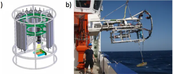
1. As vertical cast: The UVP5 was mounted on the Conductivity, Temperature, Depth (CTD) rosette (Figure 1a). It was deployed vertically from the surface to depths between 100 and more than 5000 m. These profiles were always carried out with the same depth routine: the gear was lowered to 22 m to enable the power-up of the UVP5, was then heaved to the surface again and then the actual profiling started.
Down to 100 m the instrument was lowered with 0.5 m/s speed, below 100 m with 1 m/s. Images were recorded during the whole downcast.
2. As horizontal tow: The UVP5 was mounted on the pelagic in situ system (PELAGIOS; Figure 1b). It was towed at a speed of 1 knot and - recording continuously - lowered to discrete sampling depths between 20 m and 1000 m depth.
At these discrete sampling depths, horizontal tows between 10 and 20 minutes were performed. Because the sampling depths and towed distances differed substantially between the casts, they were not used for the quantitative comparison of eddy and non-eddy stations. One horizontal tow was used to describe the change in certain abundances over time and distance, but not over depth. Data from tows at two stations were used for a comparison of UVP5 and PELAGIOS. Images of Poeobius sp.
that were recorded during horizontal tows were included in the length determinations and for the observation of feeding behaviour (3.2.1 and 2.5.2).
2.1 The Underwater Vision Profiler and PELAGIOS
The Underwater Vision Profiler (Picheral et al. 2010) consists of a black-and-white CCD (charge-coupled device) camera in a pressure-proof case and two red LED light arrays in a defined distance to the camera. During a cast the instrument takes between 6-11 images per second of the illuminated area between the light arrays. The raw images are directly processed within the UVP5 processor unit: particles between 0.006 cm and 2.679 cm size are measured and values are stored in a data file.
Additionally, images of single objects larger than 500 µm are saved as so-called
vignettes. These can be analysed later and sorted for detritus, phyto- and zooplankton categories, first with an automatic sorting system and then validated by manual sorting. The volume recorded by the UVP5 is defined by the known volume of the illuminated field and the frequency of image acquisition. The instrument provides a quantitative method for the estimation of particle and meso- to macrozooplankton concentrations in the water column.
The pelagic in situ observation system (PELAGIOS) is a towed video camera system that was developed under the lead of Dr. Henk-Jan Hoving (GEOMAR). It consists of an HD (high definition) camera and battery packs in pressure proof cases, as well as LED lights that are mounted into an open frame. The field of view of PELAGIOS is unknown, therefore the instrument provides qualitative data. Semi-quantitative comparisons between tows are possible, but no quantitative assessment can be done so far.
Figure 1: a) The Underwater Vision Profiler (UVP5) mounted in a CTD rosette; image modified from Picheral et al. (2010). b) UVP5 mounted onto the towed pelagic in situ observation system PELAGIOS.
2.2 Study area
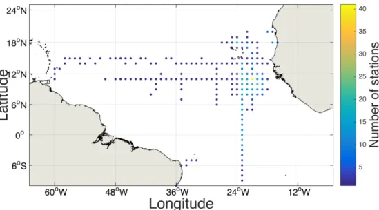
From the 993 profiles considered, most data were available from the eastern tropical North Atlantic between 8 - 12 °N and 19 - 23 °W and from the 23°W transect between 14°N and 5°S. Single cruises covered stations on the Mauritanian and Brazilian shelf, on the 11°N transect between 18°W and 50°W and the 13°N and 14°N transect between 18°W and 58°W as well as the region around the Cape Verde archipelago (Figure 2 and Table 1).
Figure 2: Study area in the tropical Atlantic. Stations are pooled on a 1 degree grid; each dot represents a grid location where UVP5 data were available. The colour of the dots indicates the number of stations at the respective grid location.
Table 1: Overview of the UVP5 profiles and eddies analysed in this thesis. The numbers in brackets indicate the number of horizontal tows; all others are vertical casts.
Cruise Cruise area # UVP5 profiles
Date Eddy type # Profiles in eddy
Eddy Location Eddy recognized on cruise MSM22 5°S - 19°N
20°W - 27°W
109 November 2012
CE ACME ACME AC CE
8 2 2 2 1
18°N 24.5°W 18°N 20°W 13°N 21°W 9°N 23°W 10°N 23°W
no yes no no no MSM23 18°S - 18°N
1°E - 24°W
45 November/
December 2012
CE AC
1 2
14.5°N 23°W 13°N 21°W
no no M096 11°N - 18°N
20°W - 60°W
77 May 2013 AC
AC AC AC CE ACME
1 1 1 1 1 10
14.5°N 42°W 14.5°N 38°W 14.5°N 33°W 14.5°N 31°W 14.5°N 25°W 18°N 25°W
no no no no no yes M097 8°N - 17.5°N
17°W - 24°W
180 June 2013 CE AC CE ACME AC
2 6 2 1 1
11°N 22°W 10°N 21°W 10°N 19.5°W 9°N 21°W 8.5°N 20°W
no no no yes no
ISL00214 17°N 1 February / / / /
25°W 2014 ISL00314 18.5°N - 19
°N 24°W
3 March 2014 ACME 1 19°N 24.3°W yes
M105 7°N - 19°N 17.5°W - 26°W
143 March/April 2014
ACME*
AC CE CE CE
6 2 1 2 1
19°N 25°W 10°N 21°W 10.5°N 19°W 8°N 19°W 11°N 25.5°W
yes no no no no M106 11.5°S - 18°N
21°W-36°W
115 April/May 2014
AC 2 9°N 23°W no
M107 11°N - 20°N 16°W-23°W
73 June 2014 / / / /
PS88b 2°S - 18°N 23°W-24°W
37 November
2014
CE 2 14°N 23°W no
M116 5°N - 18°N 18°W - 58°W
82 May 2015 CE
AC AC CE CE ACME (E1)
1 1 1 1 1 1
11°N 37°W 12°N 35°W 11°N 34°W 11°N 25°W 9°N 23°W 8°N 23°W
no no no no no yes M119 5°S - 18°N
21°W - 24°W
61 (12) September 2015
ACME (E2) AC
3 (1) 1
8°N 23°W 2°N 23°W
yes no MSM49 12°N - 20°N
20°W - 24°W
47 (25) December 2015
CE CE
3 (2) 11 (2)
17.5°N 24°W 16°N 21°W
no yes
Total 993 (37) 36 85 (5)
* the same eddy was sampled during cruise ISL00314, the standing stock/abundance and depth distribution data are merged from these two cruises, while animal sizes are presented separately.
2.3 Environmental data
Environmental conditions, both biotic and abiotic, may impact the distribution of Poeobius sp.. Particle concentration was taken as indicator for biological productivity and as indicator for food availability. Surface particle concentrations were obtained from the UVP5 and calculated as the integrated particle concentration between 20 and 100 m depth. Physical data included temperature, salinity, depth and oxygen concentration and were collected from CTD deployments. Fully calibrated CTD data
were available from all cruises before December 2015. Pre-processed data were used from the cruise MSM49 in December 2015.
CTD and UVP5 data were obtained simultaneously in vertical casts. The only exception for this type of cast was during the cruises ISL00314 and ISL00214, where the UVP5 was deployed as stand-alone instrument and data from the closest (by time and distance) CTD cast at the same station were used. No simultaneous CTD data were available for the transect casts. Environmental conditions of these casts were assessed from the closest CTD profile. The UVP5 has an inbuilt pressure sensor;
therefore CTD data and UVP5 data from the same pressures were related with each other. Environmental data were averaged over the same 5 m depth bins that were used for Poeobius sp. occurrences (see below).
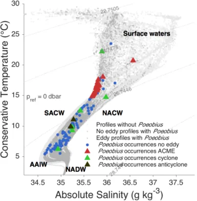
Poeobius sp. distribution is possibly related to water masses, indicated by absolute salinity (SA) and conservative temperature (CT; (IOC 2010). These parameters, and additionally potential density, were computed with version 3.0 of the Gibbs Seawater (GSW) Oceanographic Toolbox that implements the TEOS 10 convention (IOC 2010).
Another physical feature which structures the upper ocean, and which may define the depth distribution of species, is the surface mixed layer. The mixed layer depth was defined as the depth where temperature differed from surface (10 m) conditions by no more than 0.2 °C and density sigma theta by no more than 0.03 as proposed by de Boyer Montegut et al. (2004), and was calculated for all profiles. Poeobius sp.
depths of occurrence were compared with the mixed layer depth for each profile.
Food availability - in case of Poeobius sp. in the form of sinking particles - can limit the distribution of a species. Therefore, particle concentrations at which Poeobius sp.
occurred were determined. These conditions were set into relation with the median particle concentration in non-eddy profiles from vertical casts.
2.4 Assignment of profiles to eddy and shelf
In order to investigate the relation of Poeobius sp. to mesoscale eddies, all profiles were categorized whether inside or outside an eddy. If inside, the type of eddy was determined. It was differentiated between cyclones (CE), anticyclones (AC) and anticyclonic mode-water eddies (ACME). Several mesoscale eddies had already been identified during the respective cruises (the CE on MSM49 and the ACMEs on MSM22, M96, M97, M105, ISL, M116 and M119, see Table 1). Those profiles which were located in these eddies were assigned to the respective eddy category. The eddy status of the undetermined profiles was provided by Dr. Florian Schütte (GEOMAR).
He identified the eddy types by an algorithm that analysed satellite derived sea level
anomaly (SLA) data and evaluated oxygen, temperature and salinity anomalies as described in Schütte et al. (2016b). All profiles that were located within 40 km of an eddy core were assigned to the respective eddy type.
Continental shelves are most commonly defined to have water depths of less than 200 m (Spalding et al. 2007). Only shelf stations from the West African shelf were included here.
2.5 Assessment of Poeobius sp. abundance and depth
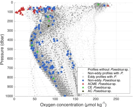
Polychaetes of the genus Poeobius can be identified well on images of the Underwater Vision Profiler (UVP5) as their body plan with its transparent trunk and the (on the black-and-white UVP5 images) dark, spirally gut is very characteristic (Figure 3).
However, identification to species level is not possible.
2.5.1 Image sorting
UVP5 vignettes were processed after the deployment; they were inverted to black- on-white instead of white-on-black, and, among others, the length (equivalent spherical diameter; ESD) and area of the objects are measured. The resulting data file also contained the depth where the image was taken. The classification of the vignettes into detritus, phyto- and zooplankton categories was done with image recognition algorithms (http://www.zooscan.fr; Gorsky et al. 2010) that sort the vignettes into defined categories according to a learning set. Thus predicted profiles were uploaded to Ecotaxa (http://ecotaxa.obs-vlfr.fr/), an online platform that links the classified images into the taxonomic tree. On this platform, the classification was validated, i.e. sorted by hand. The information on assignments was extracted as data files. In this thesis I evaluated data from a total of 1822025 vignettes. I validated the vignette classification of the vertical profiles from cruise MSM49 completely and I checked all profiles from the transect casts of MSM49 and M119 and the vertical casts of M116 and M119 on Poeobius sp. occurrences, which means that I did not validate any other zooplankton categories there. During this check, I often observed wrong assignments of Poeobius sp. into the categories 'Chaetognatha', 'Cnidaria', 'Other_to_check', 'fiber' and 'Eumalostraca'. For all other cruises I only checked those categories.
Information on all profiles was collected in one Matlab database for each cruise. This database contained the complete metadata of each profile (latitude, longitude, time, water depth, sea state, cloud cover, wind), as well as the particle, vignette data and, if
available, CTD data. In the database, concentrations of particles of different size classes and of zooplankton and detritus categories were calculated and stored in a) 5 m depth bins for the vertical casts and
b) 20 second time bins for transect casts.
2.5.2 Size determination
The UVP5 data processing provides size measurements of all particles recorded:
equivalent spherical diameter (ESD, mm) and equivalent spherical volume (ESV, mm3) are determined from the minor and major axis of the best fitting ellipse (Picheral et al. 2010). More than 10% of the Poeobius sp. either had food particles attached or were in an angle unfavourable for length determination, so that the automatic measurements were imprecise. Therefore, additional manual length measurements of all Poeobius sp. were conducted in ImageJ (http://www.imagej.net) with the linear measuring tool. The length was determined by measuring from the base of the tentacle crown to the posterior end (Figure 3). The quality of the measurements was indicated by assigning quality flags, described in Table 1. Only lengths with quality flag 0 were used in this thesis, although a trend of larger animals being bent more often was observed.
Table 2: Description of quality levels in Poeobius sp. measurements.
Quality flag Meaning Description
0 good measurement Poeobius sp. straight and completely on image
1 low accuracy Poeobius sp. bent or partly not on the image
2 no measurement possible Poeobius sp. only in parts on the image
Figure 3: Length determination of Poeobius sp., performed in ImageJ. Poeobius sp. size was measured from the base of the tentacle crown to the posterior end.
To determine the influence of Poeobius sp. on particle flux, its feeding behaviour was investigated. Different feeding stages were described, based on the tentacle position
and attached particles. The percentage of feeding animals calculated for eddies with more than 5 individuals, non-eddy observations and all observations.
Poeobius sp. could not only be observed on the UVP5 images, but also in PELAGIOS videos. In some of these videos, it was possible to see deployed mucus nets of Poeobius sp. In order to detect the potential influence of Poeobius sp. flux feeding on particle flux, the size of the mucus net structures was estimated from the measurement of 5 PELAGIOS video frame shots (provided by H.J. Hoving, GEOMAR) taken on MSM49. As objects on the PELAGIOS images are not scaled, the length of Poeobius sp. was taken as scale for further measurements in ImageJ. The area of the mucus structure was determined by measuring with the polygon tool around the edges of the net (0).
Biomass as a factor accounts for different animal sizes and may represent the impact of a species on the environment better than abundance. Therefore, Poeobius sp.
individual biomass was calculated from the animal's area. The area was estimated as ellipse from body length and width. A common length-width ratio was calculated from the images of 12 individuals. Biomass (µg DW) was determined from this area, using the coefficients by Lehette et al. (2009) for gelatinous zooplankton (specifically siphonophores):
!"= 43.17∗!"#!!.!" ( 1 )
Vertical biomass profiles for two eddies were then calculated from the mean length of the Poeobius sp. in the respective feature and the corresponding width from the above described length/width relationship. Biomass per individual was multiplied with the abundance per depth bin.
2.5.3 Calculations and binning
Abundances and standing stock
Pseudo-replication by having multiple profiles in one location was avoided by pooling:
a) all profiles within 0.01° and sampled within less than 30 days
b) all profiles within the same eddy and sampled within less than 30 days.
All standing stocks presented here were averaged for all profiles of one station. The standing stocks and depths of Poeobius sp. in the eddies on M105 and ISL00314 were averaged because it was the same feature on both cruises.
In order to compare profiles with different maximum depths, i.e. different scanned volumes, the following approach was used to calculate standing stocks: Only data from profiles that reached depths of more than 550 m were included in the analysis.
Then, all vertical profiles were cut off at 600 m for being able to compare eddy and non-eddy stations as some of the eddy profiles did not exceed this depth. Poeobius sp.
abundance (ind m-3) was determined by dividing the count by the profile volume (Vtp). Standing stocks were calculated by multiplying the abundance with the maximum depth of the profile (pmax).
Standing stock= !"#$%
!!" ∗ p!"# ( 2 )
For presenting the horizontal distribution of Poeobius sp., the mean standing stocks found at stations were binned on a 1-degree grid.
Horizontal tows
Horizontal tows provide information of particle and zooplankton abundances at discrete sampling depths. They enable a comparison of these abundances over time and distance without depth changes. This was used to investigate the effect of high abundances of Poeobius sp. on the particle concentration in the ACME on M119. The discrete sampling depths were identified as those measurements that differed by less than 3 dbar between 20 s time bins. Particle abundance (0.8 - 5 mm), Poeobius sp.
abundance and the abundance of large aggregates (> 600 µm) identified from the UVP5 images were plotted over distance at 50 m and 100 m depth. Distance was calculated from time, assuming 1 knot towing speed.
Other zooplankton
An assessment of Poeobius sp. abundance in relation to other zooplankton in the M116 (E1), M119 (E2) ACMEs and some background profiles was done. Background data included validated profiles of the cruises MSM22, MSM23 and M106. Seven categories of zooplankton were differentiated: copepods (integrating everything copepod-like), phaeodaria, collodaria, other rhizarians, 'other' (containing all other identified zooplankton groups, e.g. crustaceans, medusae etc.) and 'to check' (containing all unidentified zooplankton). Integrated abundances of all these categories and of Poeobius sp. were plotted as stacked barchart. The percentage of each category within the whole zooplankton was calculated and again illustrated in a stacked barchart.
2.6 Assessment of particle concentrations, sizes and flux
The flux-feeder Poeobius sp. may have an impact on particle concentrations and sizes and resulting flux when it is abundant. Highest polychaete abundances were found in the ACMEs sampled on cruises M116 and M119, which were both detected at 8°N and 23°W. Data from 8 other cruises were available at this location and used as background information. Particle concentrations (0 to 600 m depth) on the 23°W section were plotted between 7°N and 12°N. Particle density anomaly was derived by interpolating background and eddy data on a 0.5 degree grid using the Matlab function interp2 with the linear interpolation method and subtracting the gained background density from the eddy densities.
The abundance and integrated volume of particles in different size classes was plotted against size (abundance-size spectrum and volume-size spectrum) as described by Iversen (2010). Depths of particle removal were identified by calculating eddy particle data and median background particle data (profiles within one degree of the eddy profiles position) integrated for three depth layers: 1. The surface: from 12.5 m to the depth, below which the first Poeobius sp. occurred, thereby covering the mixed layer. 2. The Poeobius sp. layer: between the shallowest and the deepest Poeobius sp. occurrence. 3. The layer below the deepest Poeobius sp.
occurrence: a layer of the same thickness as each of the first two.
Particle fluxes were calculated from the abundance and sizes of particles in single size classes using the coefficients from Tables 1 and 2 of Kriest et al. (2002). The relation of particle diameter to particle mass was taken from Table 1. Mass in nmol N was converted to mmol C by using the Redfield ratio (Redfield et al. 1963), the relation of diameter to sinking speed was taken from Table 2, assuming a sinking velocity of 2.8 m d-1 for a particle of 0.002 cm size (Kriest 2002). Coefficients from Alldredge et al. (1998) were used to calculate carbon content from mass:
!!"#!$%= c!"#!$%∗ DSE!"#$!"#!$% ( 3 )
!"#!!!""!= !!!""!∗!"!!"!!!""! ( 4 )
With: minsitu = molar mass (mmol C), cinsitu = 273, zetainsitu = 1.62, sinkk2002 = sinking velocity (m d-1), bk2002 = 132, DSE = size (cm), and etak2002 = 0.62.
For each size class, the flux (F, mg C m-2 d-1) by a single particle was calculated from the particles sinking velocity (sinkk2002) and its mass (min situ). By multiplying with the atomic mass of carbon (12 g mol-1), mmol C was converted to mg C.
! = !"#$_!2002∗!_!"#!$%∗1000∗12 ( 5 )
Individual particle masses and fluxes of each size class were multiplied with the particle abundance in the respective 5 m depth bin. Particle mass and flux were
integrated over size classes between 140 µm and 2.66 mm in order to obtain the total mass flux in this size range. Smaller particles were excluded in the flux calculation because these are not quantitatively measured with the UVP5. Particles larger than 2.66 mm were not used in order to avoid the inclusion of Poeobius sp. in the measurements.
2.7 Calculation of Poeobius sp. respiration and carbon utilisation
Respiration and carbon utilisation rates were calculated for E1 and E2 in order to relate changes in particle flux to Poeobius sp. abundance. Thuesen and Childress (1993) reported respiration rates of 0.068 µmol g-1 h-1 for Poeobius meseres. This value was taken as baseline for the following calculations. Thuesen and Childress (1993) detected no allometric relation so this was omitted here as well. The authors measured respiration at 5°C. Poeobius sp. was found at higher temperatures of around 15°C in E1 and E2, therefore a Q10 value of 2 (Moloney and Field 1989) was applied, resulting in a doubling of the respiration rate. Multiplication with 24 resulted in the respiration rate per day. Taking into account that Poeobius sp. is a gelatinous organism and thus consists to more than 95% of water, body weight (ww_poeo) was calculated from the body volume as the weight that the same volume of seawater (with a density of 1.023 g ml-1) would have. Body volume (vol_poeo) was calculated assuming a body shape of a prolate ellipsoid. The mean length (length_poeo) of the animals in E1 and E2 was calculated from the measurements described in 2.5.2 and body width estimated from the mean length and the length/width ratio (lwr) as described in the same paragraph.
!"!!"#"= 4∗!! ∗ !!∗!"#$%!!"#"
!"# ∗ !!∗!"#$%ℎ!"#" ( 6 )
!!!"#"= !"!!"#"∗1.023 ( 7 )
With this body weight, respiration rates per individual and - by multiplying with the abundance in the single depth bins of E1 and E2 - per cubic metre were determined.
Integrated community respiration per square metre was obtained by adding up the respiration rates determined for the single depth bins. The respiration rates (R_poeo, in µl O2 d-1) were converted into carbon utilisation rates as described by Steinberg et al. (1997):
!!"#$= !!"#"∗ !"
!!.! ∗0.97 ( 8 )
where 12/22.4 is the weight of C in 1 mol (22.4 L) of CO2 and 0.97 is the respiratory quotient, i.e. the relative amount of CO2 produced from O2 taken up by the animal.
2.8 Comparison of UVP5 and PELAGIOS counts
The volume recorded by the UVP5 is comparatively small and it also takes images only every few centimetres and possibly misses rare animals. Thus, for assessing the applicability of using the UVP5 for distribution analysis of a rare species, such as Poeobius sp., UVP5 counts from horizontal tows were compared with video counts from the pelagic in situ observation system (PELAGIOS) that were obtained in parallel. Counts of Poeobius sp. in PELAGIOS transects for each discrete sampling depth were kindly provided by Henk-Jan Hoving. Poeobius sp. counts from UVP5 data were obtained by multiplying the abundance (ind m-3) at each discrete sampling depth (determined as described in 2.5.3) with the respective volume. Four deployments (each two eddy and eddy reference casts) from cruise MSM49 were compared. A linear regression between the counts of the two instruments was tested.
An approximation of the volume recorded by PELAGIOS was calculated from the relationship between the counts.
2.9 Statistics
2.9.1 Comparisons between eddy and non-eddy stations
Most bins and even most profiles had only 0 or 1 observations, which made the statistical comparison of abundances difficult. In order to compare bin data of Poeobius sp. in vertical profiles with environmental conditions only presence/absence data were used. In the horizontal tows, the scanned volume per bin on the single transects was assumed to be comparable as towing speed did not differ. Also the bins were larger than in the vertical casts (20 s bins instead of 5 m (equaling 5 s) bins, i.e. fourfold volume), therefore, abundances (ind m-3) were calculated and used in the analysis.
All statistical tests were done in the R statistical environment (R Development Core Team, 2011). Because sample sizes were very different and data not normally distributed (tested with the Shapiro-Wilk test (R-function shapiro.test, stats package)), the following non-parametric statistical tests were applied:
1. The two sample Wilcoxon rank test (also called Mann-Whitney U-test, R-function wilcox.test, stats package) was used for comparing means of, for example, Poeobius sp.
abundance between stations and between different eddy types.
2. The Kolomogorov-Smirnov test (R-function ks.test, stats package) was used for comparing the distribution of data points (e.g. depth occurrences) between different eddy types.
The abundance-size and volume-size spectra of particles in E1 and E2 were compared to the background spectra by an ANCOVA (R-funtion aov, stats package).
Two depth layers were compared from each environment. First, the linear regression of the log-log transformed data of the respective layers was calculated and tested for significance. Size was used as independent variable, abundance and volume, respectively, as response variable. The layer description was used as categorical factor. Then the interaction of the categorical factor with the independent variable was determined by applying an ANCOVA to one model with and one model without the interaction of the factors. The two models were compared by an ANOVA (R-function anova, stats package) and this significance level taken to describe difference in slope. If the interaction was not significant, the model without interaction was concluded to be the most parsimonous model and the significance of the categorical factor determined therein was taken as description of the difference in intercepts. Because the results for the abundance-size and the volume-size ANCOVA were the same, they were summarised in one table for E1 and E2 each.
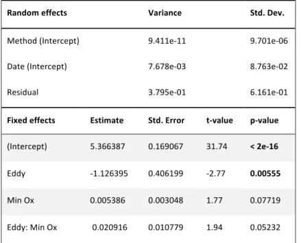
2.9.2 Generalized linear mixed model
In order to include multiple potential factors, which could influence Poeobius sp.
depth distribution, a generalized linear mixed model (GLMM) was fitted by maximum likelihood (Laplace Approximation), as proposed by Bolker et al. (2009) for this type of data. The mean depth of occurrence of each profile with Poeobius sp.
presence was modelled with the R-function glmer (R-package lme4) with Gamma error distribution and link = log to account for overdispersion. Sampling method and time were set as random effects. Fixed effects included environmental data from the respective profiles (latitude, longitude, month, surface particle concentration of large, medium and small particles, minimum oxygen concentration). Due to overdispersion, p-values for Wald's t (Bolker et al. 2009) were analysed to evaluate the most important factors for Poeobius sp. mean depth. Model selection for further identification of important effects was done by stepwise regression (ANOVA): In every step the least significant fixed effect was removed from the model. The Chi2 and p-value for Chi2 from an ANOVA of the model with and without the fixed effect were calculated and the Akaike Information Criterion (AIC) compared between the two model versions. A factor was excluded if this lowered the AIC of the model.
3 Results
A database of 993 UVP5 profiles and the corresponding environmental data from large parts of the tropical Atlantic were analysed for Poeobius sp. occurrence and horizontal and vertical distribution. Poeobius sp. abundance in different types of eddies and its relation to particle abundance, sizes and resulting flux were calculated. The 993 profiles were taken at 719 stations. A total of 36 stations were identified to be located inside a mesoscale eddy.
3.1 Poeobius sp. distribution and eddy association in the tropical Atlantic
Poeobius sp. abundance and distribution was evaluated from non-eddy and eddy stations. The resulting horizontal distribution across the tropical Atlantic and the vertical distribution in the water column are shown in the following chapter. Also, Poeobius sp. distribution in relation to water masses (i.e. the physical environment) are described and the characteristics of the Atlantic Poeobius sp. are pointed out.
3.1.1 Horizontal distribution
A total number of 481 Poeobius sp. was found in a database of 993 UVP5 profiles in the tropical Atlantic between 16°W to 46° W and 5°S to 20°N. While 197 observations came from non-eddy stations, 284 were observed at eddy stations.
Non-eddy stations
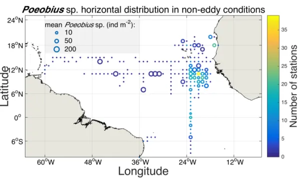
Poeobius sp. was found at 108 non-eddy stations with vertical casts in the tropical Atlantic. Locations of occurrence ranged between latitudes of 5°S and 20°N and between longitudes of 16°W and 46°W (Figure 4). In the vertical casts, Poeobius sp.
was observed at roughly every tenth station, numbers ranged between 0 and 3 polychaetes per cast. This resulted in standing stocks of 0 - 123 ind m-2 at the grid points and a mean standing stock of about 10 ind m-2 in the area covered by vertical casts. Highest standing stocks were observed at 11°N between 31°W and 33°W.
However, Most individuals, in the eastern tropical North Atlantic between 8°N - 13°N and 19°W - 23°W, Poeobius sp. was observed most frequently. There the sampling coverage was highest. Otherwise Poeobius sp. showed no clear distribution pattern in the tropical Atlantic Ocean.
Figure 4: Horizontal distribution map of Poeobius sp. at non-eddy stations in the tropical Atlantic Ocean; averaged on a 1 degree grid from vertical UVP5 casts. Dots indicate grid locations where UVP5 data were available, open circles indicate the occurrence of Poeobius sp.
at this location. The size of the circle represents the mean standing stock (ind m-2) of Poeobius sp. at the respective grid point and the colour the number of stations. Only data from the upper 600 m are included.
Eddy stations
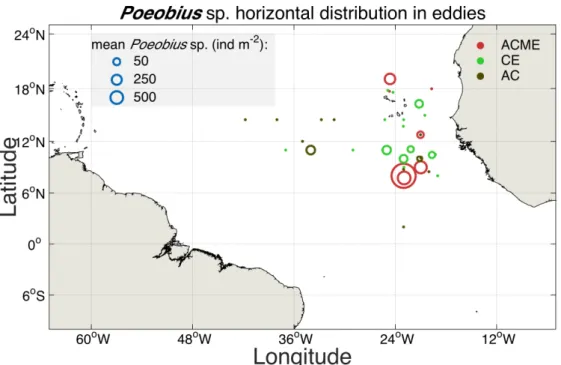
Poeobius sp. was observed at 17 out of 36 eddies that were sampled between 2°S and 19°N and 19°W and 41°. Of these eddies, 17 were classified as cyclones (CEs), 13 as anticyclones (ACs) and 6 as anticyclonic modewater eddies (ACME, Figure 5). In CEs and ACs, numbers ranged between 0 and 1 individuals per cast resulting in standing stocks of 0 to 110 ind m-2 and a mean standing stock of 30 ind m-2 and 10 ind m-2, respectively. In ACMEs, Poeobius sp. had numbers between 0 and 64 per cast and standing stocks between 0 and 6470 ind m-2 with a mean of 1280 ind m-2.
Figure 5: Horizontal distribution map of Poeobius sp. in eddies in the tropical Atlantic Ocean from vertical UVP5 casts. Dots indicate eddy locations where UVP5 data were available, open circles indicate the finding of Poeobius sp. in that eddy. The size of the circle represents the mean standing stock of Poeobius sp. in the respective eddy and the colour the type of eddy.
ACME stands for anticyclonic modewater eddy, CE for cyclonic eddy and AC for normal anticyclones. Only data from the upper 600 m are included.
Shelf conditions
Most eddies in the eastern tropical North Atlantic form on the West African shelf and propagate westward from there. Increased abundances of a species such as Poeobius sp. at shelf stations compared to open ocean stations would indicate eddy transport.
Only 26 out of 993 UVP5 profiles were located on the West African shelf. No Poeobius sp. was found at any of these shelf stations.
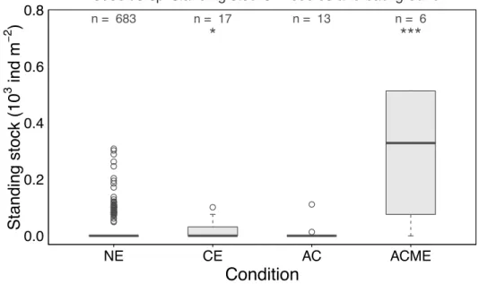
Comparison between Poeobius sp. standing stocks at non-eddy and eddy stations
A significantly (Mann-Whitney U: p<0.001) larger standing stock was found at ACME stations (mean of 1285 ind m-2) compared to non-eddy stations (mean of 11 ind m-2) in vertical casts. The standing stock was about 100fold larger at these stations. Median standing stock size was 0 ind m-2 at non-eddy stations and 330 ind m-2 at ACME stations (Figure 6). Mean standing stocks at non-eddy stations and in CEs (mean of 18 ind m-2) differed significantly (Mann-Whitney U: p<0.05), but the median was 0 in both conditions. There was no difference in abundances between vertical non-eddy casts and anticyclonic eddies (Mann-Whitney U: p > 0.05). The largest standing stock was found in the M116 ACME with 6470 ind m-2.