Strong time dependence of ocean acidi fi cation
mitigation by atmospheric carbon dioxide removal
M. Hofmann 1*, S. Mathesius 2*, E. Kriegler1, D.P. van Vuuren 3,4 & H.J. Schellnhuber1
In Paris in 2015, the global community agreed to limit global warming to well below 2C, aiming at even 1.5C. It is still uncertain whether these targets are sufficient to preserve marine ecosystems and prevent a severe alteration of marine biogeochemical cycles. Here, we show that stringent mitigation strategies consistent with the 1.5C scenario could, indeed, provoke a critical difference for the ocean’s carbon cycle and calcium carbonate saturation states. Favorable conditions for calcifying organisms like tropical corals and polar pteropods, both of major importance for large ecosystems, can only be maintained if CO2emissions fall rapidly between 2025 and 2050, potentially requiring an early deployment of CO2removal techniques in addition to drastic emissions reduction. Furthermore, this outcome can only be achieved if the terrestrial biosphere remains a carbon sink during the entire 21st century.
https://doi.org/10.1038/s41467-019-13586-4 OPEN
1Potsdam Institute for Climate Impact Research, Potsdam, Germany.2GEOMAR Helmholtz Centre for Ocean Research Kiel, Kiel, Germany.3Copernicus Institute for Sustainable Development, University Utrecht, Utrecht, Netherlands.4PBL Netherlands Environmental Assessment Agency, The Hague, Netherlands. *email:hofmann@pik-potsdam.de;smathesius@geomar.de
1234567890():,;
U
nrestrained anthropogenic carbon dioxide (CO2) emis- sions would not only cause global mean surface tem- peratures to exceed the Holocene range1but also modify the ocean chemistry in an unprecedented way2. The Paris Agreement, struck at the 21st Conference of the Parties (COP21) in Paris in 2015, intends to limit global warming to 1.5–2C. This multilateral consensus is based on the assessment that highly disruptive environmental impacts could be expected if these targets are exceeded3–5. Research shows that reaching the 2C goal with reasonable probability already requires ambitious mitigation efforts worldwide6. However, while the 2C target is assumed to be sufficient to prevent reaching most of the climate system’s tipping points3,5, it might not be enough to keep the oceans biogeochemistry and ecosystems intact7,8.This is of particular concern, because once the ocean is severely altered by warming and acidification, it would take many cen- turies to bring it back to the preindustrial state7, even long after the atmospheric CO2 concentration has returned to its pre- industrial level. This slow response of the ocean to atmospheric changes is in part related to the long time scale of the overturning circulation, where water masses can be out of contact with the atmosphere for more than 1000 years before they are completely circulated back to the surface and re-establish an equilibrium with atmospheric CO2concentrations and temperatures.
Approximately 26% of current anthropogenic CO2 emissions have been absorbed by the oceans already9, which has reduced the oceanspH value from 8.21 to 8.10 (ref.1). This trend is a serious threat to many marine organisms, especially calcifying species that require seawater with an aragonite saturation state larger than one (Ωa >1) to build shells and skeletons. Among the most important calcifiers are tropical reef-building corals and pter- opods, planktonic snails dwelling in the pelagic zone. Both are known to be threatened by global warming and ocean acidifica- tion10–13. Coral reefs are among the most important ecosystems because they provide habitat to more than a million species and ecosystem services to more than hundreds of millions of people14. As a result of marine heatwaves, overfishing, pollution, storms and unsustainable coastal development, the distribution and abundance of tropical corals has been reduced by approximately 50% over the past 30 years5. Marine heatwaves lead to coral bleaching and become more frequent with global warming.
Numerous studies have shown that even a limitation of global warming to 2C compared to preindustrial conditions will put almost all tropical coral reefs at risk11,12,15. Ocean acidification puts additional pressure on corals because it reduces the satura- tion state of aragonite, with the result that corals have to spend more energy on calcification, grow slower, get more vulnerable to diseases and become less competitive5,16. The weakening of coral reef resilience can have the consequence that macroalgae over- grow the corals to the extent that the whole reef shifts to an algal- dominated regime10with reduced biodiversity. The other calci- fiers addressed here, pteropods, are small planktonic molluscs that produce thin aragonite shells and therefore require an environment that is oversaturated with respect to aragonite (Ωa >1)17. They are highly abundant in temperate and polar waters5and play a crucial role in the marine food web13, because they provide a link between phytoplankton and fish, birds and whales5. The reduction in the aragonite saturation state Ωa already affects the ability of pteropods to produce shells, swim and survive5,18. Especially at high latitudes, where ocean acid- ification is most severe, large regions are expected to become uninhabitable for pteropods, as we show below.
Advocates of planetary-scale interventions have argued that artificial carbon dioxide removal (CDR) from the atmosphere might solve both global warming and acidification problems.
However, it has been shown7 that even extreme CDR
interventions would fail to restore marine chemistry within many centuries, if they are deployed too late, i.e., after the ocean has already been severely altered7,19,20. This insight is critical for the scientific assessment of the purported benefits of geoengineering measures21–25. It has been maintained23,26 that planetary-scale technical remedies offer an ultimate chance of saving the global environment once mitigation policies become insufficient and that CDR can be an effective response because it reduces both climate and acidification risks26. However, CDR can only be effective if deployed early and combined with massive mitigation strategies, which has been found in several studies on 2C pathways that combine stringent mitigation strategies and CDR27–29. The amount of CO2 that can be removed from the atmosphere by CDR options is limited by land availability, sto- rage capacity, water requirements or energy consumption30, thus cannot be expected to counteract unmitigated emissions.
Here, we show that deep mitigation pathways, such as Shared Socioeconomic Pathway 1 (SSP1)-2.6, may also limit ocean acidification when embedded into aggressive climate-action scenarios28,29. This study aims to demonstrate the importance of correct timing for CDR deployments as an accompanying measure for existing and ambitious CO2 emission reduction pathways to maintain global warming within the safe range and efficiently protect the marine environment. More specific, we investigate whether the limited and timely application of atmo- spheric CDR could help to maintain global warming in the range between 1.5 and 2C and simultaneously prevent calcifying organisms, such as tropical coral reefs and pteropods, from ser- ious damages. In previous studies by Vaughan et al.24, Frölicher and Joos20and Mathesius et al.7, the importance of the timing of mitigation and CDR measures, with respect to the irreversibility of ocean acidification and their potential impacts on marine biota, was already highlighted. Based on thefindings of these previous studies, our work tries to answer the following questions:
Given that society would decide on the deployment of atmo- spheric CDR starting as early as possible (i.e., during the mid 2020s), would it matter if we postponed this deployment by 50 years under the constraint of removing exactly the same amount of CO2 as in a case with earlier action? Would the benefits of delayed CDR measures be comparable to those of early CDR deployment? The outcome of our research suggests that only an early deployment of CDR would have the potential to mitigate damages on marine ecosystems due to ocean acidification, pro- jected to occur even under the low emission SSP1-2.6 scenario, by concomitantly limiting global warming to 1.5C. In this context, CDR only makes sense if rapid decarbonization of the world economy succeeds—not if it founders.
Results
Model experiments and strategy. We employed the model CLIMBER-3α + C (see Methods), an Earth system model of intermediate complexity (EMIC) based on the abiotic version of CLIMBER-3α31, to simulate the following CO2 emissions sce- narios from 1800 to 2200:
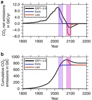
The baseline scenario SSP1-2.6 (ref.27) was designed to meet the 2C climate target. Since the original SSP1-2.6 scenario ends already in 2100, we have extended it until 2200 by linearly reducing the net negative emissions to zero from 2100 to 2150 (see black line in Fig.1). Compared to the baseline, ourfirst newly designed CDR scenario assumes an additional removal of atmospheric CO2 of in total 109 Gigatons of carbon (GtC) by CDR measures between 2025 and 2050. In 2050, the net emissions reach zero (see blue line in Fig. 1). In a subsequent consolidation phase, CDR guarantees net zero emissions until 2050–2075, by an additional extraction of 64 GtC. In contrast to
SSP1-2.6, this modified scenario ignores negative emissions between 2075 and 2200. Henceforth, we refer to this scenario, which extracts a total of 63 GtC more than SSP1-2.6 over the entire CDR period (between 2025 and 2150), as“EARLY”.
The second modification to the baseline scenario was motivated by the question of whether it would make a large difference in the resulting climate and marine ecosystem response if we postpone the CDR interventions suggested by EARLY by 50 years. Here, we initialize the CDR deployment again by removing an extra 109 GtC total between 2075 and 2100 (see red line in Fig.1) by subsequently decreasing the negative CO2 emissions between 2100 and 2150 to zero, such that the cumulative reduction in comparison to SSP1-2.6 amounts to exactly 63 GtC (equal to the total extra reduction assumed in EARLY). Henceforth, because the CDR starts 50 years later, we refer to this scenario as“LATE”.
In contrast to a similar study by Frölicher and Joos20, who demonstrated what would have happened if society had stopped anthropogenic emissions in 2000 in comparison to a weak and strong mitigation scenario until 2100, our work tries tofind realistic timing for CDR interventions that are not only eligible to meet the 1.5C target but also to protect marine biota.
CLIMBER-3α+C includes an isogeochemical (i.e., it does not account for river-runoff and sedimentation loss) marine carbon cycle model coupled with an NPZD (nutrient, phytoplankton, zooplankton and detritus) biogeochemical model but does not include a state of the art terrestrial carbon cycle and land biosphere model. To emulate the impacts of the terrestrial biosphere on the global carbon cycle, which is an important component of the climate system32, CLIMBER-3α+C was coupled with a box model similar to a reduced version of the terrestrial model by Wigley33 (see Methods). The three terrestrial boxes accounting for the carbon budgets of living plants, detritus and soil were interactively coupled to the CLIMBER-3α+C atmospheric module. The effects of land use change were not accounted for because the emission scenarios already included them.
The terrestrial box model mainly parameterizes the gross primary production rate (GP) of living plants, respiration rate (R) and remineralization and oxidation rates of detritus and soil (Q10 values). The model sustains a net carbon sink over the entire simulation period34.
To achieve a quasi-steady state representing the unperturbed preindustrial climate, a spin-up of CLIMBER-3α+ C of more than 6000 years was performed. The control model simulation arrives at a climate state comparable to that of the observational data1, with an atmospheric CO2 concentration of 284.0 ppmv, and a globally averaged annual mean sea surface pH value of ~8.13.
We performed thefirst scenario analyses by running the EMIC from 1800 until 2005 with historical CO2 emission data35. Subsequently, the model was forced with CO2emissions by the SSP1-2.6, EARLY, and LATE protocols until the year 220029.
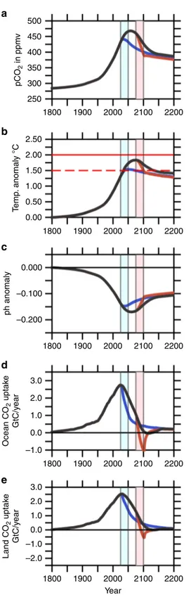
Emission scenarios. In agreement with previous studies35,36 forced by SSP1-2.6 emissions, atmospheric levels of CO2 are projected to increase to ~470 ppmv (Fig. 2a), while the global mean temperature peak around year 2075 is expected to be
~1.8C above preindustrial values (Fig. 2b) for the SSP1- 2.6 simulation. Accordingly, the globally averaged sea surface pH values for the oceans display a pronounced decrease during the middle of the 21st century, exceeding values of −0.17 units (Fig. 2c) for the SSP1-2.6 simulation. Compared to the SSP1- 2.6 scenarios over the entire simulation, the scenario EARLY leads to much lower atmospheric CO2levels, with a maximum of about 440 ppm, resulting in global warming of nearly 1.5C and a maximum decrease in pH of approximately 0.15 units, with consecutively decreasing anomalies after the year 2050 (see Fig.2a–c). The EARLY scenario can be compared with other very low emissions scenarios falling below SSP1-2.6 in the literature.
Rockström et al.37proposed a scenario of halving CO2emissions every 10 years from 2020 onwards that uses CDR only to a very limited extend to reach net zero CO2emissions by mid century.
The lowest SSP scenarios limiting radiative forcing to 1.9 Wm2 by the end of the century, including an SSP1-1.9 scenario (see Fig.3) by the IMAGE model, also reach net zero CO2emissions by mid century38. These and similar scenarios were assessed by the recent IPCC Special Report on 1.5C (Chapter 2, Rogelj et al., SR1.5)5, which found that on average about two thirds of the faster phase out of CO2 emissions compared to associated 2C scenarios were due to stronger emissions abatement and only one third due to earlier deployment of CDR. Hence, the acceleration of CO2phase out compared to SSP1-2.6 does not need to come all from additional CDR as assumed in the EARLY scenario.
Obviously, the LATE-scenario is not suited to mitigate climate change efficiently in any case, which notably occurs during the critical time interval between 2025 and 2100.
CO2 uptake by land and oceans. Continuously rising CO2 emissions have led to elevated atmospheric CO2 levels, which generated a fertilization effect for the land biosphere (Fig.2e)
33,34 and increased atmosphere-ocean gradients of the partial pressure of CO2, resulting in a net CO2 flux into the oceans (Fig. 2d)39. The average air-to-sea CO2flux between 1990 and 1999 simulated by SSP1-2.6 amounts to 1.99 GtC per year, while the land biosphere amounts to ~1.85 GtC per year. The numbers agree well with the values given by the Fifth Assess- ment Report (AR5) of the IPCC1whereby oceans and land take 1.7 ± 0.5 and 1.4 ± 0.7 GtC per year during this period of time, respectively. These numbers increase remarkably until 2017 to 2.60 GtC per year for the ocean and 1.54 GtC per year for land in case of SSP1-2.6. During the late twenties in the 21st century, the oceanic uptake of CO2is projected to reach its maximum at 2.75 GtC per year by SSP1-2.6 (see Fig. 2d) and land will take up a maximum of 2.75 GtC in year 2025. Compared to all other emissions scenarios discussed here, EARLY reveals the lowest cumulative oceanic uptake of atmospheric CO2 between 2025 a 12.0
b
SSP1–2.6 Early Late
SSP1–2.6 Early Late
8.0 4.0 0.0 –4.0 –8.0
1000 800 600 400 200 0
1800 CO2 net emissions in GtC/yr
Cumulative CO2 emissions in GtC
1900 2000 Year
2100 2200
1800 1900 2000 Year
2100 2200
Fig. 1 Emission scenarios utilized in this study.Time line of the three anthropogenic CO2emission scenarios between 1800 and 2200.aCO2net emissions in GtC year1.bCumulative CO2emissions in GtC.
and 2075, leading to a decrease in global mean sea surface pH of 0.15 units (see Fig.2c,d).
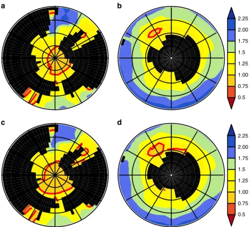
Aragonite saturation in polar waters. In line with thefindings by Hauri et al.40, even in the highly mitigated scenarios (SSP11-2.6), we found a development of a seasonal carbonate undersaturation with respect to aragonite at sea surface. In this regards, our model simulations clearly show the advantage of an early CDR deploy- ment (EARLY) against the LATE-scenario where the action is deferred by 50 years. Figures4and5show the seasonal mean value of the sea surface aragonite saturation stateΩain the Arctic and the Antarctic during the seventies of the 21st century for January until March, and July until September, respectively. In case of EARLY, the maximum area of surface waters during winter season which is undersaturated with respect to aragonite (Ωa<1) in the Arctic and the Southern Ocean remains below ~5,929,000 km2. For LATE, the winter season area with aragonite undersaturated seawater expan- ded over the Laptev and Beaufort Seas and most of the Weddell Gyre covers a total of 10,626,000 km2, which is nearly twice the area of the undersaturated water masses in EARLY.
Coral reef calcification rates. To assess the dependence of gross community calcification in stony corals on sea surface tempera- ture (T) and the aragonite saturation state (Ωa), we use the empirical rate law by Silverman et al.41which has been derived by utilizing data of >9000 reef locations. Given thatGi(see Methods) is the rate of inorganic aragonite precipitation, the gross com- munity calcification rate depends onT andΩa as follows:
TGgrossGiexp k0p ðTToptÞ Ω2a
2!
;
wherek0p=1C 1and Topt represents the optimal temperature for calcification found between 27 and 28C41.
Here, we apply the relation given above to assess the potential impacts of the three scenarios investigated in our study on the gross community calcification rates of tropical coral reefs during the fourties and the seventies of the 21st century, where the sea surface pH decline is at maximum, by utilizing the summer solstice temperatures (June/December for the northern/southern hemisphere). for Topt. Therefore we calculated the change in TGgross during these two time intervals relative to their preindustrial values at the more than 10,000 locations in the tropical coral reefs provided by the Reef Base (M. Tupper et al., ReefBase: A Global Information System on Coral Reefs, http://
www.reefbase.org). In all scenarios investigated in our study, tropical coral reefs are affected by the impact of anthropogenic CO2emissions. The largest impacts are projected to occur in the Indonesian archipelago, where the mixed layer depths are relatively shallow, leading to a higher accumulation of
12.0 8.0
SSP1–2.6 Early Late SSP1–1.9
4.0 0.0 –4.0 CO2 net emissions in GtC/yr
–8.0
1800 1900 2000
Year
2100 2200
Fig. 3 Utilized emission scenarios in comparison to SSP1-1.9.Time line of the three anthropogenic CO2emission scenarios in comparison with the SSP1-1.9 scenario38between 1800 and 2200 in units of GtC year1. 500
b a
c
d
e pCO2 in ppmv
450 400 350 300 250
2.50
Temp. anomaly °Cph anomalyOcean CO2 uptake GtC/year 2.00 1.50 1.00 0.50 0.00
0.000
–0.100
–0.200
1800 1900 2000
Year
2100 2200
1800 1900 2000 2100 2200
1800
3.0 2.0 1.0 0.0 –1.0
3.0
Land CO2 uptake GtC/year 2.0 1.0 0.0 –1.0 –2.0
1900 2000 2100 2200
1800 1900 2000 2100 2200
1800 1900 2000 2100 2200
Fig. 2 Evolution of important climatological variables.Time evolution of atmospheric and global mean sea surface values of climatologically relevant parameters during the entire model simulation between years 1800 and 2200.aatmospheric pCO2concentrations in ppmv;bglobally averaged and annual mean atmospheric temperature anomaly at the Earth surface inC;csea surface pH anomaly;duptake of CO2by the ocean in GtC year1;euptake of CO2by the land biosphere in GtC year1. The light blue and the pink stripe mark the period of the initial carbon dioxide removal (CDR) measures for the EARLY and LATE scenarios, respectively.
2.25 2.00 1.75 1.5 1.25 1.00 0.75 0.5
2.25 2.00 1.75 1.5 1.25 1.00 0.75 0.5
a b
c d
Fig. 4 Polar aragonite saturation during boreal winter season.Decadal mean (2070–2080) aragonite saturation stateΩaduring January–March for EARLYaArctic andbAntarctic and LATEcArctic anddAntarctic. TheΩa=1 iso-line is drawn in red.
2.25
a b
c d
2.00 1.75 1.5 1.25 1.00 0.75 0.5
2.25 2.00 1.75 1.5 1.25 1.00 0.75 0.5
Fig. 5 Polar aragonite saturation during boreal summer season.Decadal mean (2070-2080) aragonite saturation stateΩaduring July-September for EARLYaArctic andbAntarctic and LATEcArctic anddAntarctic. TheΩa=1 iso-line is drawn in red.
anthropogenic CO2 and thus increased ocean acidification.
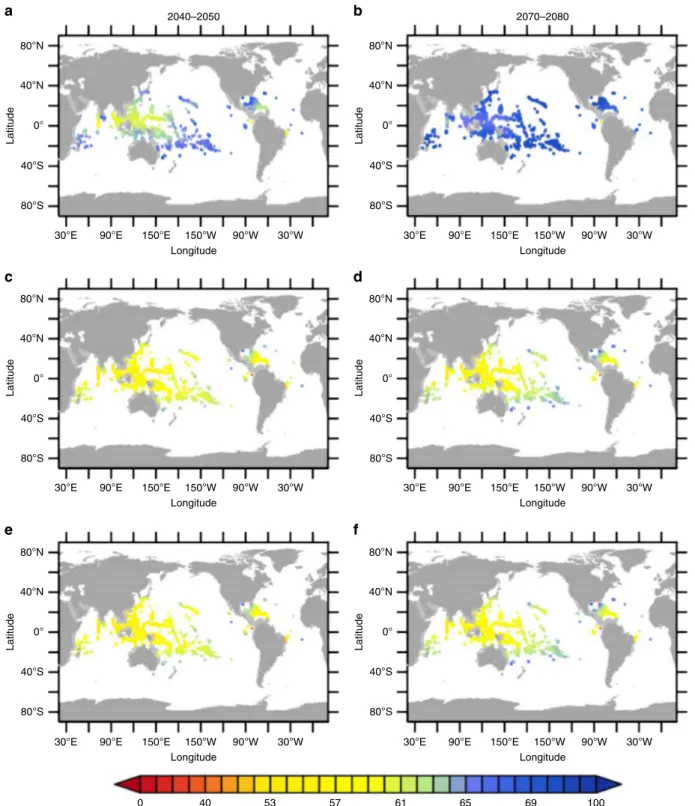
However, there are remarkable differences in the degree of damage among the different scenarios. In the case of EARLY (Fig. 6a), the gross community calcification rate TGgross in the Indonesian archipelago during 2040 to 2050 is projected to decline to 60–65% of its preindustrial value, while in LATE (Fig.6c) and SSP1-2.6 (Fig.6e), this value only reaches approximately 50–55%
of its former strength. Additionally, in the case of EARLY,TGgross in the tropical Pacific Ocean and Sargasso Sea declines to 65–70%
of its preindustrial value, while in case of LATE and SSP1-2.6,
TGgrossonly reaches 60% of its original value. During the seventies, a recognizable advantage of EARLY over LATE is even more pronounced (Fig. 6b, d, f). Coral reefs suffering from reduced biomineralization are at risk to grow malformed sceletons of higher porosity42. Although EARLY reveals only a 5–15%
improvement of calcification rates over LATE it might be of importance for the success of coral reefs to combat external stressors, such as ocean heat waves leading to bleaching events.
80°N
a b
c d
e f
40°N
LatitudeLatitudeLatitude
0°
40°S
80°S
30°E 90°E 150°E 150°W
Longitude Longitude
2040–2050 2070–2080
90°W 30°W 30°E 90°E 150°E 150°W 90°W 30°W
30°E 90°E 150°E 150°W
Longitude Longitude
90°W 30°W 30°E 90°E 150°E 150°W 90°W 30°W
30°E 90°E 150°E 150°W Longitude
0 40 53 57 61 65 69 100
Longitude
90°W 30°W 30°E 90°E 150°E 150°W 90°W 30°W
80°N
40°N
0°
40°S
80°S
80°N
40°N
0°
40°S
80°S
80°N
40°N
LatitudeLatitudeLatitude
0°
40°S
80°S
80°N
40°N
0°
40°S
80°S
80°N
40°N
0°
40°S
80°S
Fig. 6 Relative decadal mean gross calcification rates of tropical corals.Global distribution of tropical coral reefs from the Reef Base (M. Tupper et al., ReefBase: A Global Information System on Coral Reefs,http://www.reefbase.org) and their corresponding decadal mean gross calcification ratesTGgross relative to preindustrial values in %: (2040–2050)aEARLY;cLATE;eSSP1-2.6; (2070–2080)bEARLY;dLATE;fSSP1-2.6.
Discussion
Ocean acidification and climate change, as projected to occur by the mid-21st century, will pose a serious threat to marine biota, even under the most ambitious mitigation strategies (e.g., the SSP1-2.6 emission path). In this study, we focused on the impact of three ambitious scenarios of net CO2 emissons on living conditions for pteropods and tropical reef-building corals. Pter- opods play a significant role in the marine foodweb43, especially in polar regions. Our study found that large parts in the Arctic and Antarctic are expected to become uninhabitable for pter- opods, because severe acidification leads to large areas becoming seasonally undersaturated with respect to aragonite, which is the essential mineral needed for pteropod shells. Previous studies showed that changing water chemistry and temperature already have a negative impact on pteropod survival and shell formation18,44. As our model demonstrates, this trend is expected to continue over the next decades, but especially early CDR can prevent large areas in polar regions from becoming under- saturated with respect to aragonite and thus keep those areas habitable for pteropods.
The other important calcifiers highlighted in this study are tropical corals that are the foundation of major biodiversity hotspots in the ocean by providing habitat and resources to over a million reef-associated species14. Due to ocean acidification and warming, coral reefs are expected to become severely damaged12,45,46. Utilizing an empirical law for the effect of ocean acidification and warming on coral calcification by Silverman et al.41, our results suggest that even in the ambitious mitigation scenario SSP1-2.6 the calcification rate of corals will decrease to 50% of the preindustrial level. If, in addition to emissions reduction, CDR is deployed early, the calcification rates will be 5–15 percentage points higher. Reduced calcification rates imply that corals grow slower and have to spend more energy on cal- cification, which makes it harder for them to compete with macroalgae and seaweeds. This canfinally lead to a regime shift from a structurally complex and species-rich reef ecosystem to an algae-dominated ecosystem with lower biodiversity5,10,16.
It is important to mention that the future of a coral reef is not only determined by increasing open ocean pH and warming, which is calculated by our model, but also heavily influenced by local factors, such as the reef-specific buffer capacity of seawater, local currents and local overfishing and pollution47. To assess future developments of coral reef ecosystems further, regional model studies that can account for local pH variability and extremes are needed, whereas this study demonstrates the overall increasing pressure on coral reefs globally. According to our simulations, early deployment of CDR can contribute to the conservation of coral reefs on a global scale. Although some reefs are more resilient than others14,47, it is almost certain that in general the pressure on coral reefs will increase strongly with increasing atmospheric CO2 concentrations, resulting in chan- ging species composition, meaning that vulnerable coral species will be replaced by more resilient corals (e.g., species of thePorites genus)48–50or that in severe cases macroalgae will overgrow the whole reef. A global die-back of coral reefs would be accompanied by a loss of the associated ecosystem services that are important for coastal ecosystems like mangrove forests and human societies, e.g., coastal protection, tourism and food security10.
In this study, we demonstrated that in combination of reducing CO2 emissions rapidly, early deployment of atmospheric CDR measures could be effective in largely maintaining oceanic phy- sical and chemical conditions of today, provided the terrestrial carbon cycle remains a carbon sink until the end of the 21st century. Given the terrestrial carbon cycle would turn into a carbon source as suggested by a few model simulations34 provided by the Coupled Climate-Carbon Cycle Model
Intercomparison Project (C4MIP), an early deployment of atmospheric CDR measures would be much less effective (Sup- plementary Figs. 1 and 2 generated with modified parameters for the terrestrial submodel, see Supplementary Table 1). The latter indicates that the future development of the terrestrial biosphere is deeply connected with the marine biosphere and has the potential to accelerate the decrease of biodiversity in the ocean.
Accompanying aggressive climate mitigation pathways with CDR deployment at an early stage could help to dampen the most severe impacts on key marine ecosystems. To have a significant effect, though, it is crucial that CDR technologies are deployed as early as possible, ideally within the next decade.
Methods
CLIMBER-3α+C. The following describes the Earth system model employed and the experimental design of the simulations conducted. CLIMBER-3α+C is based on the EMIC51CLIMBER-3αwhich was described by Montoya et al.31in detail.
Since then, the model has been revised and extended with respect to its physical and biogeochemical components. In the following section, we present the most important innovations/modifications added to the original code.
Atmosphere. As its precursor, CLIMBER-3α+C still employs the statistic dynamical atmosphere POTSDAM-2 (Potsdam Statistical Dynamical Atmospheric Model 2)52, with a horizontal resolution of 7.5´ 22.5. The model realistically reproduces large scale structures, such as the Hadley circulation and the main high- and low-pressure systems, but does not resolve synoptic scale processes. The assumption of universal vertical structures of temperature and humidity allows for the reduction in their dynamic equations to a two-dimensional problem. The atmospheric wind velocities are provided at 10 different pressure levels. When calculating the longwave radiative transport, a 16 level scheme is employed31. The vegetation cover is prescribed as it is in the original version of CLIMBER-3α.
Because aeolian dust is one of the most important iron sources for marine biota, we have implemented an atmospheric dust transport model following Bauer and Ganopolski53. Similar to atmospheric humidity, it assumes an exponential vertical profile for the dust mixing ratiosMðzÞ:
MðzÞ ¼Msexpðz=hdÞ; ð1Þ
withhdrepresenting the scale hight of the dust mixing ratio (2000 m).Ms represents the near surface dust mixing ratio. If
ρðzÞ ¼ρsexpðz=haÞ ð2Þ
is the vertical profile of air density, with the atmospheric scale of highthaand near- surface density ofρs, then the vertically integrated dust concentration is given by:
D¼Z Ha zs
Mρdz ð3Þ
and the balance equation, which includes advective and diffusive transports, sources and sinks, reads:
∂D
∂t ¼ ∇H
Z Ha zs
ρ!uM dzZHa zs
ρK∇HM dz
!
þQRdRw; ð4Þ where
∇H¼!i ∂
∂xþ!j ∂
∂y ð5Þ
and!u represents the wind velocity vector.Qrepresents the dust emissionflux, which depends on the land surface type, erosion and the wind-dependent uplift of dust into the atmosphere53.RdandRwrepresent the dry and wet dust deposition rates, respectively. The parameters were taken from Bauer and Ganopolski53. Ocean general circulation model. CLIMBER-3α+C utilizes GFDL’s three dimensionalz-coordinate Modular Ocean Model (version 3.1) (MOM-3.1)54with the upgrades described in Hofmann and Maqueda55. This version benefits from the improved accuracy of a second-order moments advection scheme56which strictly limits spurious numerical diffusion and dispersion and employs a realistically low diapycnal background diffusivity of 105m2s1. Furthermore, the model accounts for the effects of geothermal heating57and a circulation dependent para- meterization of the Gent-McWilliams diffusivity58,59varying between 275 and 1100 m2s1in space and time. The models horizontal resolution is 3.75´3.75 while the vertical dimension is divided in 24 layers with thickness increasing with depth from 25 m at the top to a maximum of 514 m at the bottom. Save for the wind-stressfields, which are externally provided from a monthly mean climatol- ogy60, the OGCM exchanges radiative-, heat- and buoyancyfluxes with the atmosphere (POTSDAM-2) and the sea-ice model (ISIS)61. After a spin-up for more than 6000 years the model well reproduces the large scale pattern of
temperature and salinity while the maximum strength of the Atlantic meridional overturning circulation (AMOC) stabilizes at 14.4 Sv (1 Sv=106m3s1).
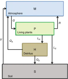
Terrestrial box model. CLIMBER-3α+C does not include a model of the ter- restrial biosphere. To, at least, emulate the response of the terrestrial carbon cycle to variations in atmospheric temperature and CO2concentration, a box model similar to that described by Wigley33was coupled with the atmospheric sub-model of CLIMBER-3α+C. The box-model comprises four boxes: (1) atmosphere (M), (2) living plants (P), (3) detritus (H) and (4) soil (S) (see Fig.7), which can exchange carbonfluxes among each other governed by the following equations.
dM
dt ¼IF ðGRQAUÞ ð6Þ
dP
dt¼GPRL ð7Þ
dH
dt ¼GHþLHQ ð8Þ
dS
dt¼GSþQSþLSU ð9Þ
HereIrepresents the anthropogenic net emission rate of CO2, andFrepresents theflux from the atmosphere to the ocean. The gross primary productionGis equal to the sum ofGP¼gPG,GH¼gLG, andGS¼ ð1gPgLÞG:G¼ GPþGHþGSandQrepresents the sum of the remineralizationfluxes from detritus to the atmosphere (QA) and soil reservoir (QS):Q¼QAþQS.Rrepresents the respirationflux from living plants into the atmosphere, andUrepresents the outgassing of soil due to remineralization. The carbonfluxLfrom dying plants can be written as the sum of thefluxes into detritus and the soil reservoir:LHþLS.
Following Wigley33thefluxesL,QandUcan be related to specific decay time constantsτ:L¼qPP=τP,Q¼qHSH=τH, andU¼qHSS=τS, while GP¼rmgPG0,R¼rmR0,GH¼rmgLG0,LH¼ΦL,QA=ð1λÞ Q, GS¼rm ð1gPgLÞ G0,QS=λQ, andLS=ð1ΦÞ L.
The temperature dependent quantitiesqPandqHSare given by:
qP¼ ðQP10ÞðTATM=10Þ ð10Þ
qHS¼ ðQHS10ÞðTATM=10Þ; ð11Þ with theQP10andQHS10factors given in Table1andTATMrepresenting the globally avaraged surface air temperature.
Given,Nrepresents the net primary production (NPP) at a given time andN0 represents the preindustrial NPP then62:
N
N0¼ðCCbÞð1þbðC0CbÞÞ
ðC0CbÞð1þbðCCbÞÞ¼rm; ð12Þ whereCis the atmospheric CO2concentration,C0=280 ppm, andCb=31 ppm
and
b¼ ð680CbÞ rð340CbÞ
ðr1Þð680CbÞð340CbÞ; ð13Þ The value forris given in Table1.
Tofind a parameter set for emulating the terrestrial biosphere under anthropogenic emissions during the late 21st century, we conducted several test runs, where we coupled the terrestrial box model with a simple box model of the ocean carbon cycle. Therefore, we were able to quickly run a large number of experiments with different model parameters. Thefinal parameter set derived from these experiments is listed in Table1.
Ocean carbon cycle and marine ecosystem models. The ocean carbon cycle and marine ecosystem model mainly bases on an upgraded version of the model by Six and Maier-Reimer63and prognostically solves for the spatio-temporal evolution of dissolved inorganic carbon (DIC), total alkalinity, phosphate, oxygen, silicate, phytoplankton, zooplankton, dissolved organic carbon (DOC), particulate organic carbon (POC), calcite, and dissolved iron. It assumes throughout a constant stoi- chiometric relationship between carbon (C), nitrate (NO3), phosphate (PO4), and oxygen (O2) of organic matter (Redfield-ratio63,64): C : NO3: H2PO4 : O2=122 : 16 : 1 : (−172)
The model is initialized with a homogeneous distribution of DIC (2341μmolL1), total alkalinity (2503μequL1), inorganic phosphate
(2.3μmolL1) and silicate (80.0μmolL1). We utilize the acidity constants given by Zeebe and Wolf-Gladrow (2002)65. Air-sea gas-exchange of CO2is parameterized according to Wanninkhof66as a quadratic function of the wind speed while oxygen fluxes are calculated from a simple restoring of sea surface concentrations to thermodynamically equilibrium values67. CLIMBER-3α+C accounts for the dynamics of dissolved iron by assuming only aeolian dust as the only source and including its co-limitation effects on the phytoplankton growth rates68as well as the mineral ballast effect69,70.
Experimental design. The base“SSP1-2.6”emission scenario starting in 2005 was linearly extended from year 2100 towards year 2150, where net emission rates were assumed to approach zero. To construct the emission scenario“EARLY”, we have subtracted annual CO2emission ratesf(t) from“SSP1-2.6”by imposing a logistic function between 2025 and 2050, where t represents the number of years.
fðtÞ ¼ L
1þexpðnLtÞðL1Þ ð14Þ
WithL=4.750 andn=0.2, CO2emission rates are assumed to drop to zero by year 2050. From here on, we assume zero net anthropogenic emission rates until the end of our simulations in year 2200. Within thefirst 25 years until the peak of the additional CDR is reached (2025–2050), an extra amount of 109 GtC is removed from the atmosphere. From 2050 until 2075 (i.e., until the time when the
“SSP1-2.6”scenario meets the zero emissions level), the“EARLY”scenario removes a further total of 59 GtC from the“SSP1-2.6”scenario which keeps net emissions at the zero line.
After 2075, the“SSP1-2.6”-emissions scenario reached net negative values on the order of−2.5 GtC yr1by the end of the 21st century. As a result,“SSP1-2.6”
requires total net negative emissions of 105 GtC between 2075 and 2150, while during the same period,“EARLY”assumes net zero emissions.
In constructing“LATE”, we used the same procedure based on the above logistic function. However, we applied the extra CDR measures 50 years later than those in the case of“EARLY”, starting in year 2075 and lasting until 2100.
To ensure the same additional cumulative carbon removal of 63 GtC relative to
“SSP1-2.6”in both the“EARLY”and“LATE”scenarios over the whole simulation time, we included a period of only mild net negative emissions after 2100 in the
“LATE”scenario, which linearly decreased to zero in 2150.
M
P
H
S Atmosphere
G
QA U
QS LH
R
LS Living plants
Detritus
Soil
Fig. 7 Terrestrial carbon cycle model.Box model of the terrestrial carbon cycle comprising the carbon pools and its exchangefluxes for the atmosphe (M), the living plants (P), the detritus (H) and the soil (S) (redrawn after Wigley33).
Table 1 Parameters for the terrestrial carbon cycle box model.
Parameter Value default Unit
G0 76 GtC year 1
R0 14 GtC year 1
QP10 1.4 —
QHS10 1.4 —
τP 60 years
τH 3 years
τS 400 years
Φ 0.98 —
gP 0.35 —
gL 0.6 —
r 1.4 —
λ 0.05 —