Introduction to R
Jens Schumacher May 7, 2012
R is a statistical computer program that is distributed under the GNU General Public Licence agreement. Among other things this means, that it is freely available (http://cran.r-project.org).
This does not yet qualify it as the statistics program of choice, but it certainly contributes to its popularity. A commercial product of similar flavour is S-Plus. Both programs are based on the programming language S and almost everything in this course can be done identically in S-Plus.
R offers an environment where you can do data management, graphics and statistical analysis.
The great strength of an open and flexible environment like R is the fact that you can use a wealth of predefined standard procedures and on the other hand you can relatively easy modify things to tackle particular problems. There is a worldwide community of R - users which steadily contributes to the functionality of R . Their contributions are organized in packages and you can use them in a modular fashion by just incorporating the packages you need. The appearance is quite different from the usual menu driven windows programs and for people not familiar with programming it may be somewhat daunting. But concerning user-friendliness let me cite Peter Dalgaard, the author of the book ”Introductory Statistics with R ”:
Whether R is user-friendly depends on the user... It does often have the advantage of actually being able to do what people need. If you can follow some simple examples, like those on the help pages, and do the relevant substitutions and modifications for your own problems, then you’re basically set. You can get quite far without actual programming. It’s something that is there for you when you need it.
1 A sample session
You can start the program using the Start-menu of the Windows-system (Start –>Programme –> R) . A relatively undecorated window opens with a command line prompt:
>
Ris an interactive system and commands are run immediately. But you can also write sequences of commands in a batch-file to process them in batch-mode.
1.1 Calculator
We expect a statistical computer program to be able to do basic calculations. And in fact R can do this. Addition:
> 3 + 5
[1] 8
Multiplication:
> 3 * 9 [1] 27
Division:
> 27/9
[1] 3
Integer Division:
> 137%/%19
[1] 7 Modulo:
> 137%%19
[1] 4
Exponentiation:
> 3^3
[1] 27
> 8^(1/3)
[1] 2
Beside these simple arithmetic functions there is a huge number of predefined mathematical functions. The probably most often used ones are summarized in table 1.
Table 1: Mathematical functions in R
Function Description
log(x) natural logarithm (base e= 2.71828...)
log10(x) logarithm to base 10
log(x,b) logarithm to base b exp(x) exponential function (ex)
sqrt(x) square root
choose(n,k) binomial coefficient n!/(k!(n−k)!)
gamma(x) gamma function (Γ(x) = (x−1)! for integern) lgamma(x) natural log of gamma function
floor(x) greatest integer< x ceiling(x) smallest integer > x
trunc(x) truncates all decimal places trunc=floor for positive values trunc=ceiling for negative values
round(x) rounding
round(x, digits=3) rounding to 3 decimal places cos(x) cosine of x (in radians)
sin(x) sine ofx (in radians)
tan(x) tangent ofx (in radians) acos(x),asin(x),atan(x) inverse trigonometric functions
abs(x) absolute value ofx
1.2 Short-term and long-term Memory
Getting a quick answer for a simple question and then forget about it is not what we usually ask for. We rather have more complicated questions and want to use the results for further analysis. Therefore, we need a way of keeping things in mind. To force R to keep something in short-term memory we need to assign a result to a named object using the assign operator ”<-”:
> result <- 3 * 27
In contrast to previous experience we don’t see anything happen now, but as long as we don’t quit our R - session we can now ask for the value stored in the object ”result”
> result
[1] 81
and we can use the value for any further calculation:
> result2 <- sqrt(result)
> result2
[1] 9
There is great freedom in the choice of names for R - objects. For small and quick task short names like x,y,f1,f2,... will be sufficient, for larger projects ”speaking” names are ad- visable. Usually people use the ”.”-notation known from object-oriented programming (soil- data.mehrstedt,soildata.kaltenborn,...) Some names are reserved to the R- system (like t,T,c,C,...) and you are not allowed to use underscores ” ” or (quite obviously) empty spaces in names.
Speaking names also reduce the danger of replacing the original content of an object (without warning!!!) when assigning a value to an object with the same name a second time. A list of all the currently known objects can be obtained by
> objects()
[1] "result" "result2"
You can clean up your workspace by removing objects from the list
> rm(result)
> objects()
[1] "result2"
Before you end an R- session you have to decide wether all the current objects should be moved into the long-term memory. You can do this using theFile-Save Workspacemenu, but you are also asked if you want to save the current workspace after typing
> q()
to quit the R - session. By default the objects are stored in a file ”.Rdata” which can be loaded again after you started a new R - session. Actually, if you start R by double-clicking on an .Rdata-file the working directory will be set to the current directory and all the objects stored will be available from the start. This allows organization of work on different projects in different directories with separate ”.Rdata” files. To switch between projects you can use thegetwd()(get working directory) and setwd()(set working directory) functions
> getwd()
[1] "O:/jschum"
> setwd("O:/jschum/¨Okonometrie")
or the File - Change dir menu. However quitting and restarting R is a better way to ensure that different projects are not mixed.
1.3 Vectors
The basic object for calculations in R is avector. Vectors are usually treated as column vectors (with some exceptions). The basic way to construct vectors in R is by just concatenating several numbers in one object using the c-function:
> x <- c(1.1, 3, 3.14159, 2.71828, 0)
> x
[1] 1.10000 3.00000 3.14159 2.71828 0.00000
There are several possibilities to define more regular sequences of numbers. A sequence of consecutive integers is obtained by
> 1:6
[1] 1 2 3 4 5 6
More general sequences can be created using the seq-function:
> seq(0, 1, by = 0.2)
[1] 0.0 0.2 0.4 0.6 0.8 1.0
The arguments of the function are the start value, end value and the step size. But how do we know that? It is not an easy task to keep all the arguments of the different functions in mind but the help-system of R provides immediate, informative guidance. To get help on a particular function we just type the functions name preceded by a question tag:
> ?seq
You get information about possible arguments, a more detailed description of the things hap- pening when the function is called, related help topics and examples. With some experience in R the examples often provide enough information on a functions most common usage and these can be directly accessed via
example(seq) seq>1:4 [1] 1 2 3 4
seq>pi:6 [1] 3.141593 4.141593 5.141593 seq>6:pi [1] 6 5 4
seq>seq(0, 1, length = 11) [1] 0.0 0.1 0.2 0.3 0.4 0.5 0.6 0.7 0.8 0.9 1.0 seq>str(seq(rnorm(20))) int [1:20] 1 2 3 4 5 6 7 8 9 10 ...
seq>seq(1, 9, by = 2) [1] 1 3 5 7 9
seq>seq(1, 9, by = pi) [1] 1.000000 4.141593 7.283185 seq>seq(1, 6, by = 3) [1] 1 4
...
1.4 Matrices
A matrix can be defined using thematrix() - function:
> (A <- matrix(1:12, 3, 4)) [,1] [,2] [,3] [,4]
[1,] 1 4 7 10
[2,] 2 5 8 11
[3,] 3 6 9 12
The second and third argument define the dimension of the matrix.
> dim(A)
[1] 3 4
> nrow(A)
[1] 3
> ncol(A)
[1] 4
By default the elements of the vector are entered column-wise. This can be changed by setting the argumentbyrowto true:
> (A <- matrix(1:12, 3, 4, byrow = T)) [,1] [,2] [,3] [,4]
[1,] 1 2 3 4
[2,] 5 6 7 8
[3,] 9 10 11 12
Whole columns or rows can be selected by omitting the second index:
> A[1, ]
[1] 1 2 3 4
> A[, 2]
[1] 2 6 10
Another way of defining matrizes is by combining different vectors either columnwise or rowwise:
> (x <- c(1, 3, 5))
[1] 1 3 5
> (eins <- rep(1, 3))
[1] 1 1 1
> cbind(eins, x) eins x [1,] 1 1 [2,] 1 3 [3,] 1 5
> rbind(eins, x) [,1] [,2] [,3]
eins 1 1 1
x 1 3 5
Note that for rbind the vectors are treated like row-vectors.
The usual arithmetic operators work elementwise:
> A + 1
[,1] [,2] [,3] [,4]
[1,] 2 3 4 5
[2,] 6 7 8 9
[3,] 10 11 12 13
> 3 * A
[,1] [,2] [,3] [,4]
[1,] 3 6 9 12
[2,] 15 18 21 24 [3,] 27 30 33 36
Multiplication of two matrizes of the same dimension is also done elementwise:
> (B <- matrix(rep(1:3, each = 4), 3, 4)) [,1] [,2] [,3] [,4]
[1,] 1 1 2 3
[2,] 1 2 2 3
[3,] 1 2 3 3
> A * B
[,1] [,2] [,3] [,4]
[1,] 1 2 6 12
[2,] 5 12 14 24
[3,] 9 20 33 36
True matrix multiplication uses the ’
> t(A) %*% B
[,1] [,2] [,3] [,4]
[1,] 15 29 39 45 [2,] 18 34 46 54 [3,] 21 39 53 63 [4,] 24 44 60 72
Here t(A)denotes the transpose of matrix A.
The inverse of a quadratic matrix is obtained by using the solve()-function:
> (C <- matrix(rnorm(9), 3, 3))
[,1] [,2] [,3]
[1,] -0.74706415 -0.16259296 0.60162401 [2,] -0.69101366 -0.32482209 0.77128237 [3,] -0.06886365 -0.08846669 -0.00616658
> (Cinv <- solve(C))
[,1] [,2] [,3]
[1,] -3.543492 2.735791 -3.532385 [2,] 2.894621 -2.322621 -8.095775 [3,] -1.955658 2.769453 -6.574262
1.5 Function arguments
The arguments given in parentheses when calling the function (0,1,0.2) are theactual arguments, whereasfrom, to, byandlengthareformal argumentsof the function. In the above function call the first actual argument 0 is matched to the formal parameterfrom, the second argument 2 to the formal argument to and the third actual argument to the formal parameterby. The third argument must be named, because there are two possible third arguments. The order of actual parameters can be arbitrarily changed, if the correct matching is ensured by giving the names of the formal arguments, e.g.
> seq(by = 0.2, to = 1, from = 0)
[1] 0.0 0.2 0.4 0.6 0.8 1.0
gives the identical result. Often the formal arguments have reasonable default values and can be omitted in the function call.
1.6 Vector arithmetic
Calculations using vectors are always done elementwise, which makes R a very efficient tool for data transformations. If, e.g.,
> needle.biom <- c(1.75, 4.81, 3.84, 3.44, 4.83, 0.72, 1.18, 1.49, 1.99, 1.72, 2.47, 3.27)
> needle.biom
[1] 1.75 4.81 3.84 3.44 4.83 0.72 1.18 1.49 1.99 1.72 2.47 3.27
is a vector consisting of needle biomasses of 12 spruce trees, the logarithmic values can be obtained by
> needle.logbiom <- log(needle.biom)
> needle.logbiom
[1] 0.5596158 1.5706971 1.3454724 1.2354715 1.5748465 -0.3285041 0.1655144 0.3987761 0.6881346 0.5423243 0.9042182 1.1847900 Similarly all the binary arithmetic operations work elementwise like
> x <- 1:10
> y <- c(seq(0, 0.5, by = 0.1), seq(0.5, 2, by = 0.5))
> x + y
[1] 1.0 2.1 3.2 4.3 5.4 6.5 7.5 9.0 10.5 12.0 Logical operators act elementwise as well:
> x > 5
[1] FALSE FALSE FALSE FALSE FALSE TRUE TRUE TRUE TRUE TRUE
Care has to be taken if vectors do not have the same length. In that case the shorter vector will be repeated until it is of the same length as the larger vector. This may or may not be the desired behaviour as in
> x + 1
[1] 2 3 4 5 6 7 8 9 10 11
adds 1 to each element of the vector. A warning message is given only if the length of the longer vector is no multiple of the smaller one:
> z <- c(1, 2, 3)
> x + z
[1] 2 4 6 5 7 9 8 10 12 11 Warning message:
longer object length is not a multiple of shorter object length in: x + z 1.7 Random numbers and summary statistics
R is also a powerful tool for doing statistical simulations. Many modern statistical analysis techniques (which we will not touch in this course) rely on extensive simulations.
The function
> sample(10)
[1] 9 4 3 8 10 2 1 7 6 5
results in a random shuffling of the numbers 1 to 10. Used with a second argument (size) this function can proof useful in randomly selecting a subsample of your data:
> sample(10, 5)
[1] 2 10 3 7 8
Ris also capable of generating random samples from several prespecified statistical distributions.
> x <- rnorm(100)
> x
[1] -0.083367170 0.525815486 -2.045664337 -1.844013211 [5] -0.132973581 -0.663347500 -0.128258485 -0.121907673 [9] 0.229635718 -0.732424675 -0.233975212 0.111073090 [13] -1.143215599 -0.328926233 -1.550480395 -1.353600105 [17] -0.261975790 0.484973645 -0.009635428 -0.151869347 [21] 1.287205447 0.951713187 -0.384971656 -1.938450224 [25] 1.040700636 0.542128584 -0.956624710 -0.410041084 ...
gives a random sample of 100 normally distributed random numbers whereas
> y <- rexp(100)
gives a sample of exponentially distributed random variables.
Simulating sample from specific distributions enables us to compare summary statistics of our sample with theoretical values. R has all the usual data summaries as predefined functions.
> sum(x)
[1] -12.97258
> mean(x) [1] -0.1297258
> median(x)
[1] -0.1366365
> var(x)
[1] 0.9472856
> sd(x)
[1] 0.973286
> quantile(x)
0% 25% 50% 75% 100%
-2.9174666 -0.7272682 -0.1366365 0.4131291 2.2260835
Skewness, a parameter used to describe the degree of asymmetry of a distribution, is not defined in the base package, but we can easily define our own function to calculate this data summary measure:
> skewness <- function(x) {
+ mean((x - mean(x))^3)/sd(x)^3 + }
This example shows how easily R can be extended by the user. Once we have defined the new function we can use it to calculate the skewness for any vector:
> skewness(x)
[1] -0.1639591
> skewness(y)
[1] 2.007378
Positive values (right-skew distributions) indicate that there are many small and few exception- ally large values
1.8 Data frames
Summarizing data in a few number of characteristics of their distribution constitutes part of descriptive statistics. When doing inferential statistics we study the relations between several variables measured on the same thing (individual, soil sample, ...) The vectors of values cor- responding to the different variables are usually put together in a data frame, a matrix-like object, where columns correspond to variables and rows correspond to individuals,...
The different variables may be of different type but have the same length.
> dataset <- data.frame(x, y)
> dataset
x y
1 -0.8574754 1.59503675 2 -0.3139234 0.86704582 3 -0.6005360 1.04677565 4 0.3178341 1.34635624 5 1.3006001 0.02907338
...
The columns of the data frame have got names, by default these are the names of the vectors combined in the data frame
> names(dataset)
[1] "x" "y"
but the can also be renamed
> names(dataset) <- c("norm", "exp")
The safest way to get data from ”abroad” into R is via .csv-files which can be produced, e.g., by Excel. These .csv-files contain the variable names in the first row and just numbers in all subsequent rows. You should give sensible column names already in Excel, R does not like empty spaces and underscores and including measurement units leads to awful column names in R . Import of data is realized by
> fatherandson <- read.csv("father&son.csv", sep = ";")
> names(fatherandson)
[1] "father" "son"
Small changes within a dataset can be done in a spreadsheet-like editor using
> edit(fatherandson)
but to make changes permanent we have to use the fix command
> fix(fatherandson)
Exporting data is possible using
> write.table(fatherandson, "fatherandson1.csv", sep = ";")
1.9 Indexing
Particular elements of vectors can be accessed using brackets by
> x[5]
[1] 1.3006
and this indexing can also be used to change single values
> x[5] <- 0
> x[5]
[1] 0
More than one element can be selected at the same time:
> x[1:3]
[1] -0.8574754 -0.3139234 -0.6005360
> x[c(2, 4, 6)]
[1] -0.3139234 0.3178341 -0.4649716 To select all positive values remember that
> x > 0
[1] FALSE FALSE FALSE TRUE FALSE FALSE TRUE FALSE FALSE FALSE TRUE TRUE FALSE FALSE ...
[26] TRUE FALSE FALSE FALSE TRUE FALSE FALSE FALSE FALSE TRUE FALSE FALSE FALSE FALSE ...
[51] FALSE FALSE TRUE TRUE FALSE TRUE FALSE TRUE FALSE TRUE TRUE TRUE FALSE TRUE ...
[76] TRUE TRUE TRUE TRUE TRUE FALSE FALSE FALSE FALSE TRUE FALSE TRUE TRUE FALSE ...
> positiv <- x > 0
gives a vector of TRUE and FALSE values. Using this vector we write
> x[positiv]
[1] 0.31783414 1.19014500 0.36351792 0.87230927 1.70930398 0.43301231 0.12246540 0.28688299 ...
[14] 0.08412040 0.60610657 1.61745331 0.90399070 0.86014254 0.26831375 0.17917676 1.56610529 ...
[27] 0.40539402 0.33357790 0.85252126 0.34219603 0.36588978 0.40650140 0.86122796 0.18726474 ...
[40] 0.86989617 0.12040629 0.90455915 0.39674766 0.26596644 0.16611869 0.12754598 or simply
> x[x > 0]
[1] 0.31783414 1.19014500 0.36351792 0.87230927 1.70930398 0.43301231 0.12246540 0.28688299 ...
[14] 0.08412040 0.60610657 1.61745331 0.90399070 0.86014254 0.26831375 0.17917676 1.56610529 ...
[27] 0.40539402 0.33357790 0.85252126 0.34219603 0.36588978 0.40650140 0.86122796 0.18726474 ...
[40] 0.86989617 0.12040629 0.90455915 0.39674766 0.26596644 0.16611869 0.12754598 Indexing a data frame is only slightly more complex. To select a single element you have to give the row and column index,
> fatherandson[1, 2]
[1] 1.66
gives the element in row 1 column 2. Whole row or columns can be extracted by leaving the other index blank
> fatherandson[1, ] father son
1 1.58 1.66
> fatherandson[, 1]
[1] 1.58 1.58 1.58 1.60 1.60 1.60 1.60 1.60 1.60 1.60 1.60 1.60 1.60 1.60 1.60 1.60 1.60 ...
[31] 1.62 1.62 1.62 1.62 1.62 1.62 1.62 1.62 1.62 1.64 1.64 1.64 1.64 1.64 1.64 1.64 1.64 ...
[61] 1.64 1.64 1.64 1.64 1.64 1.64 1.64 1.64 1.64 1.64 1.64 1.64 1.64 1.64 1.64 1.64 1.64 ...
...
A more convenient way of accessing the different variables in the data frame is provided by
> fatherandson$father
[1] 1.58 1.58 1.58 1.60 1.60 1.60 1.60 1.60 1.60 1.60 1.60 1.60 1.60 1.60 1.60 1.60 1.60 ...
[31] 1.62 1.62 1.62 1.62 1.62 1.62 1.62 1.62 1.62 1.64 1.64 1.64 1.64 1.64 1.64 1.64 1.64 ...
[61] 1.64 1.64 1.64 1.64 1.64 1.64 1.64 1.64 1.64 1.64 1.64 1.64 1.64 1.64 1.64 1.64 1.64 ...
...
which extracts a complete variable vector and can subsequently be indexed like a usual vector:
> fatherandson$father[5]
[1] 1.6
1.10 Graphics
The basic plotting command in R is plot, which is a so called generic function. Depending on the type of the argument is shows very different, but in most cases quite reasonable behaviour by ”guessing” what a potential user would like to see. When plotting a single vector, R plots the sequence of values
> plot(x)
Figure 1: Vector plot
●
●
●
●
●
●
●
●
●
●
●
●
●
●
●
●
●●
●
●
●
●
●
●
●
●
●
●
●
●
●
●
●
●
●
●
●
●
●
●
●●
●
●
●
●
●
●
●
●
●
●
●
●
●
●
●
●
●
●
●
●
●
●
●
●
●
●
●
●
●
●●
●
●
●
●
●
●
●
●
●
●
●
●
●
●
●
●
●
●
●
●●
●
●
●
●●●
0 20 40 60 80 100
−3−2−1012
Index
x
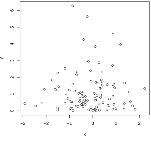
whereas for two vector arguments a scatterplot is produced
> plot(x, y)
We will see several variants of the plot function later on. The appearance of the default plots can be changed by passing additional arguments to the plot function or by changing the graphical parameters.
Figure 2: Scatterplot
●
●
●
●
●
●
●
●
●
●
● ●
●
●
●
●
●
●
●
●
● ●
●
● ●
● ●
●
●
● ● ●
●
●
●
●
●
●
● ●
●
● ●
●
●
●
●
●
●
●
●
●
●
● ●
●
●
●
●
●
●
●
●
●
●
●
●
●
●
●
●
●
●
●
● ●
●
●
●
●
●
●
●
●
●
●
●
●
●
●
●
●
●
●
● ●
●
●
●
●
−3 −2 −1 0 1 2
0123456
x
y
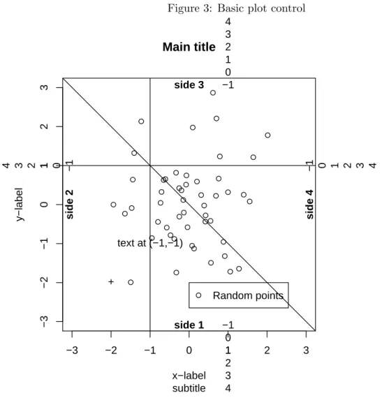
In principle everything is under user-control, but it takes some time to become familiar with all the options. The basics are summarized in the following figure:
> x <- rnorm(50)
> y <- rnorm(50)
> par(mar = c(5, 5, 5, 5))
> plot(x, y, main = "Main title", sub = "subtitle", xlim = c(-3, 3), ylim = c(-3, 3), xlab = "x-label", ylab = "y-label")
> abline(a = 0, b = -1)
> abline(h = 1, v = -1)
> points(-2, -2, pch = "+")
> text(-1, -1, "text at (-1,-1)")
> for (i in 1:4) mtext(-1:4, side = i, at = 1, line = -1:4)
> mtext(paste("side", 1:4), side = 1:4, line = -1, font = 2)
> legend(0, -2, "Random points", pch = 1)
Figure 3: Basic plot control
●
●
●
●
●
●
●
●
●
●
●
●
●
● ●
●
●
●
●
●
●
●
●
●
●
●
● ●
●
●
●
●
●
●
●●
●
●
●
●
●
●
●
●
●
●
●
●
●
●
−3 −2 −1 0 1 2 3
−3−2−10123
Main title
subtitle x−label
y−label
+
text at (−1,−1)
−1 0 1 2 3 4
−101234
−1 0 1 2 3 4
−1 0 1 2 3 4
side 1
side 2
side 3
side 4
● Random points
1.11 Using RStudio
Giving commands line by line at the command prompt is not very handy and very error-prone.
It is difficult to keep track of what has been done although we can move up and down the command history using the arrow keys and save all the submitted commands into a .history-file (a simple text file) using the File - Save history - menu. Recently RStudio was introduced as an integrated development environment (IDE) for R . This allows to write all R commands in a separate (commented) script file which can be saved as an ordinary text file, prefarably with extension.R. Shortcuts can be used to
send the current line or highlighted code to R :Ctrl + Enter)
execute the whole script : Ctrl + Shift + Enter
Apart from having all things well organized on the screen the main advantage is probably the possibility to get online help for function arguments: Tab or Ctrl + Space