Accepted Article
F. Hansen,
a∗R. J. Greatbatch,
a,bG. Gollan
a, T. Jung
c,dand A. Weisheimer
e,faGEOMAR Helmholtz Centre for Ocean Research Kiel, Kiel, Germany
bFaculty of Mathematics and Natural Sciences, University of Kiel, Kiel, Germany
cAlfred Wegener Institute, Helmholtz Centre for Polar and Marine Research, Bremerhaven, Germany
dDepartment of Physics and Electrical Engineering at the University of Bremen, Bremen, Germany
eDepartment of Physics, National Centre for Atmospheric Science (NCAS), University of Oxford, Oxford, UK
fEuropean Centre for Medium-Range Weather Forecasts (ECMWF), Reading, UK
∗Correspondence to: GEOMAR Helmholtz Centre for Ocean Research Kiel, Duesternbrooker Weg 20, 24105 Kiel, Germany.
E-mail: fhansen@geomar.de.
The phase and the amplitude of the North Atlantic Oscillation (NAO) are influenced by numerous factors, which include Sea Surface Temperature (SST) anomalies in both the Tropics and extratropics and stratospheric extreme events like Stratospheric Sudden Warmings (SSWs). Analyzing seasonal forecast experiments, which cover the winters from 1979/80–2013/14, with the European Centre for Medium-Range Weather Forecast model, we investigate how these factors affect NAO variability and predictability.
Building on the idea that the tropical influence might happen via the stratosphere, special emphasis is placed on the role of major SSWs. Relaxation experiments are performed, where different regions of the atmosphere are relaxed towards ERA-Interim to obtain perfect forecasts in those regions. By comparing experiments with relaxation in the tropical atmosphere, performed with an atmosphere-only model on the one hand and a coupled atmosphere-ocean model version on the other, the importance of extratropical atmosphere-ocean interaction is addressed.
Interannual variability of the NAO is best reproduced when perfect knowledge about the NH stratosphere is available together with perfect knowledge of SSTs and sea ice, in which case 64% of the variance of the winter mean NAO is projected to be accounted for with a forecast ensemble of infinite size. The coupled experiment shows a strong bias in the stratospheric polar night jet (PNJ) which might be associated with a drift in the modelled SSTs resembling the North Atlantic cold bias and an underestimation of blockings in the North Atlantic/Europe sector. Consistent with the stronger PNJ, the lowest frequency of major SSWs is found in this experiment. However, after statistically removing the bias, a perfect forecast of the tropical atmosphere and allowing two-way atmosphere-ocean coupling in the extratropics seem to be key ingredients for successful SSW predictions. In combination with SSW occurrence, a clear shift of the predicted NAO towards lower values occurs.
Key Words: North Atlantic Oscillation; stratosphere; predictability; seasonal forecast; tropical influence; atmosphere- ocean coupling.
Received . . .
1. Introduction
The North Atlantic Oscillation (NAO) is responsible for a large part of the atmospheric variability in the North Atlantic/Europe sector. Accounting for more than 30% of the variability of winter mean surface air temperature in the Northern Hemisphere (NH) (Hurrell 1996), it is a major driver of European winter weather and
climate. An equivalent barotropic, predominantly tropospheric phenomenon, a positive NAO phase, is associated with below- normal geopotential height (GPH) and sea level pressure (SLP) centred near Iceland and above-normal GPH and SLP centred over the Azores. This configuration favours a stronger westerly circulation and results in milder and wetter winters in Northern and central Europe, while a negative NAO phase has the opposite
This article has been accepted for publication and undergone full peer review but has not been through the copyediting, typesetting, pagination and proofreading process, which may lead to differences between this version and the Version of Record. Please cite this article as doi: 10.1
002
/qj.2958
This article is protected by copyright. All rights reserved.
Accepted Article
effect (Hurrell 1995; Greatbatch 2000; Hurrellet al.2003). Due to its high significance for European winter weather and climate, and the resulting socio-economic implications, the NAO has been extensively studied in the last decades, and attempts have been made to predict the seasonal NAO phase tendency several months ahead. A successful NAO prediction depends on knowledge about the factors which influence its phase and amplitude. Often mentioned in this context is the influence of surface conditions like snow cover over the Eurasian continent during autumn (Cohen and Entekhabi 1999); the extent of Arctic sea ice (Wu and Zhang 2010); sea surface temperature (SST) anomalies in the North Atlantic, e.g. the appearance of the North Atlantic SST tripole (Ratcliffe and Murray 1970; Rodwell and Folland 2002; Taws et al.2011; Maidenset al.2013); SST anomalies in the tropical Pacific, in particular in association with the El Ni˜no-Southern Oscillation (ENSO) (Fraedrich and Muller 1992; Hoerlinget al.
2001; Greatbatchet al.2004; Greatbatch and Jung 2007; Ineson and Scaife 2009; Bellet al.2009); the Madden-Julian Oscillation (Cassou 2008; Linet al.2009, 2015); general conditions in the NH stratosphere, notably the state of the stratospheric polar vortex and the occurrence of stratospheric extreme events, so called major stratospheric sudden warmings, perhaps in association with the Quasi-Biennial Oscillation (QBO) in the equatorial stratosphere (e.g. Holton and Tan 1980, 1982; Pascoeet al.2006; Boer and Hamilton 2008).
In this paper, we focus on the importance of the Tropics, and the link to the stratospheric state, for NAO variability and predictability, building on the idea that the tropical SST influence on the North Atlantic might happen via a pathway through the stratosphere (Ineson and Scaife 2009; Bell et al.
2009; Butler et al. 2014). The Tropics have been found to be important for the North Atlantic/European climate in some outstanding winters e.g. in terms of extreme surface temperatures, notably 1962/1963 (Greatbatch et al. 2015), 2005/2006 (Jung et al. 2010b), 2009/2010 (Fereday et al. 2012) or 2013/2014 (Huntingford et al. 2014). A general impact could be shown by Greatbatch et al. (2012) for the NAO trend and interannual variability between 1960 and 2002. The proposed mechanisms include the idea of a Rossby wave train being excited in the tropical Pacific and redirected towards the North Atlantic and
European region (Gollan and Greatbatch 2015; Greatbatchet al.
2015), which is influenced by the winds in the upper equatorial troposphere and the stratosphere, where the latter are dominated by the phase of the QBO (Gollan and Greatbatch 2015). Other studies (Ineson and Scaife 2009; Bellet al. 2009; Butler et al.
2014) highlight the importance of the stratosphere in acting as a bridge between anomalies in tropical Pacific SSTs, mainly due to ENSO, and Europe. Manzini et al. (2006), Ineson and Scaife (2009) and Ayarzag¨uena et al. (2013) suggested that the large-scale, extratropical El Ni˜no teleconnection pattern in NH winter, which includes a deepening of the Aleutian low (e.g. Trenberth et al. 1998), enhances the forcing and vertical propagation of quasi-stationary planetary waves, resulting in a weaker stratospheric polar vortex. Over Europe, this results in a late winter surface pressure pattern resembling the negative NAO phase (Huang et al. 1998; Toniazzo and Scaife 2006;
Broennimannet al.2007; Broennimann 2007; Ineson and Scaife 2009), with cold and dry conditions over Northern Europe, and mild and wet conditions over Southern Europe.
Surface influence from the stratosphere is mainly observed after major SSWs. During these events, the stratospheric polar vortex is disturbed in such a way that the temperatures can increase by up to several tens of◦C within a few days, and the climatological westerly winds in the stratospheric polar night jet reverse to easterly. Major SSWs occur about every second winter (Erlebach et al.1996; Labitzke and Naujokat 2000; Charltonet al.2007).
Their signatures can descend down to the troposphere, with the resulting surface pattern projecting onto the negative phase of the NAO and hence affecting surface weather and climate (Quiroz 1977; Baldwin and Dunkerton 2001; Thompsonet al.2002; Scaife et al.2005; Charltonet al.2007; Douville 2009; Mitchellet al.
2013; Sigmondet al.2013). Greatbatchet al.(2015) argue that the SSW at the end of January 1963 extended the severe weather that winter into February, Scaife and Knight (2008) find in a model study with an artificially induced SSW that the January 2006 SSW probably contributed to the cold winter of 2005/2006, and Fereday et al. (2012) highlight the importance of the major warming in January 2010 in the dynamics of the winter of 2009/2010, when the NAO index was at a record low. In a recent study by Scaifeet al.(2016) using the Met Office Global forecast system,
This article is protected by copyright. All rights reserved.
Accepted Article
a system which has successfully been used for NAO seasonal predictions (Scaifeet al. 2014), the authors found a significant shift of the NAO phase towards more negative values after SSWs.
When members of the ensemble forecasts containing SSWs were excluded, NAO prediction skill vanished.
The present study has two main objectives: we first analyze briefly whether or not the general influence of the Tropics and the stratosphere on the NH winter NAO detected for the period 1960–2002 in Greatbatch et al. (2012) has changed in more recent years. In a second step, we want to focus on the role of major SSWs for NAO variability and prediction, and on the question what role the Tropics, and coupling between the ocean and the atmosphere, play in this context. For our analysis, we have performed ensemble seasonal forecast experiments with the European Centre for Medium-Range Weather Forecast (ECMWF) model, similar to Jung et al. (2010b, 2011) and Greatbatch et al. (2012). In these experiments we have used a relaxation technique where different parts of the atmosphere in the model are relaxed towards reanalysis data. This technique allows us to obtain “perfect forecasts” for the relaxed regions and hence, by comparing experiments with and without relaxation, to learn something about the importance these regions have for our region of interest, the North Atlantic and Europe. To address the question of the importance of atmosphere-ocean coupling, we compare experiments using the ECMWF atmosphere-only model, on the one hand, with experiments using the ECMWF coupled model on the other.
The paper is structured as follows: Section 1 provides information about the ECMWF atmosphere model(s) used in this study, the relaxation technique and the experiments that have been performed. In the same section, the NAO index and the definition used for a major SSW are introduced. Sections 2–4 present the results, first providing an overview of the global prediction skill in the different relaxation experiments, then focusing on the importance of the Tropics and the stratosphere for the NAO prediction skill and how this has changed in recent years, by comparing to the results obtained in Greatbatch et al. (2012), and finally discussing the role of the Tropics, ocean-atmosphere coupling and SSWs for NAO variability and prediction. The paper closes with a summary and discussion of the results.
1.1. Model and experiments
The model used in this study is the ECMWF model in two different setups: first the ECMWF Integrated Forecast System (IFS), an atmosphere-only model, with SSTs and sea ice prescribed at the lower boundary (varying between different experiments; see below), and second a coupled model version where the atmospheric model is coupled to the NEMO ocean model. The atmospheric model in both model versions is run in its cycle CY40R1 at spectral truncation T255 with 60 levels in the vertical, extending up to 0.01 hPa. The horizontal and vertical resolution used here are the same as for the ERA-Interim reanalysis (Dee et al. 2011). The NEMO model is run at 1◦ horizontal resolution with higher resolution near the Equator. Detailed model descriptions of the IFS model in its cycle CY40R1 can be found here https://software.ecmwf.int/wiki/display/IFS/CY40R1+Official+
IFS+Documentation.
Ensemble seasonal forecast experiments were performed with the two model versions, initialized each year around the beginning of November during the ERA-Interim period (1979–2013;
1981–2013 for the coupled model experiment) and run until the end of February of the same winter. Initial conditions and SSTs and sea ice for lower boundary conditions were taken from the ERA-Interim reanalysis. For the atmosphere-only experiments, 9 ensemble members were computed for each experiment, where the ensemble members were created using a lagged time approach with the initial and boundary conditions being chosen from 6 hourly intervals between November 1st 00 UTC and November 3rd 00 UTC. For the coupled-model experiment, 28 ensemble members were created as described in Watsonet al.(2016).
To investigate the respective importance of different parts of the atmosphere (Tropics, stratosphere...) for our region of interest, these specific parts of the atmosphere were relaxed towards ERA-Interim reanalysis in the course of the simulation, as was done in Jung et al.(2010b, 2011) and Greatbatch et al.(2012) using the ERA40 reanalysis; see also Watsonet al.(2016). In this way, “perfect forecasts” are created for these regions. Readers are referred to the papers by Junget al.(2010b,a) and Hoskins et al. (2012) for more discussion on the relaxation technique.
This article is protected by copyright. All rights reserved.
Accepted Article
Relaxation was done on the dynamic variables horizontal velocity, temperature, surface pressure (not for the experiments with stratospheric relaxation; see below), and additionally specific humidity and related parameters in the coupled experiment, with a time-scale of 10h in the atmosphere-only experiments, and a time-scale of 2h 45min in the coupled experiment.
The following experiments were performed for this study:
• CLIM-NO: Climatological SSTs and sea ice are prescribed at the lower boundary in this simulation. The climatology is computed for the whole ERA-Interim period. No relaxation is applied here. Information about a particular winter is present only in the initial conditions.
• OBS-NO: Observed SSTs and sea ice are prescribed at the lower boundary; no relaxation is applied.
• CLIM-TROPICS: Climatological SSTs and sea ice are prescribed at the lower boundary. Relaxation is applied over the whole depth of the atmosphere in the Tropics between 20◦S and 20◦N. These latitudes indicate the centres of 20◦ wide transition zones where the relaxation coefficient is changing from zero to full relaxation by a hyperbolic tangent function to obtain a smooth transition between relaxed and unrelaxed regions.
• OBS-TROPICS: Observed SSTs and sea ice are prescribed at the lower boundary, and relaxation is applied in the Tropics over the whole depth of the atmosphere, as in CLIM-TROPICS. Comparing the output of this experiment to CLIM-TROPICS, conclusions can be drawn about the influence of extratropical SSTs and sea ice as the two experiments are virtually identical in the Tropics where the strong intervention by the relaxation overwhelms the specification of SSTs.
• CPL-TROPICS: The NEMO ocean model is coupled to the atmosphere in this simulation. Relaxation is applied in the Tropics over the whole depth of the atmosphere as in CLIM-TROPICS and OBS-TROPICS. As the atmospheric relaxation is assumed to dominate any effect from SSTs in the relaxed region, differences between CPL-TROPICS and OBS-TROPICS can be interpreted as the effect of having interactive atmosphere-ocean coupling in the extra-tropics.
• CLIM-STRAT: Climatological SSTs and sea ice are prescribed at the lower boundary. Relaxation is applied in the NH stratosphere north of 20◦N and roughly above 100hPa, using a smooth transition function as in Junget al.
(2010a, 2011).
• OBS-STRAT: Observed SSTs and sea ice are prescribed at the lower boundary, and relaxation is applied in the stratosphere as in CLIM-STRAT.
1.2. NAO
The NAO index in this study is defined similar to that in Hurrell et al. (2003) as the Principal Component of the first Empirical Orthogonal Function (EOF) of GPH winter mean (December through February; DJF) anomalies at 500hPa in the North Atlantic sector (30–80◦N, 90◦W–40◦E). In this context, “anomalies” for each winter are computed separately for each experiment and for each ensemble member with respect to the winter average over all winters and all ensemble members for that particular experiment. To obtain the NAO index for the model simulations, the modeled winter mean anomalies are projected onto the EOF pattern obtained from ERA-Interim reanalysis data, and the resulting index is divided by the standard deviation of the observed NAO index. In this way, a misinterpretation of the results due to potentially different climatologies in the different model experiments is avoided. The main results of this study are not sensitive to the NAO index definition and do not change if the NAO index is defined at the surface as defined by Hurrell (1995).
1.3. Major Stratospheric Sudden Warmings
The definition of major SSWs follows the original definition of the World Meteorological Organization. According to this definition, a major SSW occurs when between November and April (1) the zonal mean zonal wind at 60◦N, 10 hPa reverses from its climatological (in winter) westerly direction to easterly, i.e., a breakdown of the stratospheric polar night jet occurs, and (2) the temperature gradient between 60 and 90◦N is positive for at least five days in the period from 10 days before to 4 days after the day of the wind reversal, referred to as the central date of the event hereafter (Labitzke and Naujokat 2000). No second event can be defined within 20 days after a central date; instead, any (obviously
This article is protected by copyright. All rights reserved.
Accepted Article
small) fluctuations during this period are counted as one event.
Using this definition, a total number of 18 major SSWs can be identified in ERA-Interim between 1979 and 2013.
In the ERA-Interim reanalysis, we also classify so-called final warmings which indicate the return to the easterly summer circulation. Final warmings fulfill the same conditions as major warmings, but the winds do not return to westerlies after the event and before the end of April for more than 10 days. As the forecast experiments only run until the end of February, we cannot identify final warmings for them.
2. Predictive skill in relaxation experiments
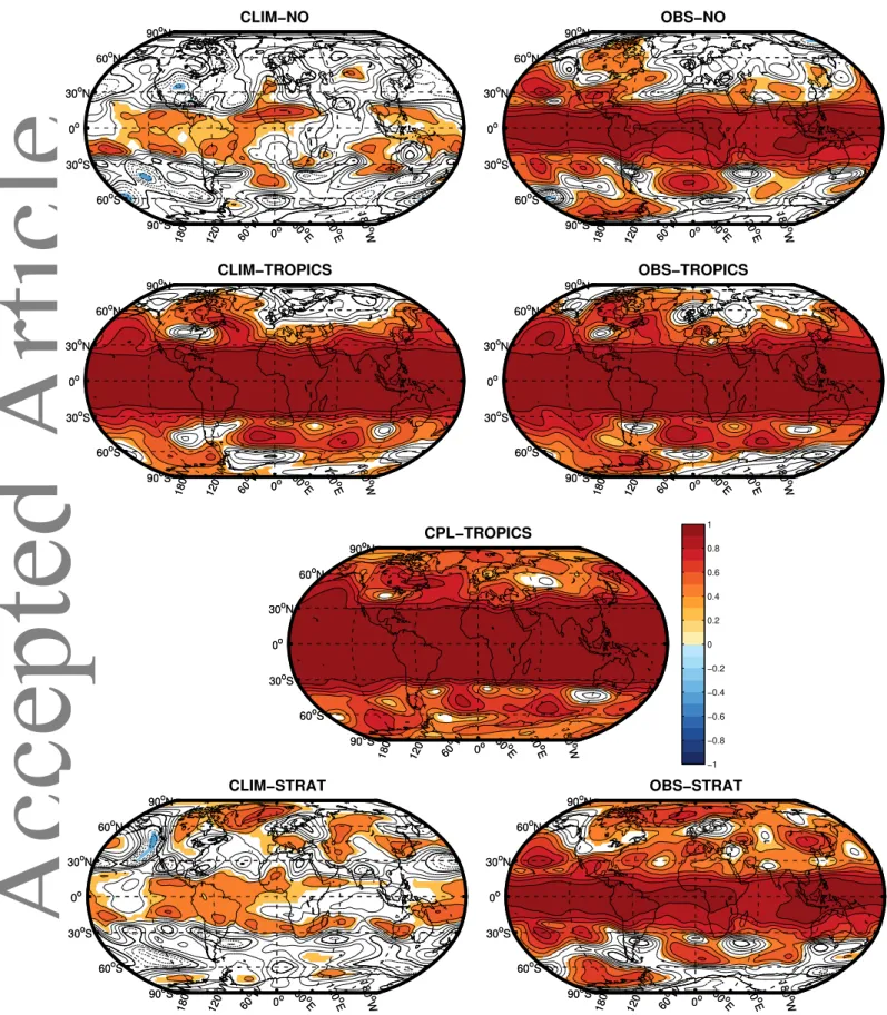
As a first step, we address the global predictive skill of the model in the different relaxation experiments. To do that, we analyze the Anomaly Correlation Coefficient (ACC) for GPH at 500hPa (GPH500) at each grid point. The ACC quantifies the correlation between forecast and observed deviations from climatology, with an ACC of one meaning a perfect prediction, and an ACC of zero or less denoting no predictability of the forecast system at that grid point.
Figure 1 shows the ACC in the different experiments compared to ERA-Interim. For the experiments, the DJF anomalies of the ensemble means are correlated with ERA-Interim anomalies. As expected, almost perfect predictive skill can be found in the Tropics between 30◦S and 30◦N in the three tropical relaxation experiments. The high ACC in the inner Tropics in OBS-NO, where observed SSTs are prescribed globally and no relaxation is used, shows that a successful prediction for this region depends to a large extent on having correct oceanic boundary conditions.
Some of the GPH500 skill in the Tropics is found even when specifying climatological oceanic conditions as can be seen from the significant ACC in CLIM-NO and CLIM-STRAT, where the lower boundary forcing consists of climatological SSTs and sea ice. This is particularly true for the western and eastern tropical Pacific, for Middle America and northern South America and for the tropical Atlantic, especially along the NH subtropical jet.
In CLIM-NO this indicates memory from the initial conditions specified at the beginning of November. Generally speaking, the differences between CLIM-NO and CLIM-STRAT in the Tropics
are small, indicating that most of the skill in the Tropics in CLIM- STRAT is coming from the initial conditions as well.
In the Extratropics, significant skill arises from relaxing the tropical atmosphere. In the NH, this skill is particularly pronounced over the North Pacific which can probably mostly be assigned to ENSO teleconnections (e.g. Trenberth et al.
1998). A significant ACC of more than 0.8 can also be found over the central and western North Atlantic, extending over northern North America, in all tropical relaxation experiments, whereas the predictive skill decreases towards the eastern North Atlantic and Northern Europe in these experiments. No skill in GPH500 is found over the British Isles and Scandinavia in CLIM-TROPICS and OBS-TROPICS. An improved skill due to varying extratropical SSTs (OBS-TROPICS compared to CLIM- TROPICS) is found over large parts of the NH where skill is observed from the Tropics anyway (CLIM-TROPICS), and additional significant prediction skill arises in the Greenland- Norwegian Sea region. Using an interactively coupled ocean model instead of prescribed SSTs and sea ice at the lower boundary (CPL-TROPICS) seems to increase the predictive skill over large parts of the NH and also over the North Atlantic and Europe. Whether or not this automatically means better predictions for the NAO will be further investigated in the following sections.
When the stratosphere is relaxed in the course of the forecasts (CLIM-STRAT), significant skill beyond that in CLIM-NO is most pronounced over Greenland and Iceland, i.e. the northern centre of action of the NAO, central northern North America as well as central and southern Europe. The effect of observed versus climatological SSTs (OBS-STRAT compared to CLIM-STRAT) more or less seems to add linearly, combining the skill in OBS- NO with that in CLIM-STRAT.
3. NAO skill in the different experiments
In a next step, we focus more on our region of interest, the Euro-Atlantic sector, and investigate from which regions skill for NAO predictions might result. We repeat parts of the analysis Greatbatchet al.(2012) have performed for the period 1960/61 to 2001/02 covered by ERA40 and compute the NAO index for each of our experiments, covering the more recent ERA-Interim
This article is protected by copyright. All rights reserved.
Accepted Article
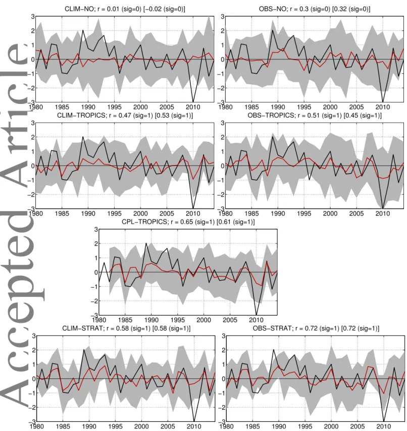
period. It has to be noted that the latter benefits from an improved data stream due to available satellite data after around 1979, and that our ERA-Interim experiments have been performed with a later model version having somewhat higher resolution (T255 compared to T159). Like Figure 2 in Greatbatchet al.(2012), the red line in Figure 2 shows the NAO index for the ensemble mean of the experiments, and the grey shading gives the range of the ensemble mean time series +/- two standard deviations to see if the observed index (given by the black line) is represented within the spread of model realizations. The numbers above each panel are the correlation coefficients between modeled and observed index, with the correlation coefficients of the detrended time series in brackets.
As in Greatbatch et al. (2012), we see that even in CLIM- NO, the experiment without any relaxation and where only climatological SSTs and sea ice are used at the lower boundary, the observed NAO index is a possible realization of the experiment as it does not exceed the range of 2 standard deviations around the ensemble mean (aside from a few exceptions, notably the extreme negative NAO winter of 2009/2010). But instead of the slightly significant negative correlation that Greatbatchet al.
(2012) found between the observed (ERA40) and the CLIM- NO NAO index, we see no correlation between our CLIM- NO ensemble mean realization and ERA-Interim for the recent decades, supporting Greatbatch et al. (2012)’s conclusion that their marginally significant correlation was “fortuitous”. These results nevertheless appear to contradict those of Stockdaleet al.
(2015) who claim to have found forecast skill using the ECMWF seasonal forecast system for the winter Arctic Oscillation that arises from the initial conditions alone, an issue that requires further investigation.
Apart from that, we find significant positive correlations between observed and modeled NAO time series in all three experiments using relaxation in the Tropics as well as both stratospheric relaxation experiments, for the undetrended and detrended time series. As in Greatbatchet al. (2012), the temporal variance of the ensemble mean NAO time series is considerably smaller than the observed one. In this respect, it does not seem to make a difference if observed SSTs or a coupled ocean model is used at the lower boundary, although the coupled model version seems
to reproduce the observed variability better than the atmosphere- only version using observed SSTs and sea ice (correlation of 0.65 (detrended: 0.61) with ERA-Interim in CPL-TROPICS compared to 0.51 (0.45) in OBS-TROPICS). The correlation between the OBS-TROPICS and CPL-TROPICS NAO indices is 0.68 (0.63 for the detrended time series), and the difference in correlation coefficient with ERA-Interim might at first sight seem large. However, having a closer look at the representation of individual years in the two experiments and especially at the major peaks, no large differences occur: both model versions have problems to reproduce the extreme positive NAO winters of 1988/1989, 1991/1992 and 1992/1993, with the latter two probably being an underestimated response to the eruption of Mt.
Pinatubo in 1991 (see e.g. Stenchikov et al. (2004); Marshall et al. (2009) for the NAO response to volcanic eruptions in climate models). CPL-TROPICS reproduces noticeably better the negative NAO in 1995/1996, and in the shorter time series (the coupled experiment was only started in 1981 compared to 1979 in the atmosphere-only runs) this already serves as a part of the explanation for the higher correlation with ERA-Interim: with the winter 1995/1996 left out, the correlation of OBS-TROPICS with ERA-Interim increases to 0.56, while it stays about the same (0.64) in CPL-TROPICS. Interestingly, in all experiments using tropical relaxation the model captures the tendency towards the extreme negative NAO in winter 2009/2010; however, only in the experiment using observed SSTs (OBS-TROPICS) does the extreme observed amplitude sit within the spread of modeled NAO values. This might support the idea from Jung et al.
(2011) that internal variability played a role for the negative NAO in that winter, but on the other hand our experiments also indicate a clear role from the Tropics and even the stratosphere, a role which had been suggested by Fereday et al.(2012) but which had been ruled out in Junget al. (2011). For the winter 2010/2011, which experienced an outstanding December in terms of extremely cold surface temperatures in Europe, our results suggest an influence from extratropical SSTs and sea ice, as the tendency towards the negative NAO is represented correctly only in OBS-TROPICS, but not in the relaxation experiments without tropical relaxation, nor in CLIM-TROPICS, nor in the stratospheric relaxation experiments. That means that our results
This article is protected by copyright. All rights reserved.
Accepted Article
are consistent with the suggestion of Taws et al. (2011) who claim that the negative NAO in 2010/2011 was related to the re-emergence of SST anomalies in the North Atlantic from the previous extreme NAO winter. The results are also in line with Maidens et al. (2013) who find anomalous heat content and associated SST anomalies in the North Atlantic being the key ingredients for a successful forecast of December 2010.
The NAO variability is best reproduced in the experiment that uses a combination of relaxation in the stratosphere and observed SSTs and sea ice at the lower boundary (OBS-STRAT; correlation of 0.72 with ERA-Interim) which - in comparison with OBS- NO - highlights the importance of a correct representation of stratosphere-troposphere coupling in the model for the dynamics in the North Atlantic region.
Overall, in comparison with Greatbatchet al.(2012), the results here suggest that the influence of the Tropics and the stratosphere on NAO interannual variability have not changed significantly in recent years (i.e. the ERA-Interim period) compared to an earlier period (i.e. the ERA40 period). When comparing our results to Greatbatchet al.(2012), it has to be kept in mind that the model version used here is more advanced than in Greatbatch et al.
(2012) and uses a higher horizontal resolution (T255 compared to T159).
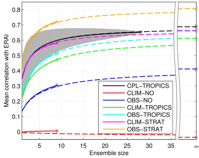
Another constraint when interpreting the results above is provoked by the different ensemble sizes of the experiments (9 ensemble members in the uncoupled experiments, and 28 members in CPL- TROPICS). Due to its greater ensemble size, CPL-TROPICS is likely to contain less noise than the uncoupled experiments, and hence correlate better with ERA-Interim. To address the question of how the ensemble size affects the NAO skill, we have computed the NAO correlation skill of the different experiments (i.e. correlations with ERA-Interim) as a function of ensemble size after Scaife et al. (2014), shown in Figure 3. The solid curves in Figure 3 show the average of correlations between all possible ensemble mean combinations created from the existing 9 (CPL-TROPICS: 28) ensemble members for each ensemble size (1:9; 1:28 for CPL-TROPICS) and ERA-Interim. These curves naturally end at the correlation value for the full ensemble that is shown in Figure 2. The dashed curves give a theoretical estimate of the variation of the NAO correlation with the ensemble
size following Murphy (1990). The solid curves follow the theoretical estimates very closely for most experiments, with the exception of CLIM-NO, where no NAO skill was found anyway.
From the asymptotes of the theoretical estimates we can see that even with an ensemble of infinite size, the NAO skill in CPL-TROPICS would still be higher than in the other tropical relaxation experiments which confirms the results described above. Interestingly, although larger differences in the NAO skill are found before between CLIM-STRAT and OBS-TROPICS than between OBS-TROPICS and CLIM-TROPICS (see asterisks) for an ensemble mean created of 9 ensemble members, for an infinite ensemble size CLIM-STRAT and OBS-TROPICS would have more or less the same skill. That means that increasing the ensemble size has the largest effect in OBS-TROPICS, which again indicates that the signal-to-noise ratio is comparably low in this experiment. The asymptote of OBS-STRAT tells us that we would expect up to 64% of the winter NAO variance to be explained when perfect knowledge of the stratosphere together with SST and sea ice is available in a forecast ensemble of infinite size, leaving another 36% to be probably explained by internal atmospheric dynamic processes. Notably, the experiment in which only the observed time series of SST and sea ice is specified, with no relaxation, gives by far the worst performance apart from CLIM-NO indicating that model error can result from specifying SST and sea ice alone. Adding stratospheric relaxation, as in OBS- STRAT, clearly goes some way towards correcting this error, at least for the NAO.
4. Stratospheric variability
The importance of the stratosphere for communicating trop- ical signals into the high-latitudes, especially the North Atlantic/Europe region, has been suggested in recent studies like Ineson and Scaife (2009) and Butler et al. (2014). Our brief introductory analysis presented in the previous section supported the idea of the importance of the stratosphere for NAO predictions, and the following sections will now focus more on the link from the Tropics to the North Atlantic via the stratospheric pathway.
This article is protected by copyright. All rights reserved.
Accepted Article
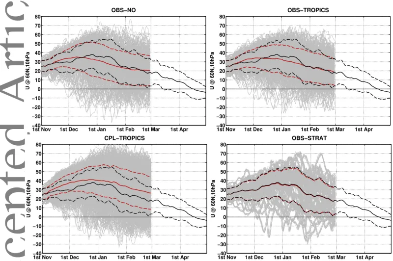
4.1. Interannual variability in the stratospheric polar night jet
As a first step, we analyze how year-to-year variability in the polar stratosphere is represented in the different relaxation experiments, where an emphasis is placed on the tropical relaxation experiments with and without a coupled ocean to investigate the role that air-sea interaction in the extratropics might play in this context. Figure 4 shows the development of the zonal mean zonal wind at 60◦N, 10hPa during winter, representing the strength and variability of the stratospheric polar night jet (PNJ). The climatological strength of the PNJ increases until its peak at the end of December/beginning of January (ERA- Interim mean over all winters; solid black line), and the highest interannual variability can be observed in January (dashed black lines, showing the range of the all-winter-average +- two standard deviations in ERA-Interim). In the atmosphere-only model runs (solid red lines), the PNJ is stronger than observed in early winter, with a maximum that is too early and too weak in mid December.
This leads to an underestimation of the PNJ strength in January, before the modeled PNJ winds follow the reanalysis winds very closely again in February. For this evolution and the described deficiencies, it does not make a big difference if relaxation is applied in the tropics (OBS-TROPICS) or not (OBS-NO). The variability of the PNJ in the model is comparable to the observed variability, only slightly weaker in mid-winter. No obvious effect of tropical relaxation (compared to no relaxation) can be detected.
When no relaxation is applied (OBS-NO), a few positive and negative extremes have a larger amplitude than in OBS-TROPICS.
Interestingly, an effect from coupling the atmosphere and ocean is clearly visible: the PNJ in CPL-TROPICS is stronger than in ERA-Interim and in the tropical relaxation experiments throughout the whole winter. The variability, however, is again comparable to that observed. We suspect that the stronger winds in the PNJ result from the SSTs which are computed interactively in the free-running ocean model in CPL-TROPICS after initialization. A potential bias or drift in the modeled SSTs can have an effect on the overlying troposphere (Keeley et al.
2012) and might also affect the stratosphere. Scaifeet al.(2011) have reported that the common cold bias in the North Atlantic
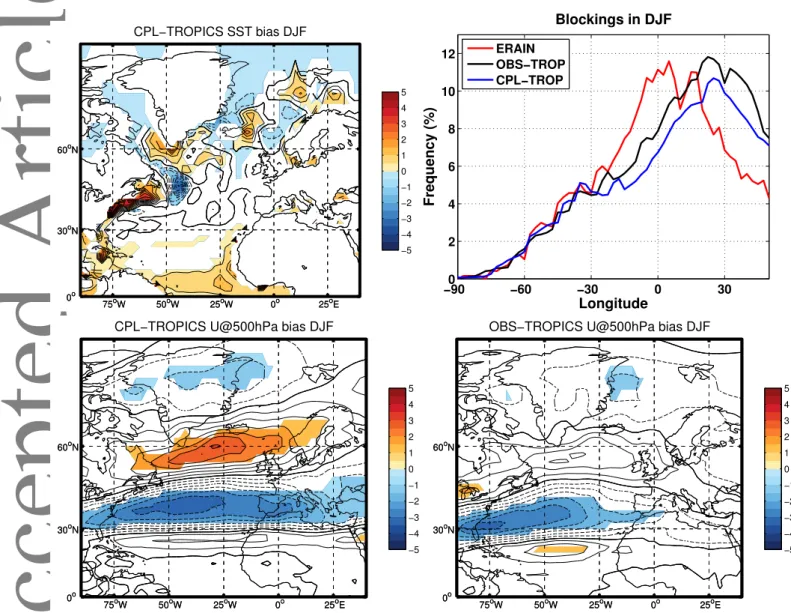
leads to an underestimation of the frequency of tropospheric blockings. Other studies, e.g. as reported by Andrewset al.(1987) and Nishiiet al.(2009), have linked tropospheric blockings to a weakened stratospheric PNJ as the tropospheric blockings can act as wave sources for upward propagating planetary waves in the extratropics. To test if an altered link between SSTs, blockings and the NH winter stratosphere might also be the cause for the stronger PNJ in CPL-TROPICS, we compute the winter mean differences between the modeled SSTs in CPL-TROPICS and observed SSTs.
Although we use forecast experiments in our study, which are initialized every November and then run for only four months, a clear drift of the SSTs towards significantly warmer values off the east coast of the United States and significantly colder values off Newfoundland extending to the southeast can be seen in Figure 5 a). The magnitude of the SST anomalies in Figure 5 a), which exceed 4◦C locally, are comparable to typical values of the North Atlantic cold bias found in coupled models (Wanget al. 2014) as in the Kiel Climate Model (Park et al. 2009) discussed by Drews et al. (2015), where the cold bias reaches up to 10◦C (see also Scaifeet al.2011; Keeleyet al.2012; Jungclauset al.
2013; Wanget al.2014). In Figure 5 a), the maximum cold bias is located further west than is typical, but this might be due to the short simulation time. To investigate whether and how these SST anomalies affect the tropospheric circulation, Figures 5 c) and d) show the mean bias in the zonal wind at 500hPa in DJF in the uncoupled and coupled model experiments using relaxation in the Tropics. The figures reveal a significant overestimation of the westerly winds in a zonal band in the northern North Atlantic, extending over Scandinavia, and a significant underestimation in a zonal band south of that in CPL-TROPICS. This pattern resembles the spatial pattern of a positive NAO phase and is very similar to the coupled model wind bias described in Keeleyet al. (2012), and which Keeley et al.(2012) show is directly attributable to the cold SST bias. In OBS-TROPICS, only the weak bias in the subtropics is significant but is also less pronounced than in CPL-TROPICS. Consistent with that, an effect on tropospheric blockings can be observed (Figure 5 b)). For Figure 5 b) the frequency of blockings in the North Atlantic region in ERA- Interim, OBS-TROPICS and CPL-TROPICS was computed as in Gollan et al. (2015) based on GPH at 500hPa. Aside from
This article is protected by copyright. All rights reserved.
Accepted Article
an eastward shift of the blocking frequency peak over Europe in both relaxation experiments which has been discussed in Gollan et al.(2015) for experiments using relaxation towards ERA40, the blocking frequency is reduced in CPL-TROPICS compared to OBS-TROPICS. Although this can, of course, not serve as a proof, it at least supports the hypothesized link between biased extratropical SSTs, altered tropospheric blocking occurrence and changes in the PNJ strength found for CPL-TROPICS.
As expected and defined by the experimental setup, the evolution and variability of the PNJ winds in OBS-STRAT follow the observations.
4.2. Skill in predicting SSW occurrence
To learn something about the general skill of the different relaxation experiments in terms of predicting extreme weak events in the stratosphere, i.e. SSWs, the time series of SSW risk is shown for each experiment in Figure 6. The SSW risk of one winter season (NDJF) is defined here as the fraction of ensemble members which predict a major SSW at some time during that season. From the resulting time series we use the median (blue line and blue number in each panel of Figure 6) to define if the respective experiment predicted a major SSW in that winter (SSW risk above median in that winter) or not (SSW risk equal to or below median). That means that more than 5 out of the 9 ensemble members need to have a major SSW in one winter in CLIM-NO and OBS-NO to define that these experiments predicted an event in that winter, in CLIM-TROPICS and OBS-TROPICS more than 4 out of 9 ensemble members with an SSW are needed, and more than 8 out of the 28 ensemble members in CPL-TROPICS, as can be seen from Figure 6. By comparing these SSW predictions with the observed SSWs from ERA-Interim, we obtain two characteristic numbers for each experiment, given in black in each panel of Figure 6: (1) the number of correct predictions, which is derived from the number of hits, i.e. winters where an observed SSW has been correctly predicted by the model, and the number of correct rejections, i.e.
winters where the model correctly predicted no SSW, and (2) the number of false predictions, which consists of the number of misses, i.e. where the model did not predict an observed SSW, and the number of false alarms where the model predicted a SSW
although none occurred. The observed SSW frequency obtained from ERA-Interim is given in red in each panel for the period covered by the respective experiment (1981/1982–2013/2014 for CPL-TROPICS, 1979/1980–2013/2014 for all others.) Please note that the number given here (0.4) differs from the widespread 0.5 (“one SSW every second winter”; e.g. Erlebachet al.(1996);
Labitzke and Naujokat (2000); Charltonet al.(2007)) as it refers only to November through February (with March being excluded since March is not covered by the experiments) and as it counts only the number of winters where at least one SSW occurs and not the total number of observed SSWs.
Without any relaxation and with climatological SSTs at the lower boundary (CLIM-NO), the model predicts SSW occurrence in more than 50% of the winters wrong. OBS-NO, CLIM-TROPICS and OBS-TROPICS all show the same skill in terms of percentage of correct (57%) and false (43%) predictions. Comparison of these three experiments tells us that the largest effect comes from tropical SSTs: using observed instead of climatological SSTs (OBS-NO vs. CLIM-NO) already leads to an increase in SSW skill compared to CLIM-NO which is not further increased by adding relaxation in the tropical atmosphere (OBS-TROPICS vs. OBS-NO). CLIM-TROPICS, however, shows the same skill, but assuming that the effect of relaxation overwhelms the effect of SSTs, in this case in the Tropics, and finding no influence from extratropical SSTs here (OBS-TROPICS compared to CLIM-TROPICS) allows us draw this conclusion.
Aside from the experiments using relaxation in the NH stratosphere, from which we would expect perfect SSW forecasts, the CPL-TROPICS experiment appears to be the best one in terms of percentage of correct (70%) and false (30%) predictions.
The median of SSW risk in this experiment is considerably lower than the observed one (0.29 compared to 0.39) which is consistent with the result of the previous section where the PNJ was shown to be stronger than observed, i.e. more difficult to disturb which lowers the likelihood of weak events to occur.
Defining the result of the prediction (correct or false) relative to the median has the effect of removing a bias from the experiment.
The results tell us that by having a perfect forecast of the tropical atmosphere and by allowing two-way atmosphere-ocean interaction in the extratropics, the tendency for SSWs is predicted
This article is protected by copyright. All rights reserved.
Accepted Article
correctly in around 70% of all winter seasons in the ECMWF coupled modelling system used here. The percentage of correct predictions increases to 75% in CPL-TROPICS if we count the
“excuses” for false alarms in two winters where modeled SSWs in February were identified as final warmings in ERA-Interim. It seems that the ECMWF uncoupled model is too prone to having SSWs, consistent with its PNJ being underestimated and hence easier to disturb during most weeks in winter. Although the coupled model version has a bias of opposite sign in the PNJ, which is too strong, this seems to lead to an improvement of SSW risk prediction.
4.3. NAO prediction skill dependence on SSWs
As a last step, we want to build the bridge between the previous sections and investigate the dependance of NAO predictions on the occurrence of SSWs. To do that, we follow and extend the analysis performed by Scaifeet al. (2016) to see if we can confirm their findings with the model used here, and to detect a potential influence from the Tropics or from extratropical atmosphere-ocean coupling. Figure 7 shows the distribution of NAO forecasts for each relaxation experiment, where the red bars include all forecasts of all ensemble members and years, the blue bars include only NAO forecasts of ensemble members which did not predict a SSW, and the green bars include only those forecasts which predicted a SSW. Like in Scaifeet al.(2016), a clear shift of the NAO towards lower values appears in combination with a SSW occurrence. A shift of about the same magnitude but towards more positive NAO values occurs when only predictions without SSWs are considered. As Scaife et al. (2016) point out, this does not prove that the surface NAO is directly driven by the stratosphere, but confirms that the NAO forecast skill depends on the occurrence of events in the stratosphere. We find approximately the same shift in all experiments, independent of any relaxation applied in the Tropics, and independent of SSTs, whether climatological, observed or computed interactively. This also means that the effect of a SSW event on the NAO forecast does not depend on the quality of the SSW predictions which has been shown to differ between the experiments in the previous section.
Finally, we want to address the question of whether the quality of the NAO predictions depends on the prediction of SSWs.
Similar to Figure 2 and Scaifeet al.(2016), we compute the time series of the NAO index three times for each experiment: first averaging for every winter season over all ensemble members (red line in Figure 8), second averaging only over those ensemble members which did not predict a SSW (blue line), and third averaging only over those ensemble members which predicted a SSW some time in that winter (green line). Computing then the correlation between each of these NAO index time series and the observed NAO index from ERA-Interim (black line in Figure 8), says whether or not the NAO forecast skill depends on the prediction of a SSW. Scaifeet al. (2016) found a clear drop of NAO skill to non-significant values when they excluded ensemble members that included a SSW from their NAO forecasts. We also find a drop of NAO prediction skill in some of the experiments;
however, this is not as striking as detected by Scaifeet al.(2016).
A relatively large drop from 0.3 to 0.07 can be found in OBS-NO;
however, this experiment shows no significant NAO skill anyway.
In both atmosphere-only experiments using tropical relaxation, the NAO prediction skill is about the same independent of whether SSWs are included in the prediction or not, although a slight tendency towards better NAO forecasts in predictions without SSWs can be seen. In the coupled model experiment, CPL-TROPICS, the NAO prediction skill is also still significant (0.54 instead of 0.65) when SSWs are excluded. Opposite to the uncoupled tropical relaxation experiments, the NAO prediction skill is higher in CPL-TROPICS when only forecasts which predict a SSW are considered compared to the case where these predictions are excluded, suggesting that a large part of the total skill in this experiment/model version comes from the negative NAO and the ability of the model to correctly predict SSWs.
In summary, we cannot confirm the striking findings of Scaife et al. (2016) that the NAO forecast depends on whether SSWs are included in the forecast or not, although a tendency towards lower (higher) NAO values can be observed when SSWs are (not) included in the forecast. The last point suggests that in the ECMWF model system the NAO forecast skill does not depend strongly on the NAO phase.
This article is protected by copyright. All rights reserved.
Accepted Article
5. Summary and conclusions
In this study, we have investigated the importance of the Tropics, specifying observed sea surface temperature (SST) and sea ice, atmosphere-ocean coupling and the stratosphere for predictions of the NAO. To do that, we have analyzed relaxation experiments with the ECMWF model where different parts of the atmosphere were relaxed towards ERA-Interim to obtain perfect forecasts for these regions. The role of observed SSTs and sea ice has been addressed by prescribing either climatological or observed SST and sea ice at the lower boundary, and by comparing atmosphere- only experiments with coupled atmosphere-ocean simulations.
Our set of seven different experiments has been performed as forecast experiments covering the winters from 1979/80–2013/14, initialized each winter around the beginning of November and run until the end of February. Our results reveal the following:
• Significant prediction skill arises in large parts of the NH when the tropical atmosphere is relaxed towards ERA- Interim, i.e. when the tropical atmosphere is perfectly forecast. Skill increases in some parts of the NH, e.g.
the Greenland-Norwegian Sea, when observed instead of climatological SSTs are used at the lower boundary.
When two-way atmosphere-ocean coupling is allowed in the extratropics, general prediction skill increases further over the North Atlantic and Europe. Relaxation in the NH stratosphere leads to pronounced significant prediction skill over Greenland, Iceland, North America and southern Europe.
• Interannual variability of the NAO is best reproduced when perfect knowledge about the NH stratosphere is available together with perfect knowledge of SST and sea ice. Then, a NAO prediction skill of 0.72 can be achieved during the ERA-Interim period which highlights the importance of the stratosphere for the dynamics in the North Atlantic. Relaxation of the tropical atmosphere together with extratropical atmosphere-ocean coupling can also account for more than 40% of the interannual NAO variability.
• In the atmosphere-only forecast experiments, the strength of the stratospheric polar night jet (PNJ) is slightly
overestimated compared to ERA-Interim in early winter, and underestimated in January, independent of whether relaxation is applied in the Tropics. Using relaxation in the Tropics and allowing atmosphere-ocean interaction in the extratropics, as in the coupled model experiment, leads to an overestimation of the PNJ strength throughout the winter. This might be attributed to a drift in the modeled SSTs which leads to an anomaly pattern resembling the North Atlantic cold bias observed in many models (Wang et al.2014; Drewset al.2015), and to an underestimation of tropospheric blockings in the North Atlantic/Europe sector (Scaifeet al.2011).
• Consistent with the stronger PNJ, the lowest frequency of major stratospheric sudden warmings (SSWs) is found in the coupled model experiment with tropical relaxation.
However, after statistically removing the PNJ bias from this simulation, SSWs are predicted best under these conditions, while the ECMWF atmosphere-only model version seems to be too prone to having SSWs. Comparison with the other experiments reveals that a perfect forecast of the tropical atmosphere and allowing two-way atmosphere- ocean coupling seem to be key ingredients for SSW predictions being successful in 70% of all cases.
• A clear shift of the predicted NAO towards lower values appears in combination with SSW occurrence, confirming the findings of Scaife et al. (2016). Approximately the same shift appears in all experiments which suggests the independence of this result from the quality of SSW prediction.
Unlike Scaife et al.(2016) or Sigmond et al.(2013), only a small reduction of NAO prediction skill could be found when members predicting a SSW are excluded from the NAO forecast.
This suggests a weaker impact of SSWs on NAO predictions in the ECMWF model compared to these other models. Nevertheless, our study was able to highlight the importance of the stratosphere for NAO variability, and to detect some important ingredients for successful predictions of major SSWs.
This article is protected by copyright. All rights reserved.
Accepted Article
Acknowledgements
We are grateful to ECMWF for the provision of the models used here and also for the use of computer facilities to carry out the model runs. Support from the German Ministry for Education and Research (BMBF) through MiKlip2, subproject 01LP1517D (ATMOS-MODINI) is also gratefully acknowledged, as is support from the GEOMAR Helmholtz Centre for Ocean Research Kiel.
This study was also supported by the EC FP7 project SPECS (grant agreement number 308378).
References
Andrews DG, Holton J, Leovy C. 1987. Middle Atmosphere Dynamics.
Academic Press.
Ayarzag¨uena B, Langematz U, Meul S, Oberl¨ander S, Abalichin J, Kubin A.
2013. The role of climate change and ozone recovery for the future timing of Major Stratospheric Warmings.Geophys. Res. Lett.40: 2460–2465, doi:
10.1002/grl.50477.
Baldwin M, Dunkerton T. 2001. Stratospheric harbingers of anomalous Weather Regimes.Science294: 581–584.
Bell CJ, Gray LJ, Charlton-Perez AJ, Joshi MM, Scaife AA. 2009.
Stratospheric Communication of El Nino Teleconnections to European Winter.J. Climate22(15): 4083–4096, doi:10.1175/2009JCLI2717.1.
Boer GJ, Hamilton K. 2008. QBO influence on extratropical predictive skill.
Climate Dyn.31(7-8): 987–1000, doi:10.1007/s00382-008-0379-5.
Broennimann S. 2007. Impact of El Nino Southern Oscillation on European climate. Reviews of Geophysics 45(2): RG3003, doi:
10.1029/2006RG000199.
Broennimann S, Xoplaki E, Casty C, Pauling A, Luterbacher J. 2007. ENSO influence on Europe during the last centuries.Climate Dynamics28(2-3):
181–197, doi:10.1007/s00382-006-0175-z.
Butler AH, Polvani LM, Deser C. 2014. Separating the stratospheric and tropospheric pathways of El Nino-Southern Oscillation teleconnec- tions.Environmental Research Letters9(2): 024 014, doi:10.1088/1748- 9326/9/2/024014.
Cassou C. 2008. Intraseasonal interaction between the Madden-Julian Oscillation and the North Atlantic Oscillation.Nature455(7212): 523–527, doi:10.1038/nature07286.
Charlton AJ, Polvani LM, Perlwitz J, Sassi F, Manzini E, Shibata K, Pawson S, Nielsen JE, Rind D. 2007. A new look at stratospheric sudden warmings.
Part II: Evaluation of numerical model simulations.J. Climate20(3): 470–
488, doi:10.1175/JCLI3994.1.
Cohen J, Entekhabi D. 1999. Eurasian snow cover variability and Northern Hemisphere climate predictability.Geophysical Research Letters26(3):
345–348, doi:10.1029/1998GL900321.
Dee DP, Uppala SM, Simmons AJ, Berrisford P, Poli P, Kobayashi S, Andrae U, Balmaseda MA, Balsamo G, Bauer P, Bechtold P, Beljaars ACM, van de Berg L, Bidlot J, Bormann N, Delsol C, Dragani R, Fuentes M, Geer AJ, Haimberger L, Healy SB, Hersbach H, H´olm EV, Isaksen L, K˚allberg P, K¨ohler M, Matricardi M, McNally AP, Monge-Sanz BM, Morcrette JJ, Park BK, Peubey C, de Rosnay P, Tavolato C, Th´epaut JN, Vitart F.
2011. The ERA-Interim reanalysis: configuration and performance of the data assimilation system.Q.J.R. Meteorol. Soc.137(656): 553–597, URL http://dx.doi.org/10.1002/qj.828.
Douville H. 2009. Stratospheric polar vortex influence on Northern Hemisphere winter climate variability.Geophysical Research Letters36:
L18 703, doi:10.1029/2009GL039334.
Drews A, Greatbatch RJ, Ding H, Latif M, Park W. 2015. The use of a flow field correction technique for alleviating the North Atlantic cold bias with application to the Kiel Climate Model.Ocean Dynamics65(8): 1079–1093, doi:10.1007/s10236-015-0853-7.
Erlebach P, Langematz U, Pawson S. 1996. Simulations of stratospheric sudden warmings in the Berlin troposphere stratosphere mesosphere GCM.
Ann. Geophys.14(4): 443–463, doi:10.1007/s00585-996-0443-6.
Fereday DR, Maidens A, Arribas A, Scaife AA, Knight JR. 2012. Seasonal forecasts of northern hemisphere winter 2009/10.Environmental Research Letters7(3): 034 031, doi:10.1088/1748-9326/7/3/034031.
Fraedrich K, Muller K. 1992. Climate Anomalies In Europe Associated With ENSO Extremes.International Journal of Climatology12(1): 25–31, doi:
10.1002/joc.3370120104.
Gollan G, Greatbatch RJ. 2015. On the Extratropical Influence of Variations of the Upper-Tropospheric Equatorial Zonal-Mean Zonal Wind during Boreal Winter.Journal of Climate28(1): 168–185, doi:10.1175/JCLI-D- 14-00185.1.
Gollan G, Greatbatch RJ, Jung T. 2015. Origin of variability in Northern Hemisphere winter blocking on interannual to decadal timescales.Geophys.
Res. Lett.42(22): 10,037–10,046, doi:10.1002/2015GL066572.
Greatbatch RJ. 2000. The North Atlantic Oscillation. Stochastic Envi- ronmental Research and Risk Assessment 14(4-5): 213–242, doi:
10.1007/s004770000047.
Greatbatch RJ, Gollan G, Jung T, Kunz T. 2012. Factors influencing Northern Hemisphere winter mean atmospheric circulation anomalies during the period 1960/61 to 2001/02.Quarterly Journal of the Royal Meteorological Society138(669): 1970–1982, doi:10.1002/qj.1947.
Greatbatch RJ, Gollan G, Jung T, Kunz T. 2015. Tropical origin of the severe European winter of 1962/1963.Quarterly Journal of the Royal Meteorological Society141(686): 153–165, doi:10.1002/qj.2346.
Greatbatch RJ, Jung T. 2007. Local versus tropical diabatic heating and the winter North Atlantic Oscillation.Journal of Climate20(10): 2058–2075, doi:10.1175/JCLI4125.1.
Greatbatch RJ, Lu J, Peterson KA. 2004. Nonstationary impact of ENSO on Euro-Atlantic winter climate. Geophysical Research Letters 31(2):
This article is protected by copyright. All rights reserved.
Accepted Article
L02 208, doi:10.1029/2003GL018542.
Hoerling MP, Hurrell JW, Xu TY. 2001. Tropical origins for recent North Atlantic climate change. Science 292(5514): 90–92, doi:
10.1126/science.1058582.
Holton JR, Tan HC. 1980. The influence of the equatorial quasi-biennial oscillation on the global circulation at 50 mb.J. Atmos. Sci.37: 2200–2208.
Holton JR, Tan HC. 1982. The quasi-biennial oscillation in the Northern Hemisphere lower stratosphere.J. Meteor. Soc. Japan60: 140–148.
Hoskins B, Fonseca R, Blackburn M, Jung T. 2012. Relaxing the Tropics to an ’observed’ state: analysis using a simple baroclinic model.Quarterly Journal of the Royal Meteorological Society138(667): 1618–1626, doi:
10.1002/qj.1881.
Huang JP, Higuchi K, Shabbar A. 1998. The relationship between the North Atlantic Oscillation and El Nino Southern Oscillation.Geophysical Research Letters25(14): 2707–2710, doi:10.1029/98GL01936.
Huntingford C, Marsh T, Scaife AA, Kendon EJ, Hannaford J, Kay AL, Lockwood M, Prudhomme C, Reynard NS, Parry S, Lowe JA, Screen JA, Ward HC, Roberts M, Stott PA, Bell VA, Bailey M, Jenkins A, Legg T, Otto FEL, Massey N, Schaller N, Slingo J, Allen MR. 2014. Potential influences on the United Kingdom’s floods of winter 2013/14.Nature Climate Change 4(9): 769–777, doi:10.1038/NCLIMATE2314.
Hurrell JW. 1995. Decadal Trends In the North-Atlantic Oscillation - Regional Temperatures and Precipitation.Science269(5224): 676–679, doi:
10.1126/science.269.5224.676.
Hurrell JW. 1996. Influence of variations in extratropical wintertime teleconnections on Northern Hemisphere temperature. Geophysical Research Letters23(6): 665–668, doi:10.1029/96GL00459.
Hurrell JW, Kushnir Y, Ottersen G, Visbeck M. 2003. An Overview of the North Atlantic Oscillation. In:The North Atlantic Oscillation: Climatic Significance and Environmental Impact, American Geophysical Union, pp.
1–35.
Ineson S, Scaife AA. 2009. The role of the stratosphere in the European climate response to El Nino. Nature Geoscience 2(1): 32–36, doi:
10.1038/NGEO381.
Jung T, Miller MJ, Palmer TN. 2010a. Diagnosing the Origin of Extended- Range Forecast Errors.Monthly Weather Review138(6): 2434–2446, doi:
10.1175/2010MWR3255.1.
Jung T, Palmer TN, Rodwell MJ, Serrar S. 2010b. Understanding the Anomalously Cold European Winter of 2005/06 Using Relax- ation Experiments. Monthly Weather Review 138(8): 3157–3174, doi:
10.1175/2010MWR3258.1.
Jung T, Vitart F, Ferranti L, Morcrette JJ. 2011. Origin and predictability of the extreme negative NAO winter of 2009/10.Geophysical Research Letters38:
L07 701, doi:10.1029/2011GL046786.
Jungclaus JH, Fischer N, Haak H, Lohmann K, Marotzke J, Matei D, Mikolajewicz U, Notz D, von Storch JS. 2013. Characteristics of the ocean simulations in the Max Planck Institute Ocean Model (MPIOM) the
ocean component of the MPI-Earth system model.Journal of Advances In Modeling Earth Systems5(2): 422–446, doi:10.1002/jame.20023.
Keeley SPE, Sutton RT, Shaffrey LC. 2012. The impact of North Atlantic sea surface temperature errors on the simulation of North Atlantic European region climate. Quarterly Journal of the Royal Meteorological Society 138(668): 1774–1783, doi:10.1002/qj.1912.
Labitzke K, Naujokat B. 2000. The lower Arctic stratosphere in winter since 1952.SPARC Newsletter15: 11–14.
Lin H, Brunet G, Derome J. 2009. An Observed Connection between the North Atlantic Oscillation and the Madden-Julian Oscillation.Journal of Climate 22(2): 364–380, doi:10.1175/2008JCLI2515.1.
Lin H, Brunet G, Yu B. 2015. Interannual variability of the Madden- Julian Oscillation and its impact on the North Atlantic Oscillation in the boreal winter. Geophys. Res. Lett. : 2015GL064 547–URL http://dx.doi.org/10.1002/2015GL064547.
Maidens A, Arribas A, Scaife AA, MacLachlan C, Peterson D, Knight J.
2013. The Influence of Surface Forcings on Prediction of the North Atlantic Oscillation Regime of Winter 2010/11.Monthly Weather Review141(11):
3801–3813, doi:10.1175/MWR-D-13-00033.1.
Manzini E, Giorgetta MA, Esch M, Kornblueh L, Roeckner E. 2006. The influence of sea surface temperatures on the northern winter stratosphere:
Ensemble simulations with the MAECHAM5 model.J. Climate19(16):
3863–3881, doi:10.1175/JCLI3826.1.
Marshall AG, Scaife AA, Ineson S. 2009. Enhanced Seasonal Prediction of European Winter Warming following Volcanic Eruptions.Journal of Climate22(23): 6168–6180, doi:10.1175/2009JCLI3145.1.
Mitchell DM, Gray LJ, Anstey J, Baldwin MP, Charlton-Perez AJ. 2013.
The Influence of Stratospheric Vortex Displacements and Splits on Surface Climate.J. Climate26(8): 2668–2682, doi:10.1175/JCLI-D-12-00030.1.
Murphy JM. 1990. Assessment of the Practical Utility of Extended Range Ensemble Forecasts.Quarterly Journal of the Royal Meteorological Society 116(491): 89–125.
Nishii K, Nakamura H, Miyasaka T. 2009. Modulations in the planetary wave field induced by upward-propagating Rossby wave packets prior to stratospheric sudden warming events: A case-study.Quarterly Journal of the Royal Meteorological Society135(638): 39–52, doi:10.1002/qj.359.
Park W, Keenlyside N, Latif M, Stroeh A, Redler R, Roeckner E, Madec G. 2009. Tropical Pacific Climate and Its Response to Global Warming in the Kiel Climate Model. Journal of Climate 22(1): 71–92, doi:
10.1175/2008JCLI2261.1.
Pascoe CL, Gray LJ, Scaife AA. 2006. A GCM study of the influence of equa- torial winds on the timing of sudden stratospheric warmings.Geophysical Research Letters33(6): L06 825, doi:10.1029/2005GL024715.
Quiroz RS. 1977. Tropospheric-stratospheric Polar Vortex Breakdown of January 1977. Geophys. Res. Lett. 4(4): 151–154, doi:
10.1029/GL004i004p00151.
This article is protected by copyright. All rights reserved.
Accepted Article
Ratcliffe RAS, Murray R. 1970. New Lag Associations Between North Atlantic Sea Temperature and European Pressure Applied To Long-range Weather Forecasting. Quarterly Journal of the Royal Meteorological Society96(408): 226–&, doi:10.1002/qj.49709640806.
Rodwell MJ, Folland CK. 2002. Atlantic air-sea interaction and seasonal predictability. Quarterly Journal of the Royal Meteorological Society 128(583): 1413–1443, doi:10.1256/00359000260247291.
Scaife AA, Arribas A, Blockley E, Brookshaw A, Clark RT, Dunstone N, Eade R, Fereday D, Folland CK, Gordon M, Hermanson L, Knight JR, Lea DJ, MacLachlan C, Maidens A, Martin M, Peterson AK, Smith D, Vellinga M, Wallace E, Waters J, Williams A. 2014. Skillful long-range prediction of European and North American winters.Geophysical Research Letters 41(7): 2514–2519, doi:10.1002/2014GL059637.
Scaife AA, Copsey D, Gordon C, Harris C, Hinton T, Keeley S, O’Neill A, Roberts M, Williams K. 2011. Improved Atlantic winter blocking in a climate model. Geophysical Research Letters 38: L23 703, doi:
10.1029/2011GL049573.
Scaife AA, Karpechko AY, Baldwin MP, Brookshaw A, Butler AH, Eade R, Gordon M, MacLachlan C, Martin N, Dunstone N, Smith D. 2016. Seasonal winter forecasts and the stratosphere.Atmosph. Sci. Lett.17: 51–56, doi:doi:
10.1002/asl.598.
Scaife AA, Knight JR. 2008. Ensemble simulations of the cold European winter of 2005-2006. Quarterly Journal of the Royal Meteorological Society134(636): 1647–1659, doi:10.1002/qj.312.
Scaife AA, Knight JR, Vallis GK, Folland CK. 2005. A stratospheric influence on the winter NAO and North Atlantic surface climate. Geophysical Research Letters32(18): L18 715, doi:10.1029/2005GL023226.
Sigmond M, Scinocca JF, Kharin VV, Shepherd TG. 2013. Enhanced seasonal forecast skill following stratospheric sudden warmings.Nature Geoscience 6(2): 98–102, doi:10.1038/NGEO1698.
Stenchikov G, Hamilton K, Robock A, Ramaswamy V, Schwarzkopf MD.
2004. Arctic oscillation response to the 1991 Pinatubo eruption in the SKYHI general circulation model with a realistic quasi-biennial oscillation.
Journal of Geophysical Research-atmospheres 109(D3): D03 112, doi:
10.1029/2003JD003699.
Stockdale TN, Molteni F, Ferranti L. 2015. Atmospheric initial conditions and the predictability of the Arctic Oscillation.Geophysical Research Letters 42(4): 1173–1179, doi:10.1002/2014GL062681.
Taws SL, Marsh R, Wells NC, Hirschi J. 2011. Re-emerging ocean temperature anomalies in late-2010 associated with a repeat negative NAO.Geophysical Research Letters38: L20 601, doi:10.1029/2011GL048978.
Thompson DWJ, Baldwin MP, Wallace JM. 2002. Stratospheric connection to Northern Hemisphere wintertime weather: Implications for prediction. J. Climate 15(12): 1421–1428, doi:10.1175/1520- 0442(2002)015¡1421:SCTNHW¿2.0.CO;2.
Toniazzo T, Scaife AA. 2006. The influence of ENSO on winter North Atlantic climate. Geophysical Research Letters 33(24): L24 704, doi:
10.1029/2006GL027881.
Trenberth KE, Branstator GW, Karoly D, Kumar A, Lau NC, Ropelewski C. 1998. Progress during TOGA in understanding and modeling global teleconnections associated with tropical sea surface temperatures.
Journal of Geophysical Research-oceans 103(C7): 14 291–14 324, doi:
10.1029/97JC01444.
Wang C, Zhang L, Lee SK, Wu L, Mechoso CR. 2014. A global perspective on CMIP5 climate model biases.Nature Climate Change4(3): 201–205, doi:10.1038/NCLIMATE2118.
Watson PAG, Weisheimer A, Knight JR, Palmer TN. 2016. The role of the tropical West Pacific in the extreme northern hemisphere winter of 2013/14.
J. Geophys. Res.-Atmos.doi:10.1002/2015JD024048.
Wu Q, Zhang X. 2010. Observed forcing-feedback processes between Northern Hemisphere atmospheric circulation and Arctic sea ice coverage.
Journal of Geophysical Research-atmospheres 115: D14 119, doi:
10.1029/2009JD013574.