Meson spectroscopy in Large-N QCD Dissertation

(1)

Meson spectroscopy in Large-N QCD

Dissertation

zur Erlangung des Doktorgrades der Naturwissenschaften (Dr. rer. nat.) der Fakultät für Physik

der Universität Regensburg

vorgelegt von

Luca Castagnini

aus Ivrea, Italien

May 2015

(2)

Promotionsgesuch eingereicht an: 27.01.2015

Die Promotionsarbeit wurde angeleitet von Prof. Dr. Gunnar Bali.

Das Promotionskolloquium fand am 23.06.2015 statt.

Prüfungsausschuss:

Vorsitzender Prof. Dr. Christian Schüller 1. Gutachter Prof. Dr. Gunnar Bali 2. Gutachter Prof. Dr. Meinulf Göckeler weiterer Prof. Dr. Milena Grifoni

(3)

Introduction 1

Quantum Chromodynamics (QCD) is the commonly accepted theory of strong interactions. It is formulated in terms of elementary fields (quarks and gluons), whose interactions obey the principles of a relativistic quantum field theory, with a non-abelian gauge invariance based on theSU(3)group. It is described in the continuum Minkowski space by the Lagrangian:

L= ¯ψ_qⁱ iγ^µD_µ^ij−m_qδ^ij

ψ^j_q− 1

4F_µν^a F^aµν (1.1)

whereψ_qⁱ denotes the quark field with colour indexi= 1, . . . ,3andD^ijµ is the covariant derivative:

Dîj_µ =δîj∂_µ+ig_sAâ_µtâ,ij (1.2) Aµis the gauge (gluon) field,gs is the coupling constant while the traceless Hermitian matricestâ (fora = 1, . . . ,8)are the generators of the Lie algebrasu(3)with the nor- malizationTr (tât^b) = δâb/2and[tâ, t^b] = i fâbct^c. Lastly,F_µνâ is the non-Abelian field strength defined as

F_µνâ =∂µAâ_ν −∂νAâ_µ+gsf_abcA^b_µA^c_ν (1.3) The theory is characterised by gauge invariance, i.e. given an element of thesu(N) algebraω(x)the theory is invariant under the local transformation,

ψ(x) →ψ⁰(x) = ω(x)ψ(x) (1.4)

ψ(x)¯ →ψ¯⁰(x) = ψ(x)ω¯ ⁻¹(x)

A_µ(x) →A⁰_µ(x) = ω(x)A_µ(x)ω⁻¹(x) + i

g_s(∂_µω(x))ω⁻¹(x)

(6)

1. Introduction

Non-abelian gauge theories behave in a peculiar way: the interactions weaken at short distances, or, equivalently, large momentum transfers. This is due to the running of the coupling constantg_s²which becomes smaller than 1 for energies larger than 1 GeV. In this regime, and for even larger energies such as in high energy proton-proton collisions, the coupling constant is small and the perturbative approach becomes a reli- able tool. At low energies, however, the running coupling becomes large; in this regime many features of QCD are determined by non-perturbative phenomena, like confinement and chiral symmetry breaking. For this reason, the theoretical derivation of low energy QCD properties must rely on non-perturbative methods.

The standard non-perturbative definition of QCD is based on lattice regularisation [1], which makes the theory mathematically well-defined and amenable to analytical as well as to numerical studies. Thanks to theoretical, algorithmic and computer-power progress, during the last decade many large-scale dynamical lattice QCD (LQCD) computations have been performed at realistic values of the physical parameters, allowing one to obtain numerical predictions in energy regimes otherwise inaccessible. Although brute forcebrings evidence that the QCD is indeed the correct theory of strong interactions, numerical results may not provide an analytical understanding of the theory.

A different approach to QCD was suggested by Gerard ’t Hooft in [2] which consists of studying anSU(N)based QCD, where the number of coloursN is taken to infinity and the couplinggis sent to zero, keeping the product g²N, as well as the number of flavournf, fixed. In this limit one finds that the amplitudes for physical processes are determined by a particular subset of (planar) Feynman diagrams, while other diagrams are suppressed by powers of1/N. Due to these mathematical simplifications, the low- energy spectrum consists of stable meson and glueball states, and the scattering matrix becomes trivial. Ideally one would then study the physical N = 3 case expanding around the1/N → 0limit, however the ’t Hooft limit has proven so far to be still too complicated to be solved analytically.

Another non-perturbative approach to low-energy properties of strongly coupled non-Abelian gauge theories is based on the conjectured correspondence between gauge and string theories [3–5]. During the last decade, many studies have employed techniques based on this correspondence, to build models which reproduce (at least qual- itatively) the main features of the mesonic spectrum of QCD. Remarkably, the large-N limit plays a technically crucial role also in the context of these holographic computations: the correspondence relates the strongly coupled regime of a gauge theory with an infinite number of colors to the classical gravity limit of a dual string model in an anti-de Sitter spacetime, a setup that can be studied with analytical or semi-analytical methods.

In order to understand whether predictions derived from approaches relying on the large-N limit can be relevant for the physical case of QCD withN = 3colors, it is crucial to estimate the quantitative impact of finite-N corrections. For this reason, several lattice studies have recently investigated the dependence onN of various quantities of

(7)

1. Introduction

interest—including, for example, string tensions [6–8], the glueball spectrum [9, 10] or the finite-temperature equation of state [11–14]—in differentSU(N)Yang-Mills theories (see [15] for a recent review on largeNlattice results). These works revealed precocious scaling to the large-Nlimit: up to modestO(N⁻²)corrections even theSU(3)andSU(2) theories appear to be “close” to the large-N limit.

The purpose of the present work is to further expand this line of research: by studying with numerical simulations the light mesons in gauge theories based on different SU(N)groups, we extract the dependence on the number of colors. In the past, only the pion and rho meson masses were studied in the largeN limit [16–20]; while most of these works report a rho mass close to the real-world QCD, the authors of [20] found a rho mass which is approximately twice as large. To clarify this discrepancy, we ex- tend the analysis by going to lighter quark masses, larger N, larger volumes and by increasing the statistics and the number of interpolators used to create a meson state.

Part of this work has been published in [21–23]. The results presented here include important improvements, namely the continuum limit extrapolation of the meson spectrum and the computation of non-perturbative large-Nrenormalization constants. This allow us to further restrict our systematic errors and to predict further quantities like the chiral condensate.

In chapter 2 we show how the large-N counting rules associated with the ’t Hooft limit of QCD entail many phenomenological implications, providing intuitive explana- tions for poorly understood features of the real-world theory withN = 3color charges.

Lattice QCD is then formulated in chapter 3 where we explain in detail the methods used in this work. In chapters 4 and 5 we show the results of our simulations, first fo- cusing for each particle mass on its dependence on the quark mass, then presenting the large-N meson spectrum with a discussion on systematic errors and continuum limit extrapolation. We conclude with a comparison between our results and those of other large-N approaches in chapter 6.

(8)

Phenomenology of large-N 2 QCD

2.1. A simple example, the φ

⁴

theory

In order to easily understand the simplifications occurring in the largeN limit, we first examine theO(N)version of the toy-modelφ⁴theory, described by the Lagrangian,

L= 1

2∂µφa∂^µφa−1

2m²φaφa−1

8g²(φaφa)² (2.1) where we have N scalar fields φa (a = 1, . . . , N) and the sum over the repeated a- indexes is implied. In the standard perturbation theory approach, one would choose a regime where the coupling is small, evaluate the contribution of the leading Feynman diagrams and study the quantities as an expansion ofg². In fig. 2.1 we show the first diagrams up tog⁴of a2→2scattering amplitude.

For fixed initial and final fieldsφaandφb, the central diagram in fig. 2.1 will appear N times more often than the other two, due to the extra free choice in the loop index c. If one studies the theory in a particular limit whereN is taken to infinity and g² to zero, while keeping the product λ = g²N finite, the diagram in fig. 2.1-c become 1/N suppressed with respect to the first two diagrams, so that in the large-N limit it can simply be ignored. A similar approach can be employed for QCD whereg² is the running coupling,Nis the number of colours andλis commonly known as the ’t Hooft parameter. In the case of QCD, as we show below, the theory becomes much simpler and only a special class of diagrams survives, however large-N QCD is far from trivial and has not been analytically solved yet.

(9)

2. Phenomenology of large-N QCD

a a

b b

g² = _N^λ a)

c

c a

a

b b

g⁴N = ^λ_N² b)

a b

a a

b b

g⁴= _N^λ²2

c)

Figure 2.1.: Three possibleO(g²)Feynman diagrams for a given couple of input/output fieldsφaandφb. The diagram in the center occursN times, due to the free indexc.

2.2. The double-line notation

Although large-N QCD is far from been analytically solved, one can say a lot about its phenomenology just by studying the type of diagrams that survive. In order to simplify the discussion, we rescale the gluon and fermion fields as,

Aµ→ 1

gAµ, ; ψ→√

N ψ ; 6D→γµ(1∂^µ+iA^µ) (2.2) so that the Lagrangian of one flavour QCD reads,

L=N

− 1

4λF_µν^a F_µν^a + ¯ψ(i6D−m)ψ

(2.3) where the ’t Hooft parameterλ=g²N assumes the role of the coupling. Since the gluon fields carry two colour indexes, counting powers ofN might become confusing in very complicated diagrams. One way to solve this problem is introducing the double-line notation, which is, one draws graphs with one line per colour index rather than per particle. In a gluon-fermion vertex (see fig. 2.2), the gluon is thus replaced by two lines that are attached to the single fermion line with which they interact.

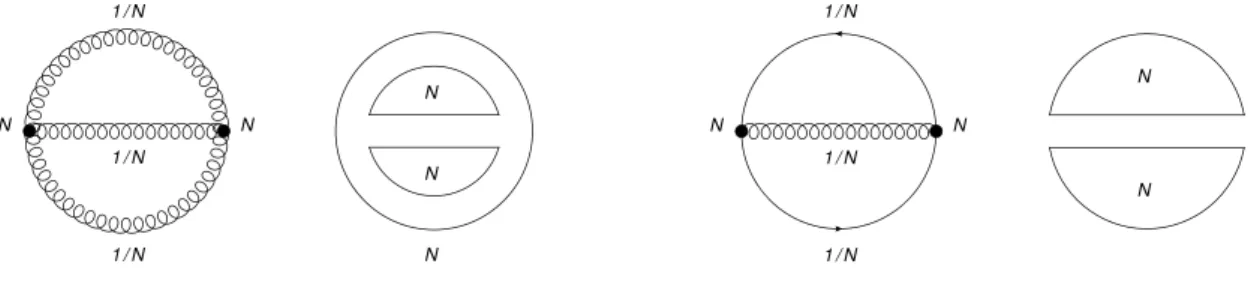
In order to establish which diagrams survive and which ones are suppressed, we need to count the powers ofN associated to them. For any complicated diagram, each vertex carries a factorN due to the coupling and for each propagator we have a factor 1/N. With the double line notation, we can easily count the closed colour loops, to each of which a factorN is associated, due to the free choice of the internal colour index (see figs. 2.3-2.4). Let us examine a generic vacuum diagram, i.e. a diagram with no external legs, like those of fig 2.3. We can think of such a diagram as a surface made of polygons,

(10)

a a b

b

Figure 2.2.: Double line notation for a fermions-gluon vertex. The gluon carries two color indexes.

which correspond to the colour loops, whose edges (E) and vertexes (V) cut the surface into many faces (F). The totalN factor carried by such a diagram will thus be:

N^F^+V^−E =N^χ. (2.4)

χis the well known Euler characteristic, it is a topological invariant and does not de- pend on the way we cut the surface.

1 / N 1 / N 1 / N

N N

N N N

1 / N 1 / N 1 / N

N N

Figure 2.3.: Double line notation for a gluonic (left) and fermionic (right) excitation of the vacuum. The former is proportional toN² while the latter toN.

Generally any complicated surface can be thought as a sphere with some handles (H) and some holes (or boundaries, B) and its characteristic reads,

χ= 2−2H−B. (2.5)

It is then clear that the maximum value ofχ is 2, corresponding to a sphere, and the leading diagrams in the large-N limit will be those∝N², or, which is equivalent, those diagrams that can be drawn on the surface of a sphere without intersection of the lines (planar diagrams). In figs. 2.3 and 2.4 one can see how a fermionic loop correspond to a hole in the surface, i.e. one face is missing (B = 1) with respect to a gluon loop.

This is particularly important, it means that any insertion of a fermionic loop in a given

(11)

N N

N

1 / N

1 / N 1 / N

N 1 / N

1 / N

1 / N N

N N N

N N

N

1 / N

1 / N 1 / N

N 1 / N

1 / N

1 / N N

N N

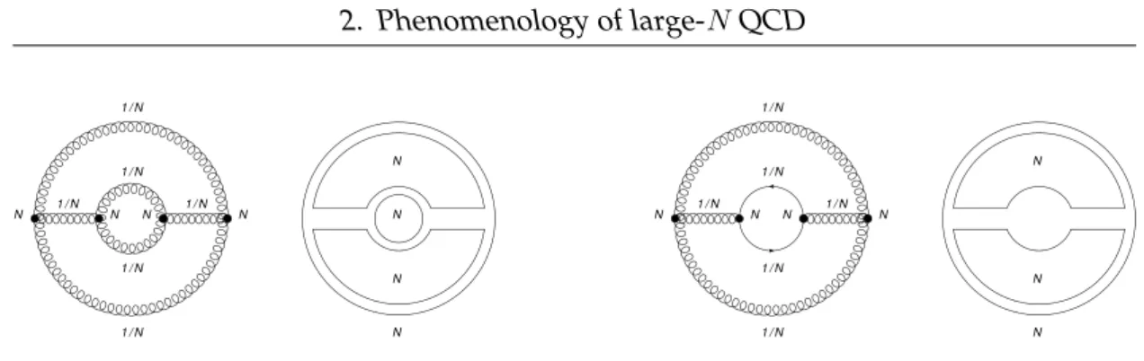
Figure 2.4.: One loop correction to a vacuum diagram. The insertion of a fermion loop (right) is1/N suppressed with respect to a pure gluonic loop (left).

diagram is suppressed by a factor1/N. In other words, the large-N QCD is a theory where all internal quark loops can be ignored as long as the number of flavourn_f is kept fixed, or, in lattice terms, the theory is quenched. One can still analyse diagrams with fermionic lines (for instance, when studying mesons) but they will be present only at the external boundaries.

2.3. Mesons and glueballs

So far we described only vacuum diagrams, however all the considerations hold when we study mesons and glueballs. The diagrams involved are similar to the leading vacuum-to-vacuum diagrams of fig. 2.3, where the glueball and meson operators appear as insertions on the external lines. In particular the leading diagrams for pure gluonic processes are constructed from gluonic vacuum-to-vacuum diagrams and carry a N² factor, while processes involving quarks will be constructed from the leading fermionic vacuum-to-vacuum diagrams, which carry a factorN.

In order to describe the behaviour of mesons and glueballs, we first introduce a generating functionalZJ, which depends on the QCD LagrangianL=NL˜given in eq. (2.1) and on operatorsO_awhich create the desired states,

Z_J = Z

DADψDψexp

iN Z

d⁴x

L˜[A, ψ, ψ] + JO

. (2.6)

We can construct a generic correlator by the use of functional derivatives, hO₁. . . O_ni= (iN)⁻ⁿ δ

δJ1

. . . δ δJn

lnZ_J

J=0

, (2.7)

whereOi = O(xi) andJi = J(xi). For example an n-points function of pure gluonic operatorsGiwill go as,

hG₁. . . G_ni ∝N²⁻ⁿ (2.8)

(12)

As a consequence, in the ’t Hooft limit glueballs are stable objects and processes that involve a glueball decaying into other glueballs or mesons are suppressed.

Mesons are states usually created on the vacuum by bilinear operators Bi = ¯ψΓiψ, however these operators are ill-defined, since the leading fermionic vacuum diagrams are only∝N, so that in the large-N limit a two-point function would be,

hB₁B₂i ∝N¹⁻²⁼⁻¹ −−−−→

N→∞ 0. (2.9)

To avoid this problem, we use the operatorB˜i =√

N Biand then-point meson correlators become,

hB˜1. . .B˜ni ∝N^(2−n)/2 (2.10) which means that interactions between 3 or more mesons are suppressed by powers of 1/√

N. A similar conclusion could be drawn from correlators of mesons and glueballs, thus we can say that in theN → ∞limit QCD consists of stable non-interacting mesons and glueballs, while at large (but finite)N-values QCD is a theory of weekly interacting hadrons.

Another interesting phenomenological property of the ’t Hooft limit is that the Okubo, Zweig and Iizuka (OZI) rule becomes exact when N → ∞. This rule states that processes associated to diagrams which can be divided into two sets of quark lines by cutting only gluon lines are suppressed. These processes involve the annihilation and creation of quarks, thus at least two quark loops must be involved and the amplitude obtains an extra1/N factor with respect to processes which have only one quark loop (see fig. 2.5).

N N N N N

Figure 2.5.: OZI rule. The diagram at the left goes into a stage where only gluon appear and is suppressed by a factor1/N.

2.4. Baryons

Baryons are colourless observables (i.e. they are in a completely antisymmetrised color state) made ofN quarks,

i1,...,iNqⁱ¹. . . qⁱ^N. (2.11)

(13)

For this reason, diagrams involve a number of lines increasing withN and drawing them becomes impossible in the ’t Hooft limit. Nonetheless, one can derive a few scaling laws, as initially indicated by Witten in [24]. One can imagine to split a generic baryon diagram into two parts, one made ofninteracting quark lines and one ofN−n freely propagating quarks (fig. 2.6). The part withninteracting quarks can be thought

} n

Figure 2.6.: A baryon interaction with ann-lines connected component.

of as the result of breaking opennquark lines into a vacuum-to-vacuum graph, which is proportional toN. Since the baryon must be in a total antisymmetric color state, each of thenlines must carry a different color, i.e. for each quark cut we loose a sum over color and thus a genericn-body diagram will be of orderN¹⁻ⁿ. Nonetheless, there are O(Nⁿ) ways to choose n quarks from a N-quark baryon, so that the net effect of an n-body interaction is of orderN. We can think that the total energy of a baryon receives contributions from the mass of the constituent quarks, their kinetic energies and from the quark interactions, all of which scale asO(N)too. Baryons in the large-N limit thus become infinitely heavy objects and the usual way to study them is to treat them as non-relativistic bound states of weakly interacting quarks¹. In this approximation each quark moves independently in a common background potential resulting from the interaction with all the other quarks in the baryon (see [25, 26]) and it can be shown that baryon-baryon scattering is ofO(N)while baryon-meson scattering is ofO(1).

More refined models [27, 28] result in a prediction on the masses of baryons of different spinJ which should match those described in terms of a rotor spectrum,

M =c1N+c2

J(J + 1)

N . (2.12)

This has been recently verified on the lattice in [29] forN = 3,5,7.

1Unfortunately, an elegant relativistic formalism has not yet been found or developed.

(14)

QCD on the lattice 3

3.1. Introduction to lattice QCD

The lattice is a mathematical tool that provides a natural cut-off (the lattice spacing) to remove the ultraviolet infinities that we get in quantum field theory. Physical quantities can be extracted from the lattice only in the continuum limit, where the lattice spacing is taken to zero. By virtue of asymptotic freedom, this can be done easily in lattice simulations, as the coupling constant is an input parameter, and we can force it to take smaller and smaller values, corresponding to a finer and finer lattice spacing. Even if we cannot directly set the coupling constant to zero we can make a fit and extrapolate the physical quantities to their continuum limits.

The lattice formulation emphasizes the close connection between field theory and statistical mechanics and makes it possible to use statistical simulation methods, usually called Monte Carlo programs, to “measure” physical quantities. In this chapter we discuss how to formulate QCD on the lattice, while in the next one we discuss our simulations.

3.2. The connection between quantum field theory and statistical mechanics

In a quantum field theory the Feynmann path integral formulation makes it possible to define a “generating functionalZ” as:

Z[J] = Z

Dφ eⁱ^R^dt^R^d³^{xL(φ)+J φ} (3.1)

(15)

3. QCD on the lattice

The standard way to obtain n-point Green functions of the theory is by differentiating logZ[J]with respect toJ, as already done in eq. (2.7). If we imagine theZ function as a “sum” over every configuration of the fieldφ, we immediately recognise the analogy to the usual expression of the partition function of the canonical ensemble:

Z =X

{φ}

e^−βH[φ], (3.2)

the only difference being that here we have a real weight in the exponential, while above we had an oscillatory term. We can bridge this difference with an analytic con- tinuation of the QFTZfunction to imaginary values of the time. This is the well known

“Wick rotation” (x₀ → ix₄) that leads to the Euclidean form of the actionS_E and theZ function becomes:

Z[J] = Z

Dφe^−S^E^[φ]+^R^d⁴^xJ(x)φ(x) (3.3) Introducing a discrete spacetime (the lattice), made ofN_µnodes separated by a lattice spacing “a” in each directionµ, it is possible to map consistently quantum field theory and statistical field theory with the use of the following identifications:

QFT Statistical Mechanics

Functional integral:R

Dφ Partition functionP

conf

Euclidean action Hamiltonian

Energy of the vacuum Free energy

Green functionsh0|T[O1...On]|0i Correlators:hO1...Oni

MassM Correlation lengthξ = 1/M

Regularization cut-off :Λ inverse lattice spacinga⁻¹ Renormalization:Λ→ ∞ Continuum limit:a→0 Each field of the continuum theory can be mapped to the lattice as,

scalar → node

vector → link

F_µν → plaquette.

Lastly, we need a way to introduce the temperature. The partition function of a statistical field theory is given by:

Z =X

{φ}

hφ|e^−β^H^ˆ|φi= Tr e^−β^H^ˆ

, (3.4)

whereβis the inverse of the physical temperature. If we impose periodic (antiperiodic) boundary¹ conditions in the temporal direction for bosonic (fermionic) fields on the

1The antiperiodic boundary conditions are necessary for fermion fields due to an extra minus sign in the definition of the trace of eq. (3.4), as shown in appendix A.

(16)

lattice,

hφ2t2|φ1t1i ≡ hφ2|e^−i(t²^−t¹^{) ˆ}^H|φ1i −→

Z

dφhφ|e^−i(t²^−t¹^{) ˆ}^H|φi (3.5) we can identify the lattice size in the temporal direction with the inverse of temperature:

i(t₂−t₁) = (τ₂−τ₁) =N_ta→β (3.6) withNtbeing the lattice size in the temporal directions in units of the lattice spacinga.

Using natural units we can then identify:

T = 1

Nta (3.7)

For practical reasons, in a lattice simulation one imposes periodic boundary conditions in all the ddirections, taking care of choosing lattice extensions much larger than typical correlation lengths of the theory, so as to make the effect of the boundary conditions negligible. In our work we study the meson masses in the limit of zero temperature, which would require T → 0. In practice, we employ a temporal extension twice as large as the spatial extensionN_t= 2N_sand we check that the finite size effects are negligible (see section 4.9), thus demonstrating that theT = 0 limit is effectively reached.

3.3. Yang-Mills theories on the lattice

We split the description of how to reproduce QCD on the lattice in two parts, one related to the fermionic action and the other, described in this section, related to the gluonic one. One can pass from the elements of the algebra to the elements of the gauge group Gby introducing on every linkn_µthe gauge fields:

U_µ(n)≈e^{i a g A}^µ⁽ⁿ⁾ (3.8)

that are the parallel transporters of the theory, i.e. they connect two different refer- ence frames in the internal space of the theory,E_nandE_n+

µb, which are defined at two different points. For consistency, we must impose:

U−µ(n+µ) =b U_µ⁻¹(n) =U_µ^†(n). (3.9) In this framework a gauge transformationV(n) ∈Gacting onE changes a scalar field as in the continuum,

ψ(n)→V(n)ψ(n), (3.10)

while the gauge fieldUµ(n)transforms as,

U_µ(n)→V(n)U_µ(n)V⁻¹(n+µ)b (3.11)

(17)

in order to leave the productψ(n)U¯ _µ(n)ψ(n+µ)b gauge invariant. In this way, eqs. (3.10)- (3.11) can be seen as the lattice equivalent of the continuum expression eq. (1.4).

Another gauge invariant observable can be built out of the gauge variablesUµ(n)by defining the trace of the path-ordered product of the U_µ(n)’s around a closed path γ (“Wilson loop”); the simplest such paths are the elementary squaresUµν (“plaquettes”) on the lattice:

W =TrU_µν (3.12)

where we define:

U_µν =U_µ(n)U_ν(n+µ)Ub −µ(n+µb+bν)U−ν(n+ν).b (3.13)

U_µ(n) n

Uν(n+µ) U₋µ(n+µ+ν)

U₋ν(n+ν)

Figure 3.1.: The simplest Wilson loop: the plaquette.

To construct the action we sum over all the plaquettes of the lattice:

1 2

X

n,µ,ν

TrU_µν(n) =X

Re TrU_µν(n).

What we get is a real quantity, because every link is counted with both orientation (Tr (U + U^†)∈R). Notice that since the sum overµandνis unrestricted all the plaquettes are counted twice.

This is why we put the factor 1/2 in front of the sum or, alternatively, we just writeP

.

We can formulate the “Wilson action” for a genericSU(N)gauge group as:

S_W =βX

1− 1

NRe TrU_µν(n)

. (3.14)

By defining the discretized lattice derivative as:

∇µf(x)≡ f(n+µ)b −f(n)

a , (3.15)

which in the limita→0reduces to∂µf(x), and by using the Baker-Hausdorff formula² it is possible³to expandU_µν up toO(a²)terms,

Uµν(n)∼eîa(∇^µÂ^ν^(n)−∇^νÂ^µ^(n)−[A^µ^(n),A^ν^(n)]) ≡eîa²^{g F}^µν⁽ⁿ⁾. (3.16)

2At first order the Baker-Hausdorff readse^xe^y=e^x+y+¹²^[x,y]+...

3A step by step calculation can be found in [30]

(18)

The exponential can in turn be expanded, however the linear term inA_µ≡t_aA^a_µcancels due to the trace Tr(ta) = 0so that the first term of the Wilson action reads,

S_W = β a⁴g² 8N

X

n,µν

F_µνⁱ (n)F^{i µν}(n) +O(a⁶) (3.17) This reproduces in the continuum limit the standard Yang-Mills action after identifing,

X

n

→

Z d^dx

a^d ; β= 2N

a^4−dg² (3.18)

3.4. Fermions on the lattice

The discretization of the fermionic action is more subtle. Starting with the simplest formulation of the free continuum action,

S = Z

d⁴xψ(x) (iγ^µ∂µ−m)ψ(x), (3.19) we can write an equivalent action on the lattice by introducing a discretised derivative,

∂_µψ(x) = ψ(x+aˆµ)−ψ(x−aˆµ)

2a (3.20)

that leads to the naïve fermion action, S=a⁴X

i,j

ψ(i)D(i|j)ψ(j) =a⁴X

i,j

ψ(i)

"

1 2a

X

µ

γ_µ(δ_i+ˆ_µ,j−δi−ˆµ,j)−m

#

ψ(j) (3.21) D(i|j) is a lattice Dirac operator and γ are the Euclidean version of the Minkowski gamma matrices:

γ₀Ê =γ₀^M ; γÊ_i =−iγ_i^M ; {γ_µÊ, γ_νÊ}=δµ,ν. (3.22) Using Wick’s theorem, we can compute any correlation function in terms of the inverse of the Dirac operator,

ψ(i)ψ(j)

=D⁻¹(i|j) (3.23)

In momentum space the free Dirac operator can be written as,

D(p˜ |q) = δ(p−q) ˜D(p) (3.24)

D(p) =˜ m1+ i a

X

µ

γµsin (pµa) (3.25)

(19)

and its inverse becomes,

D˜⁻¹(p) =m1−ia⁻¹P

µγµsin (pµa) m²+a⁻²P

µsin (pµa)² . (3.26) This expression reproduces the continuum propagator when a → 0, but a problem arises if we consider the case of massless fermionsm = 0 (chiral limit). In this case in fact, together with the correct pole inp = (0,0,0,0), which is the one expected in the continuum, we have also other 15 unwanted poles (called doublers) within the fundamental Brillouin domain whenp= (π/a,0,0,0), . . . ,(π/a, π/a, π/a, π/a).

A famous no-go theorem by Nielsen and Ninomiya proves that the doublers are un- avoidable for a lattice Dirac operatorDthat satisfies the chiral symmetry

{D⁻¹, γ₅}= 0 for m= 0 (3.27)

and which is ultralocal (i.e. the action only involves couplings between fields localized in a spacetime region). In this work we fix this problem in the way proposed by Wil- son: adding to the Dirac operator a term which breaks chiral simmetry but cancels the doublers:

D(p) =˜ m1+ i a

X

µ

γ_µsin (p_µa) +11 a

X

µ

(1−cos(p_µa)). (3.28) The effect of the extra term is to replace the mass m in eq. (3.26) with a momentum dependent massm(p),

m(p) =m+ 2 a

X

µ

sin²pµa 2

, (3.29)

so that in the continuum limit the doublers become infinitely heavy and decouple from the theory. The price to pay however is that in order to recover the chiral limit a fine tuning of the mass is required.

So far we discussed only the free fermionic action. In the continuum the prescription to introduce the interaction with the gauge fields is to replace the derivative∂µwith the covariant derivativeD_µ=∂_µ+igA_µ(x). On the lattice this is implemented as,

D_µψ(x) = U_µ(x)ψ(x+ ˆµ)−U−µ(x)ψ(x−µ)ˆ

2 (3.30)

so that the complete Wilson action and operator for fermions, with explicit spin-colour

(20)

indexes⁴, can be rewritten as, S_f^W = a⁴ X

i,j,a,b,α,β

ψ^a_α(i)D^W_{α β}

a b

(i|j)ψ_β^b(j) (3.31)

D^W_{α β}

a b

(i|j) =

m+4 a

δ_a,bδ_α,βδ_i,j− 1 2a

X±4 µ=±1

(1−γ_µ)_αβU_µ(i)_a,bδ_i+ˆ_µ,j.

(3.32) The parameterm is traditionally set into lattice programs in the form of the hopping parameterκ,

κ= 1

2(a m+ 4) (3.33)

which is related to the bare quark massm_qvia:

amq= 1 2

1 κ− 1

κc

. (3.34)

κ_cdenotes the critical value, corresponding to a massless quark. The additive constant is given byκ⁻¹_c = 8 +O(β⁻¹)and its non-perturbative determination is discussed in section 4.2.

3.5. The quenched approximation

In constructing the generating funtionalZ we have to address the problem of the integration measure. The integrals involved in the construction ofZ are site by site (or better, in the case of a gauge theory, link by link) ordinary integrals (or integrals over Grassmann variables in the case of fermions). For the links we have a natural choice for the integration measure: the Haar measure, i.e. the invariant measure over the group manifold dU_µ(n). An important consequence of this is that, since the integration is made over the whole group manifoldallthe gauge equivalent configurations are auto- matically included in the sum. So, as opposed to the continuum case, on every finite lattice the integration over the pure gauge degrees of freedom does not make quantum averages ill defined: in the lattice formulation there is no need to fix a gauge.

To summarize the parts discussed in the previous sections, we can write:

Z =Z Y

n,µ

dUµ(n)

! Y

n

dψ(n)

! Y

n

dψ(n)

!

e^−S^g^[U]−S^f^[U,ψ,ψ] (3.35)

4We use latin and greek letters respectively for colour and spin indexes.

(21)

and we can perform the integration over the Grassmann variables (see appendix A), reducing the partition function to,

Z =Z Y

n,µ

dUµ(n)

!

det(DW[U])e^−S^g^[U]. (3.36) The determinant above is the only term that includes information on the quark dynam- ics, thus it is responsible for the contribution of the fermionic loops. Unfortunately, the Dirac operator is a large matrix and the computation of its determinant is computationally expensive. One possibility is to simply neglect this term, the so called quenched approximation, by settingdet(D_W) = 1. This is equivalent to assuming an infinite mass for the valence quarks and, as we have already seen, is the correct choice for the large-N limit.

3.6. Monte Carlo simulations

Although the lattice formulation reduces path integrals to multidimensional ordinary integrals, an attempt to numerically evaluate the partition function fails due to thigh dimensionality of the problem. The goal of the Monte Carlo approach is to provide a small number of configurations which are typical of the thermal equilibrium of the system, as the partition function at the thermal equilibrium is strongly dominated by only a very small subset of configurations which are the most likely ones.

A Monte Carlo program starts with some initial configuration of the fields stored in the computer memory and then sequentially makes pseudo-random changes on these variables in such a manner that the probability density for encountering any configu- rationCis proportional to the Boltzmann factor:

p(C)∝e^−βS^(C), (3.37)

whereβS(C)is the action associated with the given configuration. In this way one can generate a sequence ofncconfigurations that forms an ergodic trajectory over the phase space and at the thermal equilibrium one can substitute the canonical ensemble mean with an arithmetic mean over configurations:

hOi=

R DUO(U)e^−βS(U)

Z ≡ lim

nc→∞

1 n_c

nc

X

i

O(C_i) (3.38)

In order to have a correct estimate of the errors, one needs to average the measure- ments over a set of thermalised and uncorrelated configurations. We applied the techniques explained in detail in appendix B to generate ensembles of configurations for eachSU(N) gauge group, volume and lattice spacing. We based most of our code on the Chroma suite [31], which we have adapted to work for a genericN.

(22)

3.7. Meson correlators

We use bilinears of the form,

B =uΓd (3.39)

as operators which reproduce the iso-triplet meson spectrum for an appropriate choice ofΓ, as summarized in table 3.1.

Particle π ρ a0 a1 b1

Bilinear uγ¯ 5d uγ¯ id ud¯ uγ¯ 5γid ¹₂ijkuγ¯ iγjd J^{P C} 0⁻⁺ 1⁻⁻ 0⁺⁺ 1⁺⁺ 1⁺⁻

Table 3.1.: List of the studied channels and their bilinear operators used in the correlation functions.

After performing the Wick contractions, we can express the meson correlators in terms of single quark propagators:

hB(x)B(y)i =

d(x)Γu(x)u(y)Γ(y)

(3.40)

= Γ_αβΓ_δD

d^a_α(x)u^a_β(x)u^b_δ(y)d^b(y)E

= −Γ_αβΓ_δD

u^a_β(x)u^b_δ(y)E D

d^b(y)d^a_α(x)E

= −Γ_αβΓ_δD⁻¹_u (x|y) _{β δ}

a b

D⁻¹_d (y|x) _α

b a

= −Tr ΓD⁻¹_u (x|y)ΓD_d⁻¹(y|x)

(3.41) In this study, we discard iso-singlet operators like(uΓu+dΓd)/√

2, as the Wick contractions produce disconnected pieces (i.e. terms proportional toTr (ΓD⁻¹)) which are very noisy and are known to require much more statistics.

In addition, we use degenerate quark masses, i.e. mu =m_d, which leads to a further simplification: ifD_d⁻¹=D_u⁻¹ in fact, we can use the property,

γ₅D⁻¹(x|y)γ₅ = D⁻¹(y|x)†

(3.42) so that only one of the two propagators of eq. (3.41) needs to be computed.

3.8. Point sources

Ideally one would evaluate eq. (3.41) for each couple of(x|y)points and average over the appropriatex−ydistances. This would require to invert the complete Dirac operator, a large sparse matrix, resulting into what is generically calledall-to-allpropagator.

(23)

Unfortunately this matrix scales like the volume squared (and, in our case, also likeN²) and the inversion becomes computationally too expensive, both from a memory and from a computer-time perspective. While some techniques exist to estimate all-to-all propagators, the simplest solution is to fix the sourcexto a single value of coordinates x0, so that one deals withpoint-to-allpropagators, and to replace the average over all source points with just one single source point. This approach still leads to the correct result for the correlators once the average over many configurations is performed. With this trick, the cost of the inversion scales only like the volume and the computations become feasible.

From the numerical point of view, this is achieved by introducing a point source, ψ^(x⁰^,b⁰^,β⁰⁾(x)^β_b =δ(x−x0)δ_{b b}₀δ_β,β₀ (3.43) and solving the equation Dx = ψ, the solution x being only one column of the full inverted Dirac operator,

D⁻¹_{α β}

0

a b0

(y|x0) = X

x,b,β

D⁻¹_{α β}

a b

(y|x)δ(x−x0)δb b0δβ,β0. (3.44) This quantity, which must be calculated for the4Npossible values ofβ0andb0, is calculated in practice by means of iterative numerical methods, like the Conjugate Gradient (CG) or a more advanced version of it (BiCGStab), explained in appendix C.

3.9. Mass extraction

In order to study the mass of the mesons, we first perform a Fourier transformation on the bilinear to set the hadron operator into a state of a definite spatial momentum~p:

B(~˜ p, t) = 1 V_s

X

~ x∈Vs

B(~x, t) exp(−i~x·~p) ; Vs=a³N_s³ (3.45) and then we impose the conditionp~=~0.

The source termB(~0,0)in eq. (3.40) is left in real space; it does not require momentum projection, as states with different momenta are orthogonal.

By using zero-momentum operators, the meson correlator of eq. (3.40) can be replaced by

C(t) = 1 Vs

X

~x∈Vs

hB(~x, t)B(~0,0)i, (3.46) which depends only on the timet, due to the averaging over the spatial position. To better understand the behaviour of this function, we insert in the correlator⁵a complete

5We drop the tilde andpfrom the notation.

(24)

sum over the eigenstates|niof the Hamiltonian, 1=X

n

|nihn|. (3.47)

While in principle|nican represent any state (particle) of the theory, an operatorBwill overlap with states of the same quantum numbers, so that in practice the sum above can be interpreted as a sum over all the radial and internal excitations of a given particle.

After the insertion, sinceEn=mn, it is clear that the correlator is a sum of exponentially suppressed terms,

C(t) = h0|B(t)B(0)|0i=X

n

h0|B(t)|nihn|B(0)|0i=

= X

n

h0|e^HtB(0)e^−Ht|nihn|B(0)|0i=X

n

e^{−t E}ⁿkh0|B(0)|mik² =

= X

n

ane^{−t E}ⁿ =a0e^{−t m}⁰+a1e^{−t m}¹+. . . , (3.48) where for large values of t only the ground state (i.e. the particle of smallest mass) survives. This allows us to extract the mass value with an exponential fit overC(t), which will behave like acoshdue to the periodic boundary conditions in time:

C(t) =A

e^{−t m}⁰ +e^−(N^t^−t)^m⁰

(3.49) To summarize, the steps to extract the mass of a ground state meson are,

• generate a numbern_cof configuraton.

• for eachi∈n_ccreate4N point sources.

• invert the Dirac operator over the sources to getD⁻¹.

• contract numericallyTr ΓD⁻¹ΓD⁻¹

as in eq. (3.41).

• for each time-slice average over the spatial volume to get the correlators.

• average over the configurations.

• fit the data.

While this method is in principle sufficient to obtain the mass of a ground state meson, in the practice the presence of excited states can contribute significantly to the signal, in a way that requires large lattice extension in the temporal direction. More- over, except for the lightest (pseudosclar) meson, the signal to noise ratio deteriorates

(25)

exponentially with the Euclidean time separation. To overcome this problem we use the techniques explained in the next two sections.

As a last remark, we stress how this entire procedure depends on two parameters:

β, which ultimately is related to the physical lattice spacing, and κ, which tunes the mass of the quarks and ultimately the mass of the hadrons, which are made of quarks.

One needs to repeat the whole analysis for many κ, β, N and V-values, in order to approach and fit the limit of infinite volume, large N, zero (or small) mass and zero lattice spacing. Computing accurate correlators tends to be more and more expensive in the chiral (mq = 0) and the continuum limits. However, the noise to signal ratio becomes better in the largeN limit and for bigger volumes.

3.10. Extended sources

From eq. (3.48) it is clear that in order to have a good signal for the correlation functions one needs to employ operators B which have a strong overlap with the desired hadron state. Since composite particles are usually not point-like, i.e. they have some smeared distribution over space, one can assume that replacing point-like sources with Gaussian-shaped ones improves the signal. Moreover, one can vary the width of the Gaussian to tune the operators.

In order to mimic a Gaussian shape, we employ several steps of Wuppertal smearing [32] which, starting from a point sourceψ⁰, iteratively modifies a fermion field as:

ψⁿ⁺¹= 1 1 + 6ω



ψⁿ+ω X±3 j=±1

U_j⁰(x)ψⁿ(x+aˆj)



, (3.50)

wherendenotes the number of iterations,ω is the smearing parameter (we usedω = 0.25). The practice has shown that smoother signals can be obtained by using a smeared U⁰gauge field with respect to the standard oneU. In this case we employ 10 iterations of the so called APE smearing routine [33]:

U_i⁰(x) = Proj_SU(N)h

α Ui(x) +X

i6=j

Uj(x)Ui(x+aˆj)U_j^†(x+aî) +U_j^†(x−aî)Ui(x−aˆj)Uj(x+aî−aˆj)i

, (3.51)

with smearing parameterα= 2.5.

Smearing can be applied both at the source and the sink, the latter requiring to apply the same iterative routine in eq. (3.50) to the inverted propagator. The Wuppertal smearing is designed so that the Gaussian shape becomes wider the more iteration one performs. Unfortunately, there is no a-priori knowledge of how many steps to take

(26)

for the best signal in terms of its ground state overlap, the choice depending on the operator, the lattice spacing, etc.

To quantify the quality of the smearing method, we introduce an “effective" mass m_eff,

a m_eff(t) = arccosh

C(t+a) +C(t−a) 2C(t)

. (3.52)

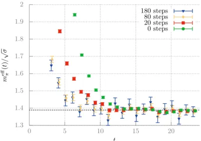
For negligible excited state contributions one would expect eq. (3.49) to hold exactly, i.e. m_eff should be a constant. A deviation from a constant will reveal the presence of excited state contamination. In fig. 3.2 we plot the effective mass for a pion, where the operators have been smeared both at source and sink, for an increasing number of steps.

1.3 1.4 1.5 1.6 1.7 1.8 1.9 2

0 5 10 15 20

meff π(t)/√ σ

t

180steps 80steps 20steps 0steps

Figure 3.2.: Effective mass for anSU(7)pion withm_π ≈ 620MeV. Different choices of smearing steps are shown.

While all the curves tend to the same plateau, the most smeared ones reach it earlier (i.e. for smaller values of t), though at the price of larger statistical errors. For this reason, both non-smearing and over-smearing are not advisable. To get rid of the higher states contribution, we look at the effective mass to establish the safe fitting region (see the next section) but we fit the correlator to eq. (3.49), instead of fitting the effective mass.

(27)

3.11. Variational method

The methods described so far allow to extract only the ground state from a given correlator, with a precision that depends on the overlap between the operator and the physical state. In order to extract the ground state and the first excited level we employ the variational analysis discussed in refs. [34–36]. For each channel, we computed the cross-correlation matrix,

Cij(t) =hOi(t)Oj(0)i (3.53) whereiandjcorrespond to the number of iterations (0,20,80or180steps in our case) of Wuppertal smearing, for the sources and the sinks.

Then we solved the generalized eigenvalue problem:

C(t)v^α=λ^α(t)C(t0)v^α (3.54) to extract the eigenvaluesλ^αwhich, as shown in ref. [35], behave as,

λ^α(t) =λ^α₀e^−tE^α 1 +O(e^−t∆E^α)

(3.55) fort N_tawith E_α = m_α for ~p = 0and ∆E_α being the mass gap to the next state (higherα-values indicating higher states). For the largest and second largest eigenvalues, λ⁰ and λ¹, we apply the same techniques explained in the previous section for C(t), i.e. we extract the massmperforming hyperbolic-cosine fits in[t_min, t_max]ranges (t_max≤aN_t/2) according to,

λ(t) =A

e^−mt+e^−m(aN^t^−t)

. (3.56)

All statistical uncertainties were estimated using a jackknife procedure. With four different operatorsOi, in many cases we were able to extract the first three states, however we regard the second excited states as unreliable at the present statistics. Using a subset of three operators out of the four mentioned above leads to compatible mass values within errors.

Varyingt0in the range[0,2a]gives compatible results, so we usedt0 =a. To select the best fit ranges, for each particle we first studied the effective mass defined in eq. (3.52), replacingC(t)withλ(t). We determinedtminas the Euclidean time separation at which m_eff reaches a plateau (within statistical uncertainties), so that the contribution from higher states is negligible, while t_max ≤ aN_t/2 is the value where m_eff becomes too noisy for stable fits. The signals become more precise at largerN, lowerκ-values (i.e.

larger quark masses) and are most precise for the pion and rho channels. Typically we fitλ(t) in the range[5a, aN_t/2]for the ground states and in the range[5a,10a]for the first excited states, adjusting these ranges (by one or two lattice spacings) on a case-by- case basis. Fitting to eq. (3.56) with this procedure leads to reducedχ²-values which are well below one.

(28)

The cost of inverting the propagator increases at lower quark masses, with the signal becoming noisier at the same time. For this reason, for the lowest two quark masses of eachSU(N) group, we focused only on the ground states and instead of using the variational method we computed the two point functions using80steps of smearing for the sources/sinks⁶. We then applied the same analysis forλ(t)directly to the correlator C(t).

3.12. String tension σ

Phenomenologically, we can model mesons by assuming that the valence quark and antiquark in a meson are tied together by a linearly rising potential. The simplest way to describe such a behaviour is to assume that the infrared regime of QCD is described by an “effective" string which joins together quark and antiquark.

In the real world the best set up to extract experimental information on the string tension σ is represented by the spectrum of the heavy quarkonia where the quark- antiquark spectrum can be studied with non-relativistic techniques thanks to the large masses of the quarks. Suitable potential models can be used to fit the spectrum and in this way a phenomenological estimate forσ≈1GeV/fm can be extracted.

R T

q q

Figure 3.3.: The Wilson loop

around a R×T

rectangle.

On the lattice the simplest way to mimic a static quark-antiquark pair is by studying the expectation value of a large rectangular Wilson loop of sizesR×T as shown in fig. 3.3. The physical in- terpretation of the expectation valuehW(R, T)iis that it represents the variation of the free energy due to the creation a the time t0 of a quark and an anti-quark which are separated by a distanceR from each other, evolve for a timeT, and finally annihilate at the instantt0+T.

According to this description we expect that for largeT:

hW(R, T)i ∼e^{−T V}^(R) (3.57) whereV(R) is the potential energy of the quark- antiquark pair. A way to estimate its value is:

V(R) =− lim

T→∞

∂

∂T loghW(R, T)i (3.58) In numerical simulations of non-Abelian Yang-Mills theory at zero temperature, Wilson loops of asymptotically large sizes are always found to obey an “area law”:

6Usually one has to smear more at smaller lattice spacing. In the section related to the continuum limit, we used 180 smearing steps and slightly largertminvalues for the very smallest lattice spacing.

(29)

hW(R, T)i=e^{−σ R T+...} (3.59) The area law for the Wilson loops is responsible for a linear rise of the potential:

V(R) 'σR, which implies linear confinement of static color sources, and the quantity σtakes the name “string tension”.

The string tensionσis an important quantity in lattice QCD, as it can be used to “set the scale” in pure gauge lattice simulations, i.e. to connect the values read on the lattice (pure numbers) to real-world quantities. In fact any quantity on the lattice is expressed in units of the lattice spacinga, which needs to be converted in physical units (fm). On the lattice we can measure:

a√

σ=F_σ(β) (3.60)

where F_σ(β) is a pure number depending on β. If we assume thead hoc valueσ = 1GeV/fm≈(444MeV)²and if we remember that into natural units~c'197MeV·fm is defined to be1, we can extract the value ofa:

a= Fσ(β)

√σ = Fσ(β)

444MeV = Fσ(β)

444 197fm (3.61)

In the literature the numerical quantityF_σ(β)is usually known with a very good precision, for most of the used gauge group in 3 and 4 dimensions. It is important to notice that the physical valueσ ≈ (444MeV)² is extrapolated from real-world phenomenology, so, strictly speaking, it should be used only forSU(3)QCD in 4d. It is a common practice however to use this number for different theories and dimensions. Alterna- tively, it is always possible to convert lattice results to physical units using ratios of dimensionful quantities, as we will do below.

(30)

Simulations and results 4

This chapter is focused on the results obtained at one single lattice spacing to illustrate the techniques and analysis used for each particle. Results at different lattice spacing, as well as continuum limit extrapolations, will be detailed in chapter 5.

4.1. Setting the scale

In this work, we study theories withSU(N)internal color symmetry withN = 2,3,4, 5,6,7and17color charges; in each case we choose the coupling

β = 2N

g² = 2N²

λ , (4.1)

such that the (square root of the) string tension in lattice units a√

σ ' 0.2093 is the same for eachN. This could be done with high accuracy forN = 2,3,4and6, using the string tension calculations of ref. [6, 7], and forN = 5and7, using those of ref. [8].

Using thead hocvalueσ = 1GeV/fm, our lattice spacing corresponds toa≈0.093fm or a⁻¹ ≈2.1GeV. We stress again that in the real world where experiments are performed, i.e. n_f > 0,N = 3 6= ∞, the string tension is not well defined. This means that any absolute scale setting in physical units will be arbitrary and is just meant as a rough guide.

For the theory with SU(17) gauge group, there are unfortunately no string tension calculations available, so we extracted aβ-value from a fit of the QCDΛ-parameter in

(31)

4. Simulations and results

0 0.05 0.1 0.15 0.2 0.25

1/N² 0.01

0.015 0.02

Λ/√σ

linear fit N≥6 linear fit N≥5 quadratic fit N≥6 quadratic fit N≥5 N=17

Figure 4.1.:Λ-parameter estimates of eq. (4.2), in units of the square root of the string tension. The errors shown are propagated from those ofa√

σ.

Fit 3 points 4 points linear 208.45 208.16 quadratic 209.04 208.77

Table 4.1.: Fit results forβatN = 17.

the lattice scheme:

Λ≈a⁻¹exp

− 1 2b0λ(a⁻¹)

·

b0λ(a⁻¹)⁻_2b^b¹2 0 ·

1 + 1

2b³₀ b²₁−b^L₂b0

λ(a⁻¹) +. . .

, (4.2) with [37, 38]

λ= 2N²

β , b₀ = 11

3 (4π)², b₁ = 34

3 (4π)⁴, b^L₂ = 1 (4π)⁶

−366.2 +1433.8

N² − 2143 N⁴

. (4.3) Λ/√

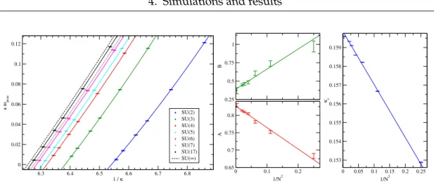
σ was calculated from the data presented in refs. [6–8] forSU(2 ≤ N ≤ 8)and is shown in figure 4.1. Using the data for N = 6, 7 and8 and a linear fit in1/N², we obtainedβ = 208.45forN = 17. Adding further values ofN ≥4or using a quadratic fit in1/N²changed this value by less than 0.3% (see table 4.1).

Table 4.2 summarizes the essential technical information of our computations. The N ≤7results presented in the fits and plots here are obtained from the24³×48lattices,