Public Transportation in Rural Areas: The Clustered Dial-a-Ride Problem

(1)

Master Thesis

Public Transportation in Rural Areas:

The Clustered Dial-a-Ride Problem

Fabian Feitsch

Date of Submission: October 5, 2018

Advisors: Prof. Dr. Sabine Storandt Prof. Dr. Alexander Wolff

Julius-Maximilians-Universität Würzburg Lehrstuhl für Informatik I

Algorithmen, Komplexität und wissensbasierte Systeme

(2)

Abstract

This thesis introduces theClustered Dial-a-Ride problem, which isN P-hard. In practice, the Clustered Dial-a-Ride problem occurs in the domain of public transportation in rural areas. Every village is represented by one cluster. A restriction of the structure of allowed solutions yields a fixed parameter algorithm whose parameter represents the size of the clusters. This makes the Clustered Dial-a-Ride problem solvable faster in practice than the original Dial-a-Ride problem. It turns out that the restriction on the set of solutions does in many realistic cases not play a role. In order to decide whether a specific instance allows the restriction, a classifier is presented. Experiments show that the classifier becomes more accurate the wider the villages lie apart. The classifier’s recall is above 80 percent for instances with six passengers and a mean distance of eight kilometers between the villages.

Zusammenfassung

Diese Arbeit führt dasClustered Dial-a-Ride Problem ein, welchesN P-schwer ist. In der Praxis taucht das Clustered Dial-a-Ride Problem bei der Umsetzung von öffentlichem Nahverkehr im ländlichen Raum auf, wobei Ortschaften durch Cluster abgebildet werden.

Durch eine Einschränkung der erlaubten Lösungen wird ein Festparameter-Algorithmus möglich, dessen Parameter die Größe der Cluster ist. Damit ist das Problem in der Praxis schneller lösbar als das traditionelle Dial-a-Ride Problem. Experimente zeigen, dass die Einschränkung der Lösungsmenge in vielen realistischen Fällen keine relevante Rolle spielt. Um zu entscheiden, ob eine gegebene Instanz eine solche Einschränkung erlaubt, wird ein Klassifikator präsentiert. Der Klassifikator wird akkurater, je weiter die Ortschaften auseinanderliegen und erreicht eine Trefferquote von über 80 Prozent für Instanzen mit sechs Passagieren und mittleren Abständen von acht Kilometern zwischen den Ortschaften.

Acknowledgement

Working on this thesis was real fun and I am grateful for the support I received by the members of the Chair, especially by Sabine Storandt. I thank also my partner Sonja Hohlfeld for the solace in times the programs made what I said they should do instead of doing what I meant them to do. Thanks also go to my father, Dieter Feitsch, who proofread the thesis and with whom I had the one or other fruitful discussion.

(3)

1 Introduction

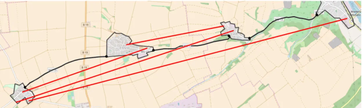
Fig. 1.1: A traditional bus line through villages. The red lines indicate walking distances of customers.

Bus stops are lousy. Often, they must be reached by foot. Sometimes, one feels insecure waiting at night for the bus. Always, standing at a bus stop is wasted time, which becomes even more inconvenient if the weather becomes unfriendly. In the city, these aspects are not as severe as in villages: The density of bus stops is higher, therefore walking distance is reduced. There are lights and other people around. And bus stops in the city are highly frequented, so the waiting time is not that long. Nowadays, villages are often connected to the cities with traditional bus lines using normal bus stops, even though the thoughts above indicate that standard bus lines are not well suited to be used in less densely populated areas.

This thesis suggests a different mode of public transportation in rural areas. As mentioned above, bus stops are often only located on the main street of the village and the walking distance to the bus stop can be very long. Figure 1.1 shows such a situation. The bus line goes from south to north and the colored dots indicate source and destination of the customers. The red lines show the distance they have to walk to and from the bus stops. However, it is not helpful to increase the density of stops inside the villages. The buses had to drive detours through the village to serve those stops even if no customer is waiting there. Due to the small number of customers this is supposed to happen often.

The complementary means of transport solves these problems: By using taxi cabs, the customers can be fetched at their doorstep and brought exactly to their destination. No time is wasted at the bus stop and there is no need to walk through raining weather. But taxi cabs are nor as cheap as public buses neither are they very environment-friendly because they carry only one passenger at once.

(5)

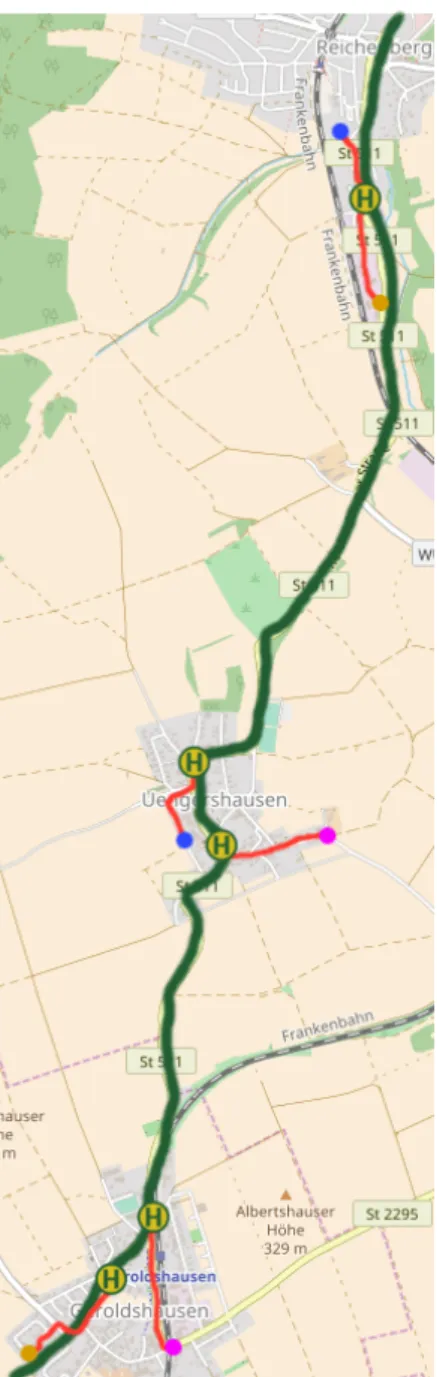
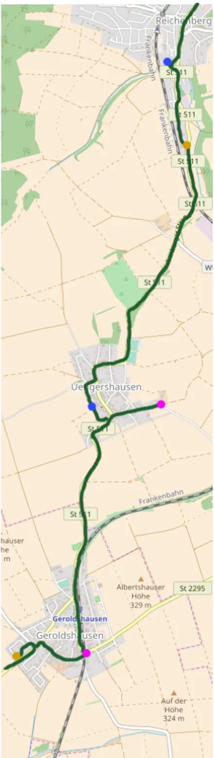
Fig. 1.2: The optimal route to serve the customers from the doorstep. It is only slightly longer than the traditional bus line.

It turns out that a combination of both means of transport is sensible: The customers are served not at static bus stops but rather at their precise venues, yet, unlike taxi cabs, other passengers may board or un- board during the journey. Naturally, the customers do not want to experience big detours to fetch or deliver foreign people, but they may accept little deviations of the shortest path. An instance is shown in Figure 1.2.

The customers are identical to Figure 1.1, but the vehicle serves the customers directly at their venues. The detours experienced by the the customers are small:

The yellow customer is on board while fetching the vio- let customer in the southern village. The extra journey for the blue dot in the northern village is still more neglectable.

The task of finding a route that minimizes the sum of all detours to serve a set of customers is called theDial- a-Rideproblem. Unfortunately, this problem is known to be computationally hard because it is a close relative to the well known Traveling Salesperson Problem.

This and other kinsmen are glanced onto in Section 2.

There exist slow exponential time algorithms to solve the Dial-a-Ride problem which are described in Chap- ter 3. However, there is one observation which makes the case at hand special: All customers are located inside villages. Intuitively, the cheapest tour is supposed to serve the villages along the main roads. This property would make the problem easier than the general variant. But the intuition is wrong. There are cases in which the optimal tour does not use the main road connecting the villages unidirectionally. Instead, it goes back and forth between the villages. In order to grasp and describe such instances the Clustered Dial-a-Ride problem is introduced in Chapter 4. In the same chapter, the central contribution of the thesis can be found:

A classifier which decides for a given set of customers and villages if the optimal tour is unidirectional. Chap- ter 5 explains how the algorithms presented in the two proceeding chapters were implemented technically and Chapter 6 examines realistic examples and evaluates the classifier. The last section of the thesis concludes the findings made in the preceding sections and gives proposals to future work.

(6)

2 Related Work

The introduction used the term Dial-a-Ride problem, which is the central algorithmic topic of this thesis. This chapter locates the Dial-a-Ride problem in its surrounding literature.

When talking about the Dial-a-Ride problem, one must take care because there are many different variants discussed in literature. The most basic of these variants resembles the Traveling Salesperson Problem (TSP) very strongly [31]. In a (euclidean) TSP instance, there are several points in the plane. The task is to find a roundtrip through all points that is as short as possible. This roundtrip must not contain any junctions or branches. The problem is very hard to solve and it remains hard even if only a simple path (not a roundtrip) is wanted. A small modification of the TSP is to organize the points in ordered pairs. For every pair, an order is defined in which both points of the pair must be visited. This variant of the TSP is the simplest representative of the Dial-a-Ride problem. It is also called TSP with Pickup and Delivery (TSPPD).

The goal remains to find the shortest path containing all points, but the visiting order must be maintained. This problem can be generalized to the TSP with Precedence Constraints, where the order of some points (not necessarily pairs) must be obeyed [2].

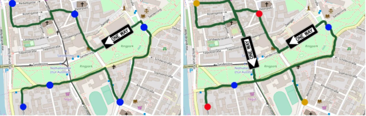
Figure 2.1 shows a normal TSP instance and a TSPPD instance. It is easy to see that the route solving the TSP instance does not solve the TSPPD instance. In 2008, Irina Dumitrescu et. al. tackled this variant of the Dial-a-Ride problem with an ILP based branch-and-cut algorithm [13]. Their algorithm is able to solve instances of up to 35 pairs in several minutes, more than doubling previous results [23]. But this TSPPD setting neither does punish detours of customers nor obeys the number of seats in the vehicle. These two additional constraints, however, occur relatively early in the history of the TSP. In 1959, the father of linear programing, Georg Dantzig, formulated the Vehicle Routing Problem (VRP) [8]. The task is to deliver a certain amount of goods from a fixed depot to customers. He introduced a capacity constraint for the vehicles and solves the problem with ILP, too. The paper also mentions that other constraints and target functions can be incorporated easily into the VRP. For example, one can add a last-in-first-out requirement on the tour. In this setting, every unloading must occur in reverse order of the loading. Jean-François Cordeau solves this kind of problem with a branch-and-bound algorithm [4]. On the other hand, it is also possible to ask for the first-in-first-out property where the first customer to be fetched must also be the first customer to be delivered. Ideas to solve this problem can be found in work by Carrabs et al. [3].

Most of the publications mentioned above focus on the transportation of goods. They mainly optimize and restrict the feasible routes in a way that allows efficient cargo delivery. If paying customers are to be transported, then other aspects become important and

(7)

Fig. 2.1: The left image shows a TSP instance and a route visiting all points. In the right image, the points are paired. For every pair, the left point has to be visited before the right point. The tour of the TSP can not be used to visit the points in the correct oder.

the problem is refered to as Dial-a-Ride problem. In 1980, Harilaos Psaraftis augmented the well known Held-Karp algorithm [18] for solving the TSP problem so that it is able to compute an optimal route for the Dial-a-Ride problem with sophisticated constraints and target functions [29]. Originally, his implementation obeys a capacity constraint and punishes detours as well as waiting times of the customers. It also incorporates an order in which the customers requested the service. This ensures that no customer waits forever if other customers at more convenient locations keep posting requests. How- ever, it is easy to change constraints and target function in Psaraftis’ algorithm without making it more complex. In Section 3.2, this algorithm is explained in detail. It is the fundamental algorithm of this thesis.

The aforementioned variants of the TSP problem, including the Dial-a-Ride problem, share the property that they are NP-hard. A reduction from TSP (which is known to be NP-hard [15]) to the TSPPD works as follows: Take a TSP instance and duplicate every vertex so that the original vertex and its copy reside in the same location. For every such pair any feasible route must visit the original vertex first, then its copy. Every tour in the TSPPD instance can be transformed into a TSP tour by deleting the copy vertices.

In the optimal TSPPD tour no detours are made because every pair of vertices is visited consecutively. Consequently, the reduction can also be used to show the NP-hardness of the Dial-a-Ride problem, which incorporates the minimization of detours in its objective function.

The Dial-a-Ride problem is part of the algorithmic scope of the ride sharing problem.

This problem is characterized by drivers owning vehicles and offering tours between two locations and customers without vehicles who search a suitable offer to travel to their destination. Examples for ride sharing platforms are BlaBlaCar [27] and Uber [22]. How- ever, their applications are different from the Dial-a-Ride or TSPPD problem described above. The main task of those platforms is to match requests to offers such that the detours of the offering drivers are not too big. A method to find a good matching is presented by Geisberger et. al. [16]. Their algorithm is meant to be applied by ride sharing platforms mainly addressing private drivers wanting to reduce the costs of single

(8)

journeys. On the other side, there are companies like Uber, as well as traditional taxi companies, which have to assign requests to their vast fleet of vehicles in real time. Often, these companies operate in metropolitan areas where it is desirable that the customer is fetched only minutes after posting the request. For these high-demand environments Alonso-Mora et. al. propose a heuristic matching method [1].

After the matching of offers and requests is done, the actual route is either computed with an exhaustive search (if the capacity of the vehicle is small), or heuristics are used [1]. Another way to find a route after the matching has been done is to agree on one single destination [26]. This use-case is motivated by touristic points of interests.

Several tourists traveling to a city together agree on one venue in the city where they all start their sightseeing tour individually.

As can been seen, the Dial-a-Ride problem is only a subproblem of the bigger setting of ride sharing. However,exact algorithms to find the optimal route once the requests have been matched to offers are rarely used. In the rural setting of this work, the matching of requests is done naturally because the village is served by one bus line and for every customer inside a village it is clear which line to use. If the bus line is replaced by a more dynamic vehicle, it is still clear which customer has to take which vehicle. This thesis does not cover changing bus lines during the journey. However, it can be useful to aggregate customers with many small vehicles to a assembly point where they transfer to a bigger vehicle. Drews and Luxen [12] examine ride sharing with hops. However, they pose two limitations on their approach: The hopping stations are pre-defined and the capacity of the vehicle being regarded is two. It is not clear whether their approach can be incorporated in the Dial-a-Ride instance considered in this thesis.

As mentioned in the introduction, the goal of this thesis is not only to solve the Dial- a-Ride problem, but to exploit the fact that all customers are located inside villages.

In other words, the instances to be solved are clustered. The author is not aware of any existing literature about the Clustered Dial-a-Ride problem. However, there is work on the clustered version of the traditional TSP problem (CTSP). In CTSP, the points are partitioned in predefined clusters and all points inside one cluster must be visited consecutively. Ding et. al. present a genetic algorithm that gives good heuristic results on CTSP instances [10]. Unfortunately, the optimal TSP tour through a CTSP instance often does not obey the clusters, so the lengths of the shortest routes of TSP and CTSP differ in general. Another approach is to find the clusters while computing a good TSP tour. Schneider et. al allow small deteriorations of the optimal route [30] while computing natural clusters. However, despite their similar nature to the Dial-a-Ride problem in rural areas, both approaches are not useful to find exact solutions.

The next section formulates the Dial-a-Ride variant used in this thesis in detail. Then, three different approaches to solve the Dial-a-Ride problem are presented. The clustered variant of the Dial-a-Ride problem is covered in Section 4.

(9)

3 The Dial-a-Ride Problem

As shown in the last chapter, the name Dial-a-Ride problem is not unique and there are many different ways to optimize a route. There are also various ways to limit the number of feasible routes, for example by defining ordering constraints or introducing vehicle capacities. This chapter describes the precise nature of the Dial-a-Ride problem concerned in this thesis. Then, the algorithm developed by Psaraftis [29] is explained in detail. This algorithm is already very powerful, but its recursive structure has some disadvantages, especially in storage management. A non-recursive variant is presented in this chapter, too, which admits a more economic usage of space. The last section of the chapter consists of a excursion to an ILP formulation of the Dial-a-Ride problem.

3.1 Problem Definition

The central part of all variants of the TSPPD, respectively. Dial-a-Ride problems are the customers. In literature, there are often called riders. Apart from the riders, a special person is introduced: the driver conducts the vehicle. A Dial-a-Ride instance is a triple I = (n, S,[di,j]). The variable n is the number of riders, S is the number of seats in the vehicle being used. Every person contributes two points to the instance, her pickup point and her dropoff point. The exact coordinates of these points are not relevant but rather the distances between all pairs of points (i, j) play an important role.

They are stored in the distance matrix [di,j]. Since there are n riders plus one driver, there are 2n+ 2 different points. Letm=n+ 1 be the number of persons in the instance.

Hence, the distance matrix has the size 2m×2m. Technically, the numbernis encoded in the size of the matrix [di,j] but stating n explicitly in I makes its relevance clearer.

Similar as in Psaraftis’ work, all points induced by I are ordered in a special way: The location with index 0 always refers to the starting point of the driver, and the location with indexmis his target point. The pickup point of the first rider has index 1 and the dropoff point of the first rider has index m+ 1. Generally, the pickup point of the ith rider is found at indexiand the corresponding dropoff point at indexm+i. Notice that the riders are counted starting from 1, since 0 is reserved for the driver. The following example makes this indexation clear.

Example. Let n = 5, i. e. there are five riders. Then there are 12 points in total and [d_i,j] has size 12×12. The entryd[4,7] refers to the distance between the pickup point of the forth rider and the dropoff point of the first rider (since 1 = 7−n+ 1 = 7−m). On the other hand, the entryd[4,9] is the distance between the pickup and dropoff location of the forth rider.

(10)

A location (ofI) is an element from the interval [0, . . . ,2m−1]. Atour orroute T is a permutation of all locations. Let pT(i) be an indicator variable which is 1 if the ith step of a tour is a pickup point; steps being counted starting from 1. Analogously,d_T(i) indicates whether theith step is a dropoff point. Both values can be computed easily:

p_T(j) =

(1 if T[j]< m

0 else d_T(j) =

(1 if T[j]≥m

0 else = 1−p_T(j)

Then k_T(i) = ^Pⁱ_j=1p_T(j)−d_T(j) counts the number of persons inside the vehicle after the ith step of a route T. The route T is feasible if three conditions are met.

First, it begins with location 0 and ends with location m. Second, for dropoff point d inT, the corresponding pickup point p=d−m must precededin T. Third, for every possible step 1 ≤ i ≤ 2m the inequality k_T(i) ≤ S must hold. These constraints result in the following properties which all feasible routes share (givenn >0): kT(1) = 1 since the driver is boarded first, k_T(2) = 2 because the second step must always be a pickup,k_T(2m−1) = 1 follows from the last rider to be dropped andk_T(2m) = 0 marks the end of the journey.

Example. Let T = [0,1,2,6,3,7,5,4] be a route. Since T consists of 8 steps, m = 4.

After picking the first rider (1), the second rider is picked (2). Then the second rider is dropped (2 + 4 = 6) and the third rider is picked (3). In the sixth step, the third rider is delivered (7). On all these journeys rider 1 was in the vehicle and is not dropped until the last-but-one step (5). Consequently, this route is only feasible ifS ≥3 since at most three persons are sitting in the vehicle at once. The routeT⁰= [0,7,2,6,3,1,5,4] is not feasible because rider 3 is dropped before she was picked.

Finding such a feasible route is easy. The permutationT = [0,1, m+1,2, m+2, . . . , m]

is always allowed. It means that every rider is fetched and delivered one after another, similar to taxi cabs. But this tour might not be satisfying. Naturally, one wants to minimize the costs of a tour T. There are three intuitive possibilities to define tour costs.

Distance being driven by the Driver Given a tourT, the distance driven by the driver is given by the following summation. Figure 3.1a shows an instance and a tour which optimizes this costs function.

c(T) =

2m

X

i=2

dT[i−1], T[i]

Finding the tour minimizing these costs may be useful if the entities being transported are goods. Humans, on the other side, do not want to travel along huge detours, especially to serve foreigners. Thus, this criterion is not used in this thesis.

(11)

0

1 2

6

3 7 5

4

(a) This route minimizes the distance driven by the driver. But the first rider is not happy

0

1 2

6

3 7 5

4

(b)This route minimizes the total distance that is driven. No rider is exposed to detours.

Fig. 3.1: A simple Dial-a-Ride instance with two different routes. The two locations belonging to the same rider are drawn with identical shapes. The numbers of the locations reflect the order of the locations inside the distance matrix [di,j]. In this example, all distances are euclidean.

Total Person distance driven Unlike the previous costs, the costs based on total distance contain the sum of all distances experienced by any person inside the vehicle. The resulting optimal tour can differ compared to the tour optimizing the previous costs, as depicted in Figure 3.1b. The costs function is realized by multiplying the distance with the number of persons inside the vehicle after every step:

c(T) =

2m

X

i=2

kT(i−1)·dT[i−1], T[i]

This costs function is sensible in the setting of this thesis because it does only punish detours, but not waiting times of the passengers. Waiting times need not to be taken into account because the aim of this thesis is to improve bus lines, which naturally have fixed departure times. Therefore, riders are willing to wait at home until they are fetched, even if the vehicle sometimes comes several minutes later than normal.

Total distance driven and waiting time The last costs function takes waiting times into account. The numbers of passengers waiting after step i of a route T is given by k⁰_T(i) =^P^2m_j=i+1p_T(j). Distance and waiting time are regarded to be equal. This is not quite accurate because the vehicle does not drive constant speed, but it simplifies the model without making totally insensible assumptions.

c(T) =

2m

X

i=2

kT(i−1) +k_T⁰ (i−1)·dT[i−1], T[i]

(12)

Psaraftis uses a deviation of this objective function in his original paper, which also incorporates a weighting between travel time and waiting time as well as a parameter describing customers’ preferences. As mentioned above, the second objective function suits better to the use case at hand. Thus, the total person distance driven objective is used in the thesis, except stated differently. All three objective functions evolve naturally from Psaraftis’ original objective function by setting selected parameters to 1 or 0, so no major modifications need to be made.

The first attempt to find an optimal route is to enumerate all feasible routes. As with its close relative TSP, this approach is not bearable for the Dial-a-Ride problem. Low values for the capacityS reduce the number of feasible routes, but it is easy to see that n! is a lower bound on the number of feasible routes ifS = 2: Serving the riders one after another yieldsn! possible routes. If S > m, then the exact number of feasible routes is given by the following theorem:

Theorem 3.1. Given n riders, there are Πⁿ_i=1(2i² −i) permutations in which every pickup occurs before the corresponding drop-off.

Proof. The theorem can be proven by induction. For n = 1 there is only one allowed permutation and 2·1²−1 = 1. The statement is proven for an arbitrary n under the assumption that it is correct forn−1. LetN be the number of permutations for n−1 riders. Since the statement is correct for n−1 the value for N is N = Πⁿ⁻¹_i=1(2i² −i).

Select one arbitrary permutationP of theseN permutations. Then there are^P^2(m−1)−1_i=1 i possibilities to incorporate an additional rider intoP. To see this, fix the pickup of the new rider to be after the first step of P, which is picking up the driver. Then there are 2(m−1)−1 ways to locate the dropoff in P because the last step cannot be a dropoff of a rider. In general, if the pickup is fixed to happen after the ith step in P, then there are 2(m −1)−i ways to arrange the dropoff. The sum accumulates the possibilities for every legal choice of i. Applying Gauss yields

2(m−1)−1

X

i=1

i= 2(m−1) 2(m−1)−1

2 = (2m−2)(2m−3)

2

= 4m²−10m+ 6

2 = 2m²−5m+ 3 = 2(m−1)²−(m−1).

There are N ways to select P, therefore, there are N · 2(m−1)² −(m−1) ways to serve an additional rider. Substituting m−1 with n yields the term N ·(2n²−n).

Since N = Πⁿ⁻¹_i=1(2i²−i), the number of feasible routes for nriders is Πⁿ_i=1(2i²−i).

It holds that Πⁿ_i=1(2i²−i)> n! andn!∈2^O(n^logⁿ⁾ for sufficiently largen. Thus, every exponential time algorithm has a better performance than this brute force approach.

Before such an exponential time algorithm is introduced, the definition of the Dial-a- Ride problem is extended. This extension makes it easier to understand the algorithms presented in the next section and is necessary in Section 4 where an algorithm is needed to solve Dial-a-Ride instancespartially.

(13)

1

0

2

3

4

5

6

7

8 9

Fig. 3.2: A feasible (possibly not the best) tour visiting only necessary locations of the partial Dial-a-Ride instanceI⁰ = (4, S,[finish,wait,travel,wait],[finish,finish,finish,wait]).

Therefore, the term partial Dial-a-Ride problem is defined. A partial Dial-a-Ride instance I⁰ = (n, S,[di,j],initial,final) is a quintuple. The first three properties are the same as in the normal Dial-a-Ride instance I. The new properties initial and final are both arrays of lengthn, indexed at 1. Every cell of these two arrays contains one element of {wait,travel,finish}. These elements encode states of the riders. A wait at location i means that the rideriis waiting at his pickup point. When the driveriis in the vehicle, then theith entry contains atravel. The element finishmeans that the rider is delivered.

Such arrays are referred to asstate vectorsorstate arrays in this thesis. Given a partial Dial-a-Ride instance I⁰, the goal is to find a cost optimal route through the locations such that when starting withinital, the states infinalevolve. The route still has to start at location 0 and end at location m.

Example. LetI⁰ = (4, S,[di,j],[finish,wait,travel,wait],[finish,finish,finish,wait] be a partial Dial-a-Ride instance. Theinital array states that the first rider is already delivered, the second and the forth rider are still waiting and the third rider is in the vehicle. The aim is to find a tourT such that after travelingT the first three riders are delivered and the forth rider is still waiting. All tours satisfying this property are permutations of the locations [0,2,5,7,8] because the other locations must not be touched. A sample tour is depicted in Figure 3.2.

Of course, theinitalandfinalstates must be compatible, otherwise there is no solution.

If wait > travel > finish, this condition can be expressed by initial[i] ≥ final[i] for every 1 ≤ i ≤ n. Given a normal instance I = (n, S,[di,j]), its corresponding partial version is I⁰ = (n, S,[d_i,j],[wait]ⁿ,[finish]ⁿ). Although the ordering of the locations and the state vectors were introduced by Psaraftis, his work did not mention partial Dial- a-Ride instances. Despite that, his algorithm can natively compute partial Dial-a-Ride instances without major modifications. Because his algorithm plays an important role in this thesis, the entire next section is dedicated to his algorithm. However, Psaraftis did restrict the set of feasible routes by obeying the order in which the riders posted their requests. For example, the fourth rider that posted a request must be picked up between steps 4−cand 4 +c wherecis a constant. This restriction does not take place in this thesis because it does not fit to the use case addressed in Chapter 4.

(14)

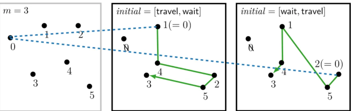
0

1 2

3

4 5

initial = [travel,wait]

0

1(= 0)

2 3

4

5

initial = [wait,travel]

0

1

2(= 0) 3

4

5 m= 3

Fig. 3.3: The left box shows a Dial-a-Ride instance I, the other two boxes show partial in- stanesI⁰ in which the location 0 was moved accordingly. The optimal route forI can be obtained by comparing the sum of costs of connecting location 0 to the subroutes and the costs of the subroutes themselves.

3.2 Psaraftis’ Algorithm

When thinking about the partial Dial-a-Ride problem, one can recognize the recursive nature of the problem. LetI = (n, S,[di,j]) be a Dial-a-Ride instance. Suppose that the firstisteps of the optimal tourT^∗are known and the remaining steps are still unknown.

The goal is to find an optimal tour through the remaining locations only. This task can be represented as a partial Dial-a-Ride instance whose initial state is defined by the already visited locations. This thought results in an approach to solve I: Guess the second step ofT^∗ (the first is always visiting location 0) and solve the remaining partial instance recursively. There are nguesses in total, of which the best one is chosen.

An example with two riders is shown in Figure 3.3. The leftmost box shows the original instance, the two other boxes show the optimal tour with the second step being guessed.

Since partial Dial-a-Ride instances have to start at location 0, too, the location 0 was artificially moved to location 1 and 2 in the recursion. Every recursive call reduces the complexity of the problem by one location. As soon as the there is only one location left, the sub-problem can be solved trivially.

This structure invites to use the dynamic programing technique, where a problem is reduced to several smaller problems of the same kind, which are computed and than incorporated into the main result [5]. Psaraftis’ algorithm essentially works as sketched above, however, it uses a more elegant way to reduce the problem instead of moving locations around.

The algorithm of Psaraftis is a recursive algorithm. It employs a global associative map V: [0, . . . ,2m−1]× {finish,travel,wait}ⁿ →R which assigns a rational number to a combination of a location index and a state array. The number V[l, s] represents the minimal costs for reaching thefinal state and then traveling to locationmwhen starting with the location land state s.

(15)

Algorithm 1:Psaraftis’ Algorithm to solve the Dial-a-Ride problem Input: A partial Dial-a-Ride instance I⁰

Output: The costs of the cheapest route to solveI⁰

1 (n, S,[di,j],initial,final) =I⁰ // Extract partial instance I⁰

2 V = new Map() with all entries being initially∞ // Initialize global map V

3 PsaraftisRecursive(I⁰, 0 , initial) // Call the recursive method

4 return V[0,initial]

Example. Iffinal= [finish]ⁿthenV[6,[travel] + [finish]ⁿ⁻¹] represents the optimal costs when starting at location 6, then delivering the first rider and than driving tom. Notice that m < 6 in this instance because all pickups have clearly been visited. The exact value ofV[6,[travel] + [wait]ⁿ⁻¹] is 2d[6,1 +m] +d[1 +m, m], because on the second last leg of the route, two persons are inside the vehicle and the last leg is only driven by the driver.

Psaraftis’ algorithm populates V with the correct values such that the properties above are fulfilled after the completion of the algorithm. At that moment, the costs of the optimal route for an instanceI = (n, S,[di,j]) is found in the cellV[0,[wait]ⁿ]. For partial instancesI⁰ = (n, S,[d_i,j],initial,final) this value is located in the cellV[0,initial]. The algorithm consists of two methods. The first method is a wrapper method that starts a recursion. The second method does the main work and is recursive. These two methods are shown in detail in Algorithm 1 and Algorithm 2. The two pseudocodes do not repeat the original algorithm but rather present a modified version which suits better to the Dial-a-Ride problem investigated in this thesis. The basic idea however was formulated by Psaraftis [29].

Algorithm 2 works as follows. The first if-statement checks that the current state does not violate the capacity constraint. The second if-statement abbreviates the calculation in case the value has already been computed. The third if-statement cancels the recursive algorithm in case the final state is reached. In this case, the cheapest value is only the distance of the current locationito the destination of the driverm, which is saved inV. Otherwise, the computation starts from scratch in the for-loop. The idea is to generate all states which may follow fromiandstate, compute their optimal values and select the successor which yields the minimal costs in combination with iand state. This is done by filtering all state entries which are not yet finished. For each of those entries a new location i⁰ a new state state⁰ are constructed. The new state advances the respective rider to the next stage. To this end, the ^↓-operator is utilized. It is a shorthand for a conditional statement and has the following semantic: wait^↓ =travelandtravel^↓=finish.

Then the recursive calculation is started. At the end of the loop, the best value is saved inV.

The algorithm always terminates because every recursive call represents a smaller instance, until the instances are so small that they are trivial to solve. The running time of the algorithm is O(n²3ⁿ⁻¹). There are 2n3ⁿ⁻¹+ 2 entries in V because there are 2n+2 locations. Except for locations 0 andm, there are 3ⁿ⁻¹allowed states for every

(16)

Algorithm 2:PsaraftisRecursive(I⁰,i,state)

Input: A partial Dial-a-Ride instance I⁰, a location indexiand a state arraystate Output: Costs of cheapest route starting atiwith statestate, ending atfinal ofI⁰

1 (n, S,[di,j],initial,final) =I⁰ // Extract the partial instance I⁰

2 k = Count occurrences of waits instate // Does not contain the driver.

3 if k+ 1> S then return

4 if V[i,state]<∞ then return // Value is already cached.

5 if final ==state then

6 V[i,state] =d[i, m]

7 return

8 v=∞

9 foreach index,entry∈state do

10 if entry==final[index]orentry ==finishthen

11 continue

// The “:” inside arrays is Phython’s slice notation.

12 state⁰ =state[:index] + [entry^↓] +state[index+1 :]

13 i⁰ =

(index ifentry ==wait

index+m ifentry ==travel // Computing new location.

14 PsaraftisRecursive(I⁰,i⁰,state⁰)

15 if (k+ 1)·d[i, i⁰] +V[i⁰,state⁰]< v then

16 v= (k+ 1)·d[i, i⁰] +V[i⁰,state⁰]

17 V[i,state] =v

location because the location fixes the state for exactly one rider. Computing the value of a locationi and a statestate needsO(n) steps. The claimed running time follows.

The alert reader may have noticed that the algorithm described as above does not return the optimal tour, but only the value of the optimal tour. This is typical for dynamic programs. To obtain the actual optimal tour, a second associative map P is introduced. This map stores parents of V’s key values. Every time a value v is stored in V, the location and state that caused v are saved in P. Thus at the end of the algorithm P contains pointers. Starting with P0,[wait]ⁿ, traversing the pointers and thereby collecting the locations until the location m is reached yields the actual tour.

The algorithm of Psaraftis’ is the fundamental algorithm of this thesis. However, the experiments that were conducted are based on another variant of Psaraftis’ algorithm than described above. This variant and the reasons for using it instead of the original algorithm are discussed in the next section.

(17)

0

1

2

4

2

1

5

2 4 5 4 5 1

5 5 4 5 4 4

3 3 3 3 3 3 1

1

2 2

1

3 3

1

2

2 2 2 2

2

1

1 1 1 1

1

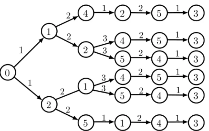
Fig. 3.4: A complete decision tree for two riders. The numbers on the edges indicate the number of persons in the vehicle at the time the edge is taken. If S = 2, then the four inner branches would be pruned and there were only two feasible routes.

3.3 Incremental Variant of Psaraftis’ Algorithm

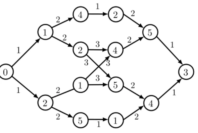
A natural way to approach the Dial-a-Ride problem is to illustrate the feasible routes as a decision tree. An example of such a tree for two riders is shown in Figure 3.4. The capacity S of this instance is ∞. In the first step, the driver can choose which rider to fetch first. Then he can either pick an additional rider or drop the recently boarded rider first. Every path in the tree represents a feasible tour. Remember that the locations are referenced by their indices. Thus, the leaves of such a decision tree must always contain the driver’s dropoff, which is m. In the example figure m = 3 because there are two riders. An algorithm that builds and evaluates such a tree would essentially be a brute force algorithm that enumerates all feasible routes. The number of leaves is predicted by Theorem 3.1. However, the tree can be compressed since many parts of the tree are redundant. Consider two vertices with the same depth that share the same set of predecssors, including themselves. For example, in Figure 3.4 both vertices of location 4 in the penultimate step have the same set of predecessors, but in different order. Everything that happens after these two vertices (i.e. to the right of them) is identical. Therefore, such vertices are merged. The compressed graph of Figure 3.4 is shown in Figure 3.5. Using the compressed directed acyclic graph, Psaraftis’ algorithm can be illustrated. It proceeds in a depth-first-search manor through the graph and computes the values from right to left. Every vertex in the graph is a recursive call. The parameteri can be found inside the vertex itself and the parameter state can easily be deduced from the predecessors of the vertex. Every edge is traversed exactly one time because cached values are reused.

Another possibility is to compute the values from left to right in a breadth-first-search manor. Starting with the leftmost vertex having value 0, the values of the successors are computed level-wise until the rightmost vertex is reached. The pseudocode is shown in Algorithm 3. A huge share of the algorithm is very similar to the original variant.

The main difference is the utilization of a queue to organize the commutated values instead of using recursion, which results in a different interpretation of the mapV. The

(18)

0

1

2

4

2

1

5

2

4

5

1

5

4

3 1

1

2 2

2

1

3

3 3

3

1

2

1

Fig. 3.5: The compressed variant of Figure 3.4. Again, the current vehicle load is shown on the edges. IfS= 2, the four paths through the center would not exist.

cellV[l,state] contains the costs that are at most necessary to reach locationland state vectorstate. The numbers inV decrease while the algorithm is running and are optimal by the end of the algorithm. It starts by setting V[0,initial] to 0 and storing it in a queue. The main for-loop extracts the states from the queue in first-in-first-out order.

For every extracted key all possible succeeding states are generated in the same way as the recursive variant does. However, infeasible states are discarded at once and only feasible states enter the queue. The if-condition in line 19 ensures that no location/state- pair can enter the queue twice. All entries that are removed fromQhave their optimal value already set. The overall optimal value is found in V[m,final]. Notice that the queue never contains more vertices than the number of maximal vertices in one vertical layer of Figure 3.4.

The reason why this algorithm is preferred over the algorithm from literature is that the author finds it more intuitive and better debugable than the original algorithm. Also, the incremental algorithm seemed to be faster in reality, even if the asymptotic running times are, of course, identical. This observation is not based on thorough benchmarking but rather on some quick checks. Another advantage of the incremental algorithm is that it offers a possibility to save space. While in the original recursive algorithm of Psaraftis every state must be kept because it may be needed later on, the incremental version need only keep two layers in the memory at once. If not only the value of the optimal solution has to be found, than the parents must be saved too, in the same way as they must be stored in the recursive variant. However, some of the states eventually can not be reached any more. These states can also be deleted. Thus, when the algorithm is implemented in a language that supports effective garbage collection, then the advantage of needing less memory than the recursive variant remains.

Despite these fundamental changes to the original algorithm, the idea stays the same.

Therefore, the term Psaraftis’ Algorithm refers to either of both variants in the remainder of the thesis. If the exact version is important, it will be stated at that point. Before turning to the Dial-a-Ride problem in rural areas, a quick excursion is done. The next section presents an ILP model for the Dial-a-Ride problem.

(19)

Algorithm 3:A variant of Psaraftis’ algorithm. It proceeds in breadth-first-manor.

Input: A partial Dial-a-Ride instance I⁰

Output: The value of the best tour to deliver all riders.

1 (n, S,[d_i,j],initial,final) =I⁰

2 Q= new Queue()

3 V = new Map() with all entries being initially∞

4 V[0,initial] = 0

5 Q.enqueue[(0,initial)]

6 while Q6=∅ do

7 i,state =Q.dequeue()

8 if state==final then

9 V[m,final] = min{V[m,final], V[i,state] +d[i, m]}

10 continue

11 foreach index,entry ∈state do

12 if entry==final[index]or entry==finishthen

13 continue

14 state⁰ =state[:index] + [entry^↓] +state[index+1 :]

15 k = Count occurrences of waits instate⁰

16 if k+ 1> S then

17 continue

18 i⁰ =

(index ifentry ==wait index+m ifentry ==travel

19 if V[i⁰,state] ==∞ then

20 Q.enqueue[i⁰,state⁰]

21 V[i⁰,state]⁰ = minV[i⁰,state⁰],(k+ 1)·d[i, i⁰] +V[i,state]

22 return V[m,final]

(20)

3.4 Excursion: An ILP for Dial-a-Ride Instances

Linear Programs are a popular technique to tackle optimization problems. If one is able the formulate the problem using linear inequalities and a linear objective function, an algorithm to solve the problem comes for free. The first algorithm to solve linear programs is Dantzig’s Simplex algorithm [7] which runs in polynomial time in most cases. Every Dial-a-Ride instanceI can be described as a linear program and the variable values computed by the solving algorithm can be translated into the optimal tour. Unfortunately, the Simplex algorithm assigns fractional values to variables so that their interpretation becomes ambiguous. The solution is to force all variables to be integer values. However, if a NP-hard problem is modeled as such an integer linear program (ILP), then solving the ILP becomes NP-hard, too. Thus there is little hope to solve the Dial-a-Ride problem in polynomial time using ILP (assuming P 6=N P). Even so, the Dial-a-Ride problem may be one of the problems for which solving the corresponding ILP is faster or easier than developing and running a combinatorial algorithm.

To check this conjecture and to verify the results of the other algorithms, a program was written to translate Dial-a-Ride instancesI into integer linear models. The program is written in the Optimization Programming Language [21], a language that creates models for the IBM ILOG CPLEX Optimization Studio [20]. However, it turned out that CPLEX needs much more time for solving an instance than the other two algorithms:

While Psaraftis’ algorithm needs only a couple of seconds to solve instances of sizen= 8, CPLEX did not finish after fifteen minutes. Both tests were run on usual desktop computers. Thus, the ILP implementation can be regarded as pilot study with little relevance for the remainder of the thesis. The author is aware that sophisticated methods to improve CPLEX’s (and similar algorithms’) performance exist, but this is not the main topic of the thesis. Ideas of utilizations of these advanced techniques for the Dial-a-Ride problem can be found in the work by Dumitrescu et. al. [13] and Cordeau [4].

The remainder of the section presents the integer linear model describing a Dial-a- Ride problem. It is important to note that in this linear model the driver is considered to be a rider which means that the rider r = 0 is the driver. Given a Dial-a-Ride instance I = (n, S,[di,j]), a linear model can be constructed as follows. Introduce a set of variables x^pick_i,r and a set of variablesx^drop_i,r for 1≤i≤2m and 0 ≤r < m and allow only values 0 or 1 for every variable. These variables are used to model the optimal tour. If the solver assigns x^pick_i,r = 0, then rider r is picked sometime after the ith step in the tour. If, on the other hand,x^pick_i,r = 1, then the rider is picked at or before step i.

Analogously,x^drop_i,r is interpreted. The consequence is that the position of rider r can be determined for every fixed step i. If x^pick_i,r = 0 and x^drop_i,r = 0 then the rider was not yet fetched at step i of the tour, ifx^pick_i,r = 1 and x^drop_i,r = 0, then the rider is in the vehicle at stepiand when both variables are 1, then the rider is already delivered. It is obvious that this distinction lacks one case: Logically, the case x^pick_i,r = 0 andx^drop_i,r = 1 cannot be interpreted because it contradicts the definition of the variables. This asks for a set of constraints that guarantee a feasible route. The following inequalities accomplish this goal. Be reminded that persons are 0-indexed and steps are 1-indexed.

(21)

x^pick_i,r ∈ {0,1} and x^drop_i,r ∈ {0,1} for alli∈[1,2m], r∈[0, m−1] (3.1) x^pick_i,r ≤x^pick_i+1,r and x^drop_i,r ≤x^drop_i+1,r for all i∈[1,2m−1], r∈[0, m−1] (3.2) x^drop_i,r ≤x^pick_i,r for alli∈[1,2m], r∈[0, m−1] (3.3)

m−1

X

r=0

x^pick_i,r +

m−1

X

r=0

x^drop_i,r =i for all i∈[1,2m] (3.4)

m−1

X

r=0

x^pick_i,r −

m−1

X

r=0

x^drop_i,r ≤S for all i∈[1,2m] (3.5)

x^pick_1,0 = 1 and x^drop_2m−1,0 = 0 (3.6)

The first line advises the solver of the linear program that all variables must be either 0 or 1. The second line ensures that once a variable for riderrat a fixed stepiis 1, then it stays 1 for the rest of the tour. In other words, the variables are monotonous with regard to the stepifor fixedr. Equation 3.3 forbids that a rider is dropped without being picked before. Technically, this would be the case ifx^pick_i,r = 0 andx^drop_i,r = 1. Therefore, it is required that the pick variable is always at least as big as the corresponding drop variable. In Equation 3.4 every step is forced to carry out exactly one action. This can be imagined as follows. Every time a person is picked or dropped in a feasible tour, exactly one variable becomes 1. For a certain step i, there must have been i actions carried out so far. Adding up all variables for this step has to be equal to i, otherwise too few or too many actions happened so far, which is not allowed. It must also be guaranteed that the capacity of the vehicle is never violated during the tour. Again, this task can be regarded step-wise. For a fixed step, the difference of pick-variabes and drop-variables denote the number of persons in the vehicle at step i, which must not be greater than S. Equation 3.5 realizes this requirement. The last two inequalities (Equation 3.6) distinguish the driver from the riders by forcing the driver to be the first person to be fetched and the last person to be delivered. To illustrate the interaction of these equations, an example with two riders and one driver is given in Figure 3.6. It can be seen that the assignment of the variables fulfill the equations and induce a feasible route. The complexity of the model so far isO(m²) variables andO(m²) constraints.

As mentioned earlier, it is easy to find a feasible route without an objective function.

Indeed, CPLEX produces feasible routes very fast if the objective function is not stated.

Unfortunately, the variables introduced above are not sufficient to state the desired objective function. Therefore, more variables are defined that are only needed to formulate the objective function. The long term aim is to define a variable x_(u,v),r being 1 iff person r was in the vehicle at the time the vehicle drove from location u to location v.

Using this variable, the objective function can be stated with Equation 3.7.

(22)

Person Variable i= 1 i= 2 i= 3 i= 4 i= 5 i= 6

Driver x^pick_i,0 1 1 1 1 1 1

x^drop_i,0 0 0 0 0 0 1

Rider 1 x^pick_i,1 0 1 1 1 1 1

x^drop_i,1 0 0 0 1 1 1

Rider 2 x^pick_i,2 0 0 1 1 1 1

x^drop_i,2 0 0 0 0 1 1

Location of Vehicle 0 1 2 4 5 3

Equation 3.4 1 2 3 4 5 6

Equation 3.5 1 2 3 2 1 0

Fig. 3.6: A feasible assignment of the x^pick_i,r and x^drop_i,r variables. The route induced by this assignment is: pick 0, pick 1, pick 2, drop 1, drop 2, drop 0. The last two lines illustrate the referenced constraints.

min ^X

(u,v)∈[0,2m−1]² m−1

X

r=0

x_(u,v),r·d[u, v] (3.7)

The matrix [d_i,j] is that of the instanceI. When a connection (u, v) is never used in a tour, the variablex_(u,v),r is 0 for every rider and the edge is not included in the objective value. The tuple (u, v) will be abbreviated as edge e in the remainder of the section.

This remainder explains howx_(u,v),r is realized.

Let e ∈ [0,2m−1]² be an edge between two locations. Then the value 1 should be assigned to the binary variable xi,e if the edge e is used directly after the ith step. In Figure 3.6 the edge (2,4) is taken between steps 3 and 4, so x_3,(2,4) = 1. Location 2 is the pickup location for the second rider and 4 is the dropoff location of the first rider.

In order to assign the correct value toxi,e it is important to distinguish four edge types:

An edge is either a connection between two pickup locations or two dropoff locations or a combination of them. This thesis explains how the value x_i,e is obtained for edges connecting two pickup locations, the other types work with the same argumentation.

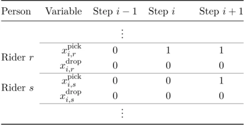
Let e = (u, v) be an edge with u and v both being pickup locations of riders r and s.

With other words, u < m and v < m, u = r and v = s. There is only one possible constellation which allows the vehicle to use edge e at step i. Figure 3.7 shows that situation. The values for the pick-variables must look like those depicted in the table.

The trick to formulate a constraint for x_i,e is to add up all variables that ought to 1 and to subtract all variables that must not be 1. If this calculation yields the value 3, thenxi,e must be 1. The values for the drop-variables can be ignored because they are forced to be 0 by the Constraints 3.2 and 3.3. Constraint 3.8 attempts to realizex_i,e.

(23)

Person Variable Step i−1 Step i Stepi+ 1 ...

Rider r x^pick_i,r 0 1 1

x^drop_i,r 0 0 0

Rider s x^pick_i,s 0 0 1

x^drop_i,s 0 0 0

...

Fig. 3.7: In this situation, the vehicle uses the edge (u, v) at stepi. There is no other way to assign the variables and keep the edge used in stepi.

x_i,e≥ −x^pick_i−1,r−x^pick_i−1,s−x^pick_i,s +x^pick_i,r +x^pick_i+1,r+x^pick_i+1,s−2 (3.8) for alli∈[2,2m−1], e∈[0,2m−1]²

The constraints for the other three types of edges have the same structure, the only difference is thatx^pickmust be replaced by x^drop accordingly. The variables of the form x1,e must be handled specially to avoid index out of bounds errors. It is granted that the first edge to be used connects location 0 and another pickup location (otherwise the instance could be solved trivially). Thus the variables x_1,(0,u) for arbitrary pickup locations u must be at least as great asx^pick_2,u . There must be oneu for which x^pick_2,u = 1 and the corresponding edge variable is forced to the correct value with Constraint 3.9.

x_1,(0,u)≥x^pick_2,u for all u∈[1, m−1] (3.9) These edge constraints introduce O(m³) new variables and O(m³) new constraints.

The alert reader may have noticed that there is a problem with the constraints stated above: The solver will set x_i,(r,r+m) = 1, independently from the assignment of the domain variablesx^pick_i,r and x^drop_i,r . The reason for this is that then all riders are delivered without any detours which clearly minimizes the objective function. The core problem is that in this case more edges are used than allowed. For m persons there can only be 2m−1 used edges in any feasible tour. The following constraint asserts this property and prevents the solver from using too many edges:

2m−1 = ^X

e∈[0,2m−1]² 2m−1

X

i=1

xi,e (3.10)

Notice that the edge variables also intentionally contain trivial edgese= (p, p). These variables are never assigned 1 and thus are not causing any harm. Moreover, it simplifies the notation.

(24)

Lett^pick_r ,t^drop_r be variables describing the step in which riderrwas picked or dropped.

The variablete represents the stepafter which ewas used, respectively. Be aware that these three kinds of variables are natural, not binary. The values of all three variable types are defined straight forwardly in the following three constraints. Since the steps are counted starting with 1, the variablest^pick_r and t^drop_r are incremented by 1.

t^pick_r = 2m−

2m

X

i=1

x^pick_i,r + 1 for all r∈[0, m−1] (3.11)

t^drop_r = 2m−

2m

X

i=1

x^drop_i,r + 1 for all r∈[0, m−1] (3.12)

te=

2m−1

X

i=1

xi,e·i for all e∈[0,2m−1]² (3.13) These three kinds of variables are the only variables that are not binary. This is unfortunate because these variables increase the space of possible solutions enormously.

It is possible to replace these real number variables with binary variables, but this meansO(m⁴) new variables instead of O(m) new variables and a lot more constraints.

Tests showed that the running times of the binary-only linear programs were not better than the running time of the model presented here. The author refrains from explaining the binary variant in this thesis.

Naturally, x_e,r = 1 iff rider r was picked before the edge e was used and dropped after it was used, i.e x_e,r = 1 ⇔t^pick_r ≤t_e < t^drop_r . In order to express this logical rule with linear inequalities two more auxiliary variables are needed. These variables reflect whether the two relation-signs in the latter term are fulfilled or not. Let x^pick_e,r be 1 iff personr was picked any time before the vehicle used edgee. Analogously, x^drop_e,r should be 1 iff personr was dropped any time after the vehicle used edgee. The correct values for these types of variables are implemented by the those constraints:

x^pick_e,r > t_e−t^pick_r

2m−1 for all e∈[0,2m−1]², r∈[0, m−1] (3.14) x^drop_e,r ≥ t^drop_r −t_e

2m−1 for all e∈[0,2m−1]², r∈[0, m−1] (3.15) Even though these terms include division it is a legal linear expression because 2m−1 is a constant in the realm of the model. Per definition, the result of Equation 3.14 lies in the interval ]−1,1[. The variable t^pick_r is at most 2m−2 because the last two actions must be dropoffs, and t_e is at least 0. Thus, the minimal value of the division is −(2m−2)/(2m−1)>−1. The maximal value is (2m−1−1)/(2m−1)<1. The result is negative if e was used before r was picked ore was not used at all, otherwise