Wireless Network Information Flow: A Deterministic Approach

(1)

Wireless Network Information Flow:

A Deterministic Approach

A. Salman Avestimehr, Member, IEEE,Suhas N. Diggavi, Member, IEEE, and David N. C. Tse, Fellow, IEEE

Abstract—In a wireless network with a single source and a single destination and an arbitrary number of relay nodes, what is the maximum rate of information flow achievable? We make progress on this long standing problem through a two-step approach. First we propose a deterministic channel model which captures the key wireless properties of signal strength, broadcast and superposition. We obtain an exact characterization of the capacity of a network with nodes connected by such deterministic channels. This result is a natural generalization of the celebrated max-flow min-cut theorem for wired networks. Second, we use the insights obtained from the deterministic analysis to design a newquantize-map-and-forwardscheme for Gaussian networks. In this scheme, each relay quantizes the received signal at the noise level and maps it to a random Gaussian codeword for forwarding, and the final destination decodes the source’s message based on the received signal. We show that, in contrast to existing schemes, this scheme can achieve the cut-set upper bound to within a gap which is independent of the channel parameters. In the case of the relay channel with a single relay as well as the two-relay Gaussian diamond network, the gap is 1 bit/s/Hz. Moreover, the scheme is universal in the sense that the relays need no knowledge of the values of the channel parameters to (approximately) achieve the rate supportable by the network. We also present extensions of the results to multicast networks, half-duplex networks and ergodic networks.

Index Terms—Information flow, network capacity, network information theory, relay networks, wireless networks.

I. INTRODUCTION

Two main distinguishing features of wireless communication are:

• broadcast: wireless users communicate over the air and signals from any one transmitter are heard by multiple nodes with possibly different signal strengths.

• superposition: a wireless node receives signals from multiple simultaneously transmitting nodes, with the received signals all superimposed on top of each other.

Because of these effects, links in a wireless network are never isolated but instead interact in seemingly complex ways.

A. S. Avestimehr is with the School of Electrical and Computer Engineer- ing, Cornell University, Ithaca, USA. Email:avestimehr@ece.cornell.edu.

S. N. Diggavi is with the Department of Electrical Engineering, UCLA, Los Angeles, USA. Email:suhas@ee.ucla.edu.

D. N. C. Tse is with the Department of Electrical Engineering and Computer Sciences, UC Berkeley, Berkeley, USA. Email:dtse@eecs.berkeley.edu.

The research of D. Tse and A. Avestimehr were supported in part by the National Science Foundation under grants 0326503, 0722032 and 0830796, and by a gift from Qualcomm Inc. The research of S. Diggavi was supported in part by the Swiss National Science Foundation NCCR-MICS center.

Manuscript received July 28, 2009; revised June 1, 2010 and August 5, 2010. Date of current version September 16, 2010.

Communicated by M. Franceschetti, Associate Editor for Communication Networks.

On the one hand, this facilitates the spread of information among users in a network; on the other hand it can be harmful by creating signal interference among users. This is in direct contrast to wired networks, where transmitter-receiver pairs can be thought of as isolated point-to-point links. Starting from the max-flow-min-cut theorem of Ford-Fulkerson [1], there has been significant progress in understanding network flow over wired networks. Much less, however, is known for wireless networks.

The linear additive Gaussian channel model is a commonly used model to capture signal interactions in wireless channels.

Over the past couple of decades, capacity study of Gaussian networks has been an active area of research. However, due to the complexity of the Gaussian model, except for the simplest networks such as the one-to-many Gaussian broadcast channel and the many-to-one Gaussian multiple access channel, the capacity of most Gaussian networks is still unknown. For example, even the capacity of a Gaussian single-relay network, in which a point to point communication is assisted by one relay, has been open for more than 30 years. In order to make progress on this problem, we take a two-step approach. We first focus on the signal interaction in wireless networks rather than on the noise. We present a new deterministic channel model which is analytically simpler than the Gaussian model but yet still captures three key features of wireless communication:

channel strength, broadcast. and superposition. A motivation to study such a model is that in contrast to point-to-point channels where noise is the only source of uncertainty, networks often operate in the interference-limited regime where the noise power is small compared to signal powers. Therefore, for a first level of understanding, our focus is on such signal interactions rather than the background noise. Like the Gaussian model, our deterministic model is linear, but unlike the Gaussian model, operations are on a finite-field. The simplicity of scalar finite-field channel models has also been noted in [2].

We provide a complete characterization of the capacity of a network of nodes connected by such deterministic channels.

The first result is a natural generalization of the max-flow min-cut theorem for wired networks.

The second step is to utilize the insights from the deterministic analysis to find “approximately optimal” communication schemes for Gaussian relay networks. The analysis for deterministic networks not only gives us insights for potentially successful coding schemes for the Gaussian case, but also gives tools for the proof techniques used. We show that in Gaussian networks, an approximate max-flow min-cut result can be shown, where the approximation is within an additive constant which is universal over the values of the channel

arXiv:0906.5394v7 [cs.IT] 25 Feb 2011

(2)

parameters (but could depend on the number of nodes in the network). For example, the additive gap for both the single-relay network and for the two-relay diamond network is 1 bit/s/Hz. This is the first result we are aware of that provides such performance guarantees on relaying schemes.

To highlight the strength of this result, we demonstrate that none of the existing strategies in the literature, like amplify- and-forward, decode-and-forward and Gaussian compress-and- forward, yield such a universal approximation for arbitrary networks. Instead, a scheme, which we term quantize-map- and-forward, provides such a universal approximation.

In this paper we focus on unicast and multicast communication scenarios. In the unicast scenario, one source wants to communicate to a single destination. In the multicast scenario source wants to transmit thesamemessage to multiple destinations. Since in these scenarios, all destination nodes are interested in the same message, there is effectively only one information stream in the network. Due to the broadcast nature of the wireless medium, multiple copies of a transmitted signal are received at different relays and superimposed with other received signals. However, since they are all a function of the same message, they are not considered as interference.

In fact, the quantize-map-and-forward strategy exploits this broadcast nature by forwarding all the available information received at the various relays to the final destination. This is in contrast to more classical approaches of dealing with simultaneous transmissions by either avoiding them through transmit scheduling or treating signals from all nodes other than the intended transmitter as interference adding to the noise floor. These approaches attempt to convert the wireless network into a wired network but are strictly sub-optimal.

A. Related Work

In the literature, there has been extensive research over the last three decades to characterize the capacity of relay networks. The single-relay channel was first introduced in 1971 by van der Meulen [3] and the most general strategies for this network were developed by Cover and El Gamal [4].

There has also been a significant effort to generalize these ideas to arbitrary multi-relay networks with simple channel models. An early attempt was done in the Ph.D. thesis of Aref [5] where a max-flow min-cut result was established to characterize the unicast capacity of a deterministic broadcast relay networkwithout superposition. This was an early precur- sor to network coding which established the multicast capacity of wired networks, a deterministic capacitated graph without broadcast or superposition [6], [7], [8]. These two ideas were combined in [9], which established a max-flow min- cut characterization for multicast flows for “Aref networks”.

However, such complete characterizations are not known for arbitrary (even deterministic) networks with both broadcast and superposition. One notable exception is the work [10]

which takes a scalar deterministic linear finite-field model and uses probabilistic erasures to model channel failures. For this model using results of erasure broadcast networks [11], they established an asymptotic result on the unicast capacity as the field size grows. However, in all these works there is

no connection between the proposed channel model and the physical wireless channel.

There has also been a rich body of literature in directly tackling the noisy relay network capacity problem. In [12] the

“diamond” network of parallel relay channels with no direct link between the source and the destination was examined. Xie and Kumar generalized the decode-forward encoding scheme for a network of multiple relays [13]. Kramer et al. [14] also generalized the compress-forward strategy to networks with a single layer of relay nodes. Though there have been many interesting and important ideas developed in these papers, the capacity characterization of Gaussian relay networks is still unresolved. In fact even a performance guarantee, such as establishing how far these schemes are from an upper bound is unknown. In fact, as we will see in Section III, these strategies do not yield an approximation guarantee for general networks.

There are subtle but critical differences between the quantize-map-forward strategy, proposed in this paper, with the natural extension of compress-forward to networks for the following reasons. The compress-forward scheme proposed in [4], quantized the received signal and then mapped the digital bin index onto the transmit sequence. This means that we need to make choices on the binning rates at each relay node.

However, the quantize-map-forward scheme proposed in this paper directly maps the the quantized sequence to the transmit sequence, and therefore does not make such choices on the binning rates. In fact this gives the scheme a “universality”

property, which allows the same relay operation to work for multiple destinations (multicast) and network situations (compound networks); a property that could fail to hold if specific choices of binning rates were made. Moreover, our scheme unlike the classical compress-forward scheme, does not require the quantized values at the relays to be reconstructed at the destination, while it is attempting to decode the transmitted message. These are the essential differences between our scheme and the traditional compress-forward, or the natural network generalization of it.

Our results are connected to the concept of network coding in several ways. The most direct connection is that our results on the multicast capacity of deterministic networks are direct generalizations of network coding results [6], [7], [8], [15], [16] as well as Aref networks [5], [9]. The coding techniques for the deterministic case are inspired by and generalize the random network coding technique of [6] and the linear coding technique of [7], [8], [17]. The quantize-map-and-forward technique proposed in this paper for the Gaussian wireless networks uses the insights from the deterministic framework and is philosophically the network coding technique generalized to noisy wireless networks.

B. Outline of the paper

We first develop an analytically simple linear finite-field model and motivate it by connecting it to the Gaussian model in the context of several simple multiuser networks. We also discuss its limitations. This is done in Section II. This model also suggests achievable strategies to explore in Gaussian relay networks, as done in Section III, where we illustrate the

(3)

deterministic approach on several progressively more complex example networks. The deterministic model also makes clear that several well-known strategies can be in fact arbitrarily far away from optimality in these example networks.

Section IV summarizes the main results of the paper. Sec- tion V focuses on the capacity analysis of networks with nodes connected by deterministic channels. We examine arbitrary deterministic channel model (not necessarily linear nor finite- field) and establish an achievable rate for an arbitrary network.

For the special case of linear finite-field deterministic models, this achievable rate matches the cut-set bound, therefore exact characterization is possible. The achievable strategy involves each node randomly mapping the received signal to a transmitted signal, and the final destination solving for the information bits from all the received equations.

The examination of the deterministic relay network moti- vates the introduction of a simple quantize-map-and-forward strategy for general Gaussian relay networks. In this scheme each relay first quantizes the received signal at the noise level, then randomly maps it to a Gaussian codeword and transmits it¹. In Section VI we use the insights of the deterministic result to demonstrate that we can achieve a rate that is guaranteed to be within a constant gap from the cut-set upper bound on capacity. As a byproduct, we show in Section VII that a deterministic model formed by quantizing the received signals at noise level at all nodes and then removing the noise is within a constant gap to the capacity of the Gaussian relay network.

In Section VIII, we show that the quantize-map-and-forward scheme has the desirable property that the relay nodes do not need the knowledge of the channel gains. As long as the network can support a given rate, we can achieve it without the relays’ knowledge of the channel gains. In Section VIII, we also establish several other extensions to our results, such as relay networks with half-duplex constraints, and relay networks with fading or frequency selective channels.

II. DETERMINISTIC MODELING OF WIRELESS CHANNEL

The goal of this section is to introduce the linear deterministic model and illustrate how we can deterministically model three key features of a wireless channel.

A. Modeling signal strength

Consider therealscalar Gaussian model for a point-to-point link,

y=hx+z (1)

wherez∼ N(0,1). There is also an average power constraint E[|x|²]≤1 at the transmitter. The transmit power and noise power are both normalized to be equal to 1 and the channel gainhis related to the signal-to-noise ratio (SNR) by

|h|=√

SNR. (2)

1This is distinct from the compress and forward scheme studied in [4]

where the quantized value is to be reconstructed at the destination. Our scheme does not require the quantized values to be reconstructed, but just the source codeword to be decoded.

It is well known that the capacity of this point-to-point channel is

CAWGN = 1

2log (1 +SNR). (3) To get an intuitive understanding of this capacity formula let us write the received signal in Equation (1), y, in terms of the binary expansions ofxandz. For simplicity assumingh, x and z are positive real numbers and x has a peak power constraint of 1, we have

y= 2¹²^log^SNR X∞ i=1

x(i)2⁻ⁱ+ X∞ i=−∞

z(i)2⁻ⁱ. (4) To simplify the effect of background noise assume it has a peak power equal to 1. Then we can write

y = 2¹²^log^SNR X∞ i=1

x(i)2⁻ⁱ+ X∞ i=1

z(i)2⁻ⁱ (5) or,

y≈2ⁿ Xn i=1

x(i)2⁻ⁱ+ X∞ i=1

(x(i+n) +z(i)) 2⁻ⁱ (6) where n = d¹2logSNRe⁺. Therefore if we just ignore the 1 bit of the carry-over from the second summation (P∞

i=1(x(i+n) +z(i)) 2⁻ⁱ) to the first summation (2ⁿPn

i=1x(i)2⁻ⁱ) we can approximate a point-to-point Gaus- sian channel as a pipe that truncates the transmitted signal and only passes the bits that are above the noise level. Therefore think of transmitted signalxas a sequence of bits at different signal levels, with the highest signal level inxbeing the most significant bit and the lowest level being the least significant bit. In this simplified model the receiver can see the nmost significant bits of x without any noise and the rest are not seen at all. There is a correspondence betweennandSNRin dB scale,

n↔ d1

2logSNRe⁺. (7) This simplified model, shown in Figure 1, is deterministic.

Each circle in the figure represents a signal level which holds a binary digit for transmission. The most significantnbits are received at the destination while less significant bits are not.

These signal levels can potentially be created using a multi- level lattice code in the AWGN channel [18]. Then the first n levels in the deterministic model represent those levels (in the lattice chain) that are above noise level, and the remaining are the ones that are below noise level. We can algebraically write this input-output relationship by shiftingxdown byq−n elements

y=S^q⁻ⁿx (8) wherexandyare binary vectors of lengthqdenoting transmit and received signals respectively andSis theq×qshift matrix,

S=







0 0 0 · · · 0 1 0 0 · · · 0 0 1 0 · · · 0 ... . .. . .. . .. ... 0 · · · 0 1 0







. (9)

(4)

8

A B n

Fig. 1. Pictorial representation of the deterministic model for point-to-point channel.

where x and y are binary vectors of length q denoting transmit and received signals respectively and S is the q × q shift matrix,

S =



 



0 0 0 · · · 0 1 0 0 · · · 0 0 1 0 · · · 0 ... ... ... ... ...

0 · · · 0 1 0



 



. (9)

The capacity of this deterministic point-to-point channel is n, where n = "

¹₂

log SNR #

⁺

. This capacity is within

¹₂

-bit approximation of the capacity of the AWGN channel. In the case of complex Gaussian channel we set n = " log SNR #

⁺

and we get an approximation within 1-bit of the capacity.

B. Modeling broadcast

Based on the intuition obtained so far, it is straightforward to think of a deterministic model for a broadcast scenario. Consider the real scalar Gaussian broadcast channel (BC). Assume there are only two receivers. The received SNR at receiver i is denoted by SNR

_i

for i = 1, 2 (SNR

2

≤ SNR

1

). Consider the binary expansion of the transmitted signal, x. Then we can deterministically model the Gaussian broadcast channel as the following:

•

Receiver 2 (weak user) receives only the most significant n

₂

bits in the binary expansion of x. Those bits are the ones that arrive above the noise level.

•

Receiver 1 (strong user) receives the most significant n

1

(n

1

> n

2

) bits in the binary expansion of x. Clearly these bits contain what receiver 2 gets.

The deterministic model makes explicit the functioning of superposition coding and successive interference cancellation decoding in the Gaussian broadcast channel. The most significant n

2

September 12, 2010 DRAFT

Fig. 1. Pictorial representation of the deterministic model for point-to-point channel.

The capacity of this deterministic point-to-point channel is n, where n = d¹2logSNRe⁺. This capacity is within ¹₂-bit approximation of the capacity of the AWGN channel. In the case of complex Gaussian channel we set n = dlogSNRe⁺ and we get an approximation within 1-bit of the capacity.

B. Modeling broadcast

Based on the intuition obtained so far, it is straightforward to think of a deterministic model for a broadcast scenario.

Consider the real scalar Gaussian broadcast channel (BC).

Assume there are only two receivers. The received SNR at receiver i is denoted bySNR_i for i= 1,2 (SNR₂ ≤SNR₁).

Consider the binary expansion of the transmitted signal, x.

Then we can deterministically model the Gaussian broadcast channel as the following:

• Receiver 2 (weak user) receives only the most significant n2 bits in the binary expansion of x. Those bits are the ones that arrive above the noise level.

• Receiver 1 (strong user) receives the most significantn1

(n1> n2) bits in the binary expansion ofx. Clearly these bits contain what receiver 2 gets.

The deterministic model makes explicit the functioning of superposition coding and successive interference cancellation decoding in the Gaussian broadcast channel. The most significant n2levels in the deterministic model represent the cloud center that is decoded by both users, and the remainingn1−n2

levels represent the cloud detail that is decoded only by the strong user (after decoding the cloud center and canceling it from the received signal).

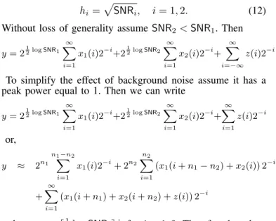
Pictorially the deterministic model is shown in Figure 2 (a).

In this particular examplen1= 5 andn2= 2, therefore both users receive the two most significant bits of the transmitted signal. However user 1 (strong user) receives three additional bits from the next three signal levels of the transmitted signal.

There is also the same correspondence betweennand channel gains in dB:

ni↔ d1

2logSNR_ie⁺, i= 1,2. (10) To analytically demonstrate how closely we are modeling the Gaussian BC channel, the capacity region of the Gaussian BC channel and the deterministic BC channel are shown in Figure 2 (b). As it is seen their capacity regions are very close to each other. In fact it is easy to verify that for all SNR’s these regions are always within one bit per user of each other, that is, if (R1, R2) is in the capacity region of the deterministic

BC then there is a rate pair within one bit component-wise of (R1, R2) that is in the capacity region of the Gaussian BC.

However, this is only the worst-case gap and in the typical case where SNR₁ and SNR₂ are very different, the gap is much smaller than one bit.

C. Modeling superposition

Consider a superposition scenario in which two users are simultaneously transmitting to a node. In the Gaussian model the received signal can be written as

y=h1x1+h2x2+z. (11) To intuitively see what happens in superposition in the Gaus- sian model, we again write the received signal,y, in terms of the binary expansions ofx1,x2 andz. Assumex1,x2 andz are all positive real numbers smaller than one, and also the channel gains are

hi=p

SNR_i, i= 1,2. (12) Without loss of generality assumeSNR₂<SNR₁. Then y= 2¹²^log^SNR¹

∞

X

i=1

x1(i)2⁻ⁱ+2¹²^log^SNR²

∞

X

i=1

x2(i)2⁻ⁱ+

∞

X

i=−∞

z(i)2⁻ⁱ. To simplify the effect of background noise assume it has a peak power equal to 1. Then we can write

y= 2¹²^log^SNR¹ X∞ i=1

x1(i)2⁻ⁱ+2¹²^log^SNR² X∞ i=1

x2(i)2⁻ⁱ+ X∞ i=1

z(i)2⁻ⁱ

or, y ≈ 2ⁿ¹

n1−n2

X

i=1

x1(i)2⁻ⁱ+ 2ⁿ²

n2

X

i=1

(x1(i+n1−n2) +x2(i)) 2⁻ⁱ

+ X∞ i=1

(x1(i+n1) +x2(i+n2) +z(i)) 2⁻ⁱ

whereni =d¹2logSNR_ie⁺ for i= 1,2. Therefore based on the intuition obtained from the point-to-point and broadcast AWGN channels, we can approximately model this as the following:

• That part of x1 that is above SNR2 (x1(i), 1 ≤ i ≤ n1−n2) is received clearly without any contribution from x2.

• The remaining part ofx1that is above noise level (x1(i), n1−n2< i≤n1) and that part ofx2that is above noise level (x1(i), 1 ≤i≤n2) are superposed on each other and are received without any noise.

• Those parts of x1 andx2 that are below noise level are truncated and not received at all.

The key point is how to model the superposition of the bits that are received at the same signal level. In our deterministic model we ignore the carry-overs of the real addition and we model the superposition by the modulo 2 sum of the bits that are arrived at the same signal level. Pictorially the deterministic model is shown in Figure 4 (a). Analogous to the deterministic model for the point-to-point channel, as seen in Figure 3, we can write

y=S^q⁻ⁿ¹x₁⊕S^q⁻ⁿ²x₂ (13)

(5)

9

Rx 2 Tx

Rx 1 n1

n2

(a) Pictorial representation of the deterministic model for Gaussian BC

n1 R2

R1 n2

1

2log(1 +SNR2)

1

2log(1 +SNR1)

(b) Capacity region of Gaussian BC (solid line) and deterministic BC (dashed line).

Fig. 2. Pictorial representation of the deterministic model for Gaussian BC is shown in (a). Capacity region of Gaussian and deterministic BC are shown in (b).

levels in the deterministic model represent the cloud center that is decoded by both users, and the remaining n

1

− n

2

levels represent the cloud detail that is decoded only by the strong user (after decoding the cloud center and canceling it from the received signal).

Pictorially the deterministic model is shown in Figure 2 (a). In this particular example n

1

= 5 and n

2

= 2, therefore both users receive the two most significant bits of the transmitted signal.

However user 1 (strong user) receives three additional bits from the next three signal levels of the transmitted signal. There is also the same correspondence between n and channel gains in dB:

n

i

↔ # 1

2 log SNR

i

$

⁺

, i = 1, 2. (10) To analytically demonstrate how closely we are modeling the Gaussian BC channel, the capacity region of the Gaussian BC channel and the deterministic BC channel are shown in Figure 2 (b). As it is seen their capacity regions are very close to each other. In fact it is easy to verify that for all SNR’s these regions are always within one bit per user of each other, that is, if (R

1

, R

2

) is in the capacity region of the deterministic BC then there is a rate pair within one bit component-wise of (R

1

, R

2

) that is in the capacity region of the Gaussian BC. However, this is only the worst-case gap and in the typical case where SNR

₁

and SNR

₂

are very different, the gap is much smaller than one bit.

(a) Pictorial representation of the deterministic model for Gaussian BC

Rx 2 Tx

Rx 1 n1

n2

(a) Pictorial representation of the deterministic model for Gaussian BC

n1 R2

R1 n2

1

2log(1 +SNR2)

1

2log(1 +SNR1)

levels in the deterministic model represent the cloud center that is decoded by both users, and the remaining n

1

− n

2

levels represent the cloud detail that is decoded only by the strong user (after decoding the cloud center and canceling it from the received signal).

Pictorially the deterministic model is shown in Figure 2 (a). In this particular example n

1

= 5 and n

2

= 2, therefore both users receive the two most significant bits of the transmitted signal.

However user 1 (strong user) receives three additional bits from the next three signal levels of the transmitted signal. There is also the same correspondence between n and channel gains in dB:

n

i

↔ # 1

2 log SNR

i

$

⁺

, i = 1, 2. (10) To analytically demonstrate how closely we are modeling the Gaussian BC channel, the capacity region of the Gaussian BC channel and the deterministic BC channel are shown in Figure 2 (b). As it is seen their capacity regions are very close to each other. In fact it is easy to verify that for all SNR’s these regions are always within one bit per user of each other, that is, if (R

1

, R

2

) is in the capacity region of the deterministic BC then there is a rate pair within one bit component-wise of (R

1

, R

2

) that is in the capacity region of the Gaussian BC. However, this is only the worst-case gap and in the typical case where SNR

₁

and SNR

₂

are very different, the gap is much smaller than one bit.

where the summation is inF² (modulo 2). Here xi(i= 1,2) andyare binary vectors of lengthqdenoting transmitted and received signals respectively andSis aq×qshift matrix. The relationship between ni’s and the channel gains is the same as in Equation (10).

11

model the superposition by the modulo 2 sum of the bits that are arrived at the same signal level. Pictorially the deterministic model is shown in Figure 4 (a). Analogous to the deterministic model for the point-to-point channel, as seen in Figure 3, we can write

y = S

^q⁻ⁿ¹

x

₁

⊕ S

^q⁻ⁿ²

x

₂

(16) where the summation is in F

²

(modulo 2). Here x

i

(i = 1, 2) and y are binary vectors of length q denoting transmitted and received signals respectively and S is a q × q shift matrix. The relationship between n

i

’s and the channel gains is the same as in Equation (10).

A

B

y1 D

y2

y3

y4

y5

x2(5) x2(3) x2(2) x2(4) x1(2) x1(3) x1(4) x1(5)

x2(1) x1(1)

Fig. 3. Algebraic representation of shift matrix deterministic model.

Compared to the point-to-point case we now have interaction between the bits that are received at the same signal level at the receiver. We limit the receiver to observe only the modulo 2 summation of those bits that arrive at the same signal level. This way of modeling signal interaction has two advantages over the simplistic collision model. First, if two bits arrive simultaneously at the same signal level, they are not both dropped and the receiver gets their modulo 2 summation. Second, unlike in the collision model where the entire packet is lost when there is collision, the most signi ficant bits of the stronger user remain intact. This is reminiscent of the familiar capture phenomenon in CDMA systems: the strongest user can be heard even when multiple users simultaneously transmit.

Now we can apply this model to the Gaussian MAC, in which

y = h

1

x

1

+ h

2

x

2

+ z (17)

Fig. 3. Algebraic representation of shift matrix deterministic model.

Compared to the point-to-point case we now have interaction between the bits that are received at the same signal level at the receiver. We limit the receiver to observe only the modulo 2 summation of those bits that arrive at the same signal level. This way of modeling signal interaction has two advantages over the simplistic collision model. First, if two bits arrive simultaneously at the same signal level, they are not both dropped and the receiver gets their modulo 2 summation.

Second, unlike in the collision model where the entire packet is lost when there is collision, the most significant bits of the stronger user remain intact. This is reminiscent of the familiar capturephenomenon in CDMA systems: the strongest user can be heard even when multiple users simultaneously transmit.

Now we can apply this model to the Gaussian MAC, in which

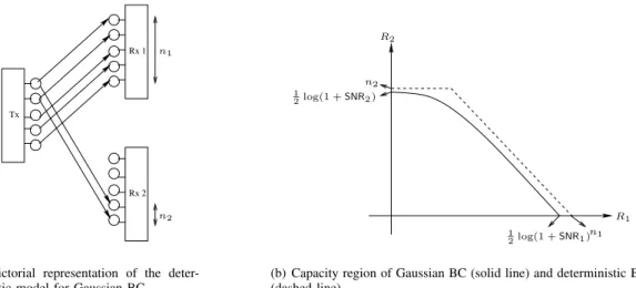
y=h1x1+h2x2+z (14) wherez∼ CN(0,1). There is also an average power constraint equal to 1 at both transmitters. A natural question is how close is the capacity region of the deterministic model to that of the actual Gaussian model. AssumeSNR₂<SNR₁. The capacity region of this channel is known to be the set of non-negative pairs(R1, R2)satisfying

Ri ≤ log(1 +SNR_i), i= 1,2 (15) R1+R2 ≤ log(1 +SNR₁+SNR₂). (16) This region is plotted with solid line in Figure 4 (b).

It is easy to verify that the capacity region of the deterministic MAC is the set of non-negative pairs(R1, R2)satisfying

R2 ≤ n2 (17)

R1+R2 ≤ n1 (18)

whereni =dlogSNRie⁺ for i = 1,2. This region is plotted with dashed line in Figure 4 (b). In this deterministic model the “carry-over” from one level to the next that would happen with real addition is ignored. However as we notice still the capacity region is very close to the capacity region of the Gaussian model. In fact it is easy to verify that they are within one bit per user of each other. The intuitive explanation for this is that in real addition once two bounded signals are added together the magnitude can become as large as twice the larger of the two signals. Therefore the number of bits in the sum is increased by at most one bit. On the other hand in finite-field addition there is no magnitude associated with signals and the summation is still in the same field as the individual signals.

So the gap between Gaussian and deterministic model for two user MAC is intuitively this one bit of cardinality increase.

Similar to the broadcast example, this is only the worst case gap and when the channel gains are different it is much smaller than one bit.

(6)

12

Tx 2

Rx Tx 1

n2 n1

(a) Pictorial representation of the deterministic MAC.

1

2log(1 +SNR1) R2

R1 1

2log(1 +SNR2) n2

n1

(b) Capacity region of Gaussian MAC (solid line) and deterministic MAC (dashed line).

Fig. 4. Pictorial representation of the deterministic MAC is shown in (a). Capacity region of Gaussian and deterministic MACs are shown in (b).

where z ∼ CN (0, 1). There is also an average power constraint equal to 1 at both transmitters.

A natural question is how close is the capacity region of the deterministic model to that of the actual Gaussian model. Assume SNR

2

< SNR

1

. The capacity region of this channel is known to be the set of non-negative pairs (R

1

, R

2

) satisfying

R

i

≤ log(1 + SNR

_i

), i = 1, 2 (18) R

1

+ R

2

≤ log(1 + SNR

₁

+ SNR

₂

). (19) This region is plotted with solid line in Figure 4 (b).

It is easy to verify that the capacity region of the deterministic MAC is the set of non-negative pairs (R

1

, R

2

) satisfying

R

2

≤ n

2

(20)

R

1

+ R

2

≤ n

1

(21)

where n

i

= # log SNR

i

$

⁺

for i = 1, 2. This region is plotted with dashed line in Figure 4 (b). In this deterministic model the “carry-over” from one level to the next that would happen with real addition is ignored. However as we notice still the capacity region is very close to the capacity region of the Gaussian model. In fact it is easy to verify that they are within one bit per user of each other. The intuitive explanation for this is that in real addition once two bounded signals are added together the magnitude can become as large as twice the larger of the two signals.

(a) Pictorial representation of the deterministic MAC.

12

Tx 2

Rx Tx 1

n2 n1

(a) Pictorial representation of the deterministic MAC.

1

2log(1 +SNR1) R2

R1 1

2log(1 +SNR2) n2

n1

where z ∼ CN (0, 1). There is also an average power constraint equal to 1 at both transmitters.

A natural question is how close is the capacity region of the deterministic model to that of the actual Gaussian model. Assume SNR

2

< SNR

1

. The capacity region of this channel is known to be the set of non-negative pairs (R

1

, R

2

) satisfying

R

i

≤ log(1 + SNR

_i

), i = 1, 2 (18) R

₁

+ R

₂

≤ log(1 + SNR

₁

+ SNR

₂

). (19) This region is plotted with solid line in Figure 4 (b).

It is easy to verify that the capacity region of the deterministic MAC is the set of non-negative pairs (R

1

, R

2

) satisfying

R

2

≤ n

2

(20)

R

1

+ R

2

≤ n

1

(21)

where n

i

= # log SNR

i

$

⁺

for i = 1, 2. This region is plotted with dashed line in Figure 4 (b). In this deterministic model the “carry-over” from one level to the next that would happen with real addition is ignored. However as we notice still the capacity region is very close to the capacity region of the Gaussian model. In fact it is easy to verify that they are within one bit per user of each other. The intuitive explanation for this is that in real addition once two bounded signals are added together the magnitude can become as large as twice the larger of the two signals.

Now we define the linear finite-field deterministic model for the relay network.

D. Linear finite-field deterministic model

The relay network is defined using a set of vertices V. The communication link from nodeito nodejhas a non-negative integer gain nij associated with it. This number models the channel gain in the corresponding Gaussian setting. At each time t, node i transmits a vector x_i[t] ∈ F^qp and receives a vectory_i[t]∈F^qpwhereq= maxi,j(n(ij))andpis a positive integer indicating the field size. The received signal at each node is a deterministic function of the transmitted signals at the other nodes, with the following input-output relation: if the nodes in the network transmit x₁[t],x₂[t], . . .x_N[t] then the received signal at node j, 1≤j≤N is:

yj[t] =X

S^q⁻ⁿ^ijxi[t] (19) where the summations and the multiplications are in F^p. Throughout this paper the field size, p, is assumed to be 2, unless it is stated otherwise.

E. Limitation: Modeling MIMO

The examples in the previous subsections may give the impression that the capacity of any Gaussian channel is within a constant gap to that of the corresponding linear deterministic model. The following example shows that is not the case.

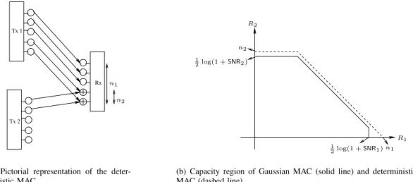
Consider a2×2MIMO real Gaussian channel with channel gain values as shown in Figure 5 (a), where k is an integer larger than 2. The channel matrix is

H= 2^k ₃

4 1 1 1

. (20)

The channel gain parameters of the corresponding linear finite- field deterministic model are:

n11 = d1

2log₂|h11|²e⁺=dlog₂(2^k−2^k−2)e⁺=k n12 = n21=n22=dlog₂2^ke⁺=k (21)

14

2^k−2^k−2

2^k 2^k 2^k Tx1

Tx2

Rx1

Rx2 (a)

k Tx1 Rx1

Tx2 Rx2

(b)

Fig. 5. An example of a2×2Gaussian MIMO channel is shown in(a). The corresponding linearfinite-field deterministic MIMO channel is shown in(b).

The channel gain parameters of the corresponding linearfinite-field deterministic model are:

n11 = "1

2log2|h11|²#⁺="log2(2^k−2^k−2)#⁺=k (24)

n12 = n21=n22="log22^k#⁺=k (25)

Now let us compare the capacity of the MIMO channel under these two models for large values ofk. For the Gaussian model, both singular values ofHare of the order of2^k. Hence, the capacity of the real Gaussian MIMO channel is of the order of

2×1

2log(1 +|2^k|²)≈2k.

However the capacity of the corresponding linearfinite-field deterministic MIMO is simply

CLFF = rank



Ik Ik

Ik Ik



=k. (26)

Hence the gap between the two capacities goes to infinity askincreases.

Even though the linear deterministic channel model does not approximate the Gaussian channel in all scenarios, it is still useful in providing insights in many cases, as will be seen in the next section. Moreover, its analytic simplicity allows an exact analysis of the relay network capacity.

This in turns provides the foundation for the analysis of the Gaussian network.

(a)

14

2^k−2^k−2

2^k 2^k 2^k Tx1

Tx2

Rx1

Rx2 (a)

k Tx1 Rx1

Tx2 Rx2

(b)

Fig. 5. An example of a2×2Gaussian MIMO channel is shown in(a). The corresponding linearfinite-field deterministic MIMO channel is shown in(b).

The channel gain parameters of the corresponding linearfinite-field deterministic model are:

n11 = "1

2log2|h11|²#⁺="log2(2^k−2^k−2)#⁺=k (24)

n12 = n21=n22="log22^k#⁺=k (25)

Now let us compare the capacity of the MIMO channel under these two models for large values ofk. For the Gaussian model, both singular values ofHare of the order of2^k. Hence, the capacity of the real Gaussian MIMO channel is of the order of

2×1

2log(1 +|2^k|²)≈2k.

However the capacity of the corresponding linearfinite-field deterministic MIMO is simply

CLFF = rank



Ik Ik

Ik Ik



=k. (26)

Hence the gap between the two capacities goes to infinity askincreases.

Even though the linear deterministic channel model does not approximate the Gaussian channel in all scenarios, it is still useful in providing insights in many cases, as will be seen in the next section. Moreover, its analytic simplicity allows an exact analysis of the relay network capacity.

This in turns provides the foundation for the analysis of the Gaussian network.

(b)

Fig. 5. An example of a2×2Gaussian MIMO channel is shown in(a).

The corresponding linear finite-field deterministic MIMO channel is shown in(b).

Now let us compare the capacity of the MIMO channel under these two models for large values of k. For the Gaussian model, both singular values ofHare of the order of2^k. Hence, the capacity of the real Gaussian MIMO channel is of the order of

2×1

2log(1 +|2^k|²)≈2k.

However the capacity of the corresponding linear finite-field deterministic MIMO is simply

CLFF = rank

Ik Ik

=k. (22)

Hence the gap between the two capacities goes to infinity as kincreases.

Even though the linear deterministic channel model does not approximate the Gaussian channel in all scenarios, it is still useful in providing insights in many cases, as will be seen in the next section. Moreover, its analytic simplicity allows an exact analysis of the relay network capacity. This in turns provides the foundation for the analysis of the Gaussian network.

(7)

7

16

S D

R hRD hSR

hSD (a) The Gaussian relay channel

R

S

nSD D

nSR nRD

(b) The linearfinite-field deterministic relay channel Fig. 6. The relay channel: (a) Gaussian model, (b) Linearfinite-field deterministic model.

!!"

!#"

!$"

"

$"

#"

!"

!!"

!#"

!$"

"

$"

#"

!"

"

"%&

$

'(_)*'^#+'(_,*'^#

'(_,)'^#+'(_,*'^#

-./

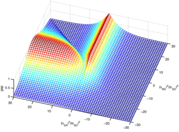
Fig. 7. The x and y axis respectively represent the channel gains from relay to destination and source to relay normalized by the gain of the direct link (source to destination) in dB scale. The z axis shows the value of the gap between the cut-set upper bound and the achievable rate of decode-forward scheme in bits/sec/Hz.

of bits that the source can broadcast, and the maximum number of bits that the destination can receive. Therefore

C^d_relay ≤ min (max(nSR, nSD),max(nRD, nSD)) (28)

=





nSD, ifnSD>min (nSR, nRD);

min (nSR, nRD), otherwise. (29)

(a) The Gaussian relay channel

16

S D

R hRD hSR

hSD (a) The Gaussian relay channel

R

S

nSD D

nSR nRD

!!"

!#"

!$"

"

$"

#"

!"

!!"

!#"

!$"

"

$"

#"

!"

"

"%&

$

'(_)*'^#+'(_,*'^#

'(_,)'^#+'(_,*'^#

-./

Crelay^d ≤ min (max(nSR, nSD),max(nRD, nSD)) (28)

=





(b) The linear finite-field deterministic relay channel

Fig. 6. The relay channel: (a) Gaussian model, (b) Linear finite-field deterministic model.

III. MOTIVATION OF OUR APPROACH

In this section we motivate and illustrate our approach. We look at three simple relay networks and illustrate how the analysis of these networks under the simpler linear finite-field deterministic model enables us to conjecture an approximately optimal relaying scheme for the Gaussian case. We progress from the relay channel where several strategies yield uniform approximation to more complicated networks where progressively we see that several “simple” strategies in the literature fail to achieve a constant gap. Using the deterministic model we can whittle down the potentially successful strategies. This illustrates the power of the deterministic model to provide insights into transmission techniques for noisy networks.

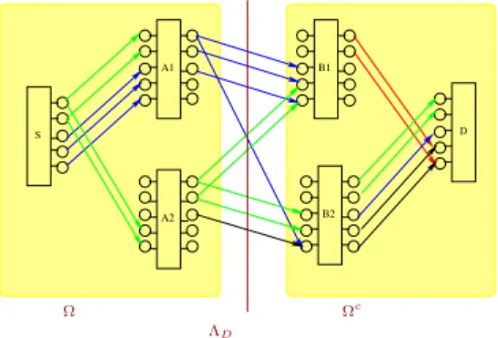
The network is assumed to be synchronized, i.e.,all transmissions occur on a common clock. The relays are allowed to do any causal processing. Therefore their current output depends only its past received signals. For any such network, there is a natural information-theoretic cut-set bound [19], which upper bounds the reliable transmission rateR. Applied to the relay network, we have the cut-set upper bound C on its capacity:

C= max

p({xj}j∈V) min

Ω∈ΛD

I(y_Ω^c;xΩ|xΩ^c) (23) where ΛD ={Ω :S ∈Ω, D∈ Ω^c} is all source-destination cuts. In words, the value of a given cut Ωis the information rate achieved when the nodes in Ωfully cooperate to transmit and the nodes in Ω^c fully cooperate to receive. In the case of Gaussian networks, this is simply the mutual information achieved in a MIMO channel, the computation of which is standard. We will use this cut-set bound to assess how good our achievable strategies are.

A. Single-relay network

We start by looking at the simplest Gaussian relay network with only one relay as shown in Figure 6 (a). To approximate its capacity uniformly (uniform over all channel gains), we need to find a relaying protocol that achieves a rate close to

S D

R

hRD

hSR

hSD

(a) The Gaussian relay channel

R

S

nSD D

nSR nRD

!!"

!#"

!$"

"

$"

#"

!"

!!"

!#"

!$"

"

$"

#"

!"

"

"%&

$

'(_)*'^#+'(_,*'^#

'(_,)'^#+'(_,*'^#

-./

C_relay^d ≤ min (max(nSR, nSD),max(nRD, nSD)) (28)

=





an upper bound on the capacity for all channel parameters. To find such a scheme we use the linear finite-field deterministic model to gain insight. The corresponding linear finite-field deterministic model of this relay channel with channel gains denoted by nSR, nSD and nRD is shown in Figure 6 (b).

It is easy to see that the capacity of this deterministic relay channel,C_relay^d , is smaller than both the maximum number of bits that the source can broadcast, and the maximum number of bits that the destination can receive. Therefore

C_relay^d ≤min (max(nSR, nSD),max(nRD, nSD))

=

min (nSR, nRD), otherwise.

(24) It is not difficult to see that this is in fact the cut-set upper bound for the linear deterministic network.

Note that Equation (24) naturally implies a capacity- achieving scheme for this deterministic relay network: if the direct link is better than any of the links to/from the relay then the relay is silent, otherwise it helps the source by decoding its message and sending innovations. In the example of Figure 6, the destination receives two bits directly from the source, and the relay increases the capacity by 1 bit by forwarding the least significant bit it receives on a level that does not overlap with the direct transmission at the destination.

This suggests a decode-and-forward scheme for the original Gaussian relay channel. The question is: how does it perform?

Although unlike in the deterministic network, the decode- forward protocol cannot achieve exactly the cut-set bound in the Gaussian nettwork, the following theorem shows it is close.

Theorem 3.1: The decode-and-forward relaying protocol achieves within 1 bit/s/Hz of the cut-set bound of the single- relay Gaussian network, for all channel gains.

Proof:See Appendix A.

We should point out that even this 1-bit gap is too conserva- tive for many parameter values. In fact the gap would be at the maximum value only if two of the channel gains are exactly