Softwarepraktikum (Wissenschaftliches Rechnen) f¨ur Fortgeschrittene

(1)

Softwarepraktikum

(Wissenschaftliches Rechnen) f¨ ur Fortgeschrittene

Pavel Hron, Arsalan Farooq Ruprecht-Karls-Universit¨at Heidelberg

Interdisziplin¨ares Zentrum f¨ur Wissenschaftliches Rechnen email: paja.hron@email.cz

February 12, 2010

(2)

1 Problem Formulation

Consider the steady-state groundwater flow equation (General Diffusion Equation) with corre- sponding Dirichlet and Neumann boundary conditions

−∇ · {K(x)∇p}=f in Ω⊆Rⁿ, n= 2,3, (1a)

p=g on ΓD ⊆∂Ω, (1b)

−(∇ ·K(x)∇p)·n(x) =j on Γ_N =∂Ω\Γ_D 6=∂Ω, (1c) whereK is the absolute permeability.

K :Rⁿ−→Rⁿ^×ⁿ is a projection, which relates to each pointx ∈Ω an×n matrixK(x). We demand also (for all x∈ Ω) thatK(x)

1. K(x) =K^T(x) andξ^TK(x)ξ >0 ∀ξ∈Rⁿ, ξ6= 0 (symmetric positive definite), 2. C(x) := min{ξ^TK(x)ξ| kξk= 1} ≥C0>0 (uniform ellipticity).

In this problem we assume that permeabilityK is strongly varying in the domain Ω.

Denote the volumetric flux function through a porous mediumJ~

J~(x) =−K(x)∇p. (2)

We want to solve the equation (1) in Ω = [0,1]^d, without sink or source therms (f = 0) and appropriate boundary conditions. On the left hand side and right hand side of the domain Ω is Dirichlet boundary condition with p = 1 andp = 0 respectively. The upper and the lower boundaries of Ω are impermeable, which means Neumann boundary condition is zero.

Above mentioned problem description we can write in the mathematical form

∇ ·J~(x) = 0 in Ω = [0,1]^d, d= 2,3, (3a)

p= 1 on ΓD1 ={x= (x¹, . . . , x_d)|x¹ = 0, x², . . . , x_d∈[0,1]} ⊆∂Ω, (3b) p= 0 on Γ_D2 ={x= (x1, . . . , x_d)|x1 = 1, x2, . . . , x_d∈[0,1]} ⊆∂Ω, (3c)

−∇p·n(x) = 0 on Γ_N =∂Ω\(Γ_D1∪Γ_D2)6=∂Ω. (3d)

The main goal of this project is to get the overall fluxF over the right face Γ_D2 of the domain Ω F =

Z

Γ_D

2

J~(x)·n(x)dl. (4)

At first we have to solve system (3). For this purpose we use following numerical methods:

• Cell Centered Finite Volumes (FV)

• Mixed Finite Elements (MFEM)

• Conforming Finite Elements (FEM)

• Odeon-Baumann-Babuska Discontinuous Galerkin (DG)

(3)

2 Flux implementation in DUNE

The DUNE (Distributed and Unified Numerics Environment, www.dune-project.org) consists of many modules. In the module dune-pdelab-howto above mentioned methods for problem (3) are already implemented. The objective of our work was the implementation of a function, which calculates the integral (4).

2.1 Cell Centered Finite Volumes

The result of (3) for CCFV method is function, which is constant on each grid cell. If we have conforming, structured rectangular (2D) or cuboid (3D) grid, the term ∇p·n(x) on the face can be approximated as

∇p·n(x) = p_l−p_r

d , (5)

where p_l,pr are the values of the pressure p in cells and dis the distance between centroids of this two cells. Then we can evaluate integral (4) using mid-point rule.

pl pr

d

File fluxfv.hh

1 template < typename GV , typename DGF , typename KType >

2 void flux ( const GV & gv , const DGF & dgf , const KType & k )

3 {

4 // f i r s t we e x t r a c t t h e di m e n s i on s o f t h e g r i d

5 const int dim = GV :: dimension ;

6 const int dimworld = GV :: d i m e n s i o n w o r l d ;

7 const double epsilon =1 e -10;

8

9 // d i s c r e t e g r i d f u n c t i o n r an g e t y p e

10 typename DGF :: Traits :: RangeType RT ;

11

12 // k i n s i d e t h e e l e m e n t

13 typename KType :: Traits :: RangeType k_inside ;

14

15 // t y p e u s e d f o r c o o r d i n a t e s i n t h e g r i d

16 typedef typename GV :: ctype ct ;

17

18 // e l e m e n t i t e r a t o r s

19 typedef typename GV :: template Codim <0 >:: Iterator E l e m e n t L e a f I t e r a t o r ;

20 typedef typename GV :: I n t e r s e c t i o n I t e r a t o r I n t e r s e c t i o n I t e r a t o r ;

21

22 // f l u x o v e r a l l

23 double flux_sum =0.0;

24 // l o o p ov e r e l e m e n t s

25 for ( E l e m e n t L e a f I t e r a t o r it = gv . template begin <0 >();

26 it != gv . template end <0 >(); ++ it )

27 {

28 // c e l l geometry t y p e

29 Dune :: G e o m e t r y T y p e gt = it - > type ();

30

31 // c e l l c e n t e r i n r e f e r e n c e e l e m e n t

32 const Dune :: FieldVector < ct , dim >& local = Dune :: Referenc eEl e me nt s < ct , dim >::

33 general ( gt ). position (0 ,0);

34

35 // c e l l c e n t e r i n g l o b a l c o o r d i n a t e s

(4)

37 global = it - > geometry (). global ( local );

38

39 // c e l l volume , assume l i n e a r map he r e

40 double volume = it - > geometry (). i n t e g r a t i o n E l e m e n t ( loca l )

41 * Dune :: ReferenceEl em en t s < ct , dim >:: general ( gt ). volum e ();

42

43 // run t h r o u g h a l l i n t e r s e c t i o n s w i t h n e i g h b o r s and boundary

44 I n t e r s e c t i o n I t e r a t o r isend = gv . iend (* it );

45 for ( I n t e r s e c t i o n I t e r a t o r is = gv . ibegin (* it ); is != isend ; ++ is )

46 {

47 // g e t geometry t y p e o f f a c e

48 Dune :: G e o m e t r y T y p e gtf = is - > type ();

49

50 // c e n t e r i n f a c e ’ s r e f e r e n c e e l e m e n t

51 const Dune :: FieldVector < ct , dim -1 >&

52 facelocal = Dune :: ReferenceEl em e nt s < ct , dim -1 >:: genera l ( gtf ). position (0 ,0);

53

54 // c e l l c e n t e r i n g l o b a l c o o r d i n a t e s

55 Dune :: FieldVector < ct , dimworld >

56 faceglobal = is - > geometry (). global ( facelocal );

57

58 // f a c e volume

59 ct face_volum e = is - > i n t e r s e c t i o n G l o b a l (). volume ();

60

61 // d i s t a n c e : e l e m e n t c e n t e r t o f a c e c e n t e r

62 float d =0;

63 for ( size_t i =0; i < dim ; i ++)

64 {

65 d +=( faceglobal [ i ] - global [ i ])*( facegloba l [ i ] - global [ i ]);

66 }

67 d = sqrt ( d );

68

69 // f l u x e v a l u a t i o n

70 if ( fabs ( faceglobal [0] -1.0) < epsilon )

71 {

72 dgf . evaluate (*( it ) , local , RT );

73 k . evaluate (*( it ) , local , k_inside );

74 flux_sum += face_volum e * k_inside * RT / d ;

75 }

76 }

77 }

78 std :: cout << " flux overall " << flux_sum << std :: endl ;

79 80 }

2.2 Mixed Finite Elements

If we use MFEM method, we gain not only pressurep, but also the termJ~(x). That is why the calculation of integral (4) is easy.

1 template < typename GV , typename RT0DGF >

2 void flux ( const GV & gv , const RT0DGF & rt0dgf )

3 {

5 double epsilon =1 e -10;

6

9 const int dimworld = GV :: d i m e n s i o n w o r l d ;

10

11 typename RT0DGF :: Traits :: RangeType RT ;

12 typedef typename RT0DGF :: Traits :: D o m a i n F i e l d T y p e DF ;

13 typedef typename RT0DGF :: Traits :: R a n g e F i e l d T y p e RF ;

14 15

(5)

20

21 // l o o p ov e r e l e m e n t s

24 {

27

29 const Dune :: FieldVector < ct , dim >&

30 local = Dune :: ReferenceEle m en ts < ct , dim >:: general ( gt ). position (0 ,0);

31

35 {

38

41 facelocal = Dune :: ReferenceEl em e nt s < ct , dim -1 >:: genera l ( gtf ). position (0 ,0);

42

43 // c e n t e r o f f a c e i n g l o b a l c o o r d i n a t e s

44 Dune :: FieldVector < ct , dimworld > faceglobal = is - > geomet ry (). global ( facelocal );

45 46

47 // i s t h e x−c o o r d i n a t e s o f f a c e c e n t e r = 1

49 {

50 // g e t normal v e c t o r s c a l e d w i t h volume

51 Dune :: FieldVector < ct , dimworld > i n t e g r a t i o n O u t e r N o r m a l =

52 is - > i n t e g r a t i o n O u t e r N o r m a l ( facelocal );

53 i n t e g r a t i o n O u t e r N o r m a l *=

54 Dune :: ReferenceEl em en t s < ct , dim -1 >:: general ( gtf ). vol ume ();

55

56 // l o o p ov e r q u a d r a t u r e r u l e s , o r d e r=1

57 const Dune :: QuadratureRule < DF , dim -1 >& rule =

58 Dune :: QuadratureRul es < DF , dim -1 >:: rule ( gtf ,1);

59 for ( typename Dune :: QuadratureRule < DF , dim -1 >:: c o n s t _ i t e r a t o r cit =

60 rule . begin (); cit != rule . end (); ++ cit )

61 {

62 // p o s i t i o n o f q u a d r a t u r e p o i n t i n l o c a l c o o r d i n a t e s o f e l e me n t

63 Dune :: FieldVector < DF , dim > local =

64 is - > g e o m e t r y I n I n s i d e (). global ( cit - > position ());

65 RF factor = cit - > weight ();

66

67 // k∗v e l o c i t y e v a l u a t i o n

68 rt0dgf . evaluate (* it , local , RT );

69

70 flux_sum += i n t e g r a t i o n O u t e r N o r m a l * RT * factor ;

71

72 } // c i t

73

74 } // b o r d e r

75

76 } // i s

77 } // i t

78 std :: cout << " flux overall " << flux_sum << std :: endl ;

79 }

(6)

2.3 Conforming Finite Elements, Discontinuous Galerkin

The solution p(x) of problem (3) can be expressed as p(x) =X

ei

n_ei

X

j=1

c_ei,j·ψ_ei,j(x). (6)

For each element e_i there is a set of base functions ψ_ei,j(x), which are multiplicated with coefficients c_ei,j. Therefore∇p we get as

∇p(x) =X

eⁱ n_ei

X

j=1

c_ei,j· ∇ψei,j(x). (7) For evaluation of integral (4) we can use again numerical integration.

1 template < typename GV , typename X , typename GFS , typename KType >

2 void flux ( const GV & gv , const X & x , const GFS & gfs , const KTyp e & k , int intorder =1)

3 {

4

6 double epsilon =1 e -10;

7

10 const int dimw = GV :: d i m e n s i o n w o r l d ;

11

12 typedef typename GFS :: L o c a l F u n c t i o n S p a c e :: Traits :: L o c a l F i n i t e E l e m e n t T y p e ::

13 Traits :: L o c a l B a s i s T y p e :: Traits :: D o m a i n F i e l d T y p e DF ;

15 Traits :: L o c a l B a s i s T y p e :: Traits :: R a n g e F i e l d T y p e RF ;

17 Traits :: L o c a l B a s i s T y p e :: Traits :: J a c o b i a n T y p e J a c o b i a n T y p e ;

18

19 typedef typename GFS :: L o c a l F u n c t i o n S p a c e LFS ;

20 LFS lfs ( gfs ); // l o c a l f u n c t i o n s p a c e l

21

22 std :: vector < RF > xl ; // l o c a l c o n t a i n e r

23 typename KType :: Traits :: RangeType k_inside ; // K t e n s o r

24 25

28

31

34 {

37

39 const Dune :: FieldVector < ct , dim >&

40 local = Dune :: ReferenceEle m en ts < ct , dim >:: general ( gt ). position (0 ,0);

41

42 // e v a l u a t e k t e n s o r

43 k . evaluate (*( it ) , local , k_inside );

44

48 {

(7)

51

54 facelocal = Dune :: ReferenceEle me n ts < ct , dim -1 >:: genera l ( gtf ). position (0 ,0);

55

56 // g e t normal v e c t o r s c a l e d w i t h volume

57 Dune :: FieldVector < ct , dimw > i n t e g r a t i o n O u t e r N o r m a l

58 = is - > i n t e g r a t i o n O u t e r N o r m a l ( facelocal );

59 i n t e g r a t i o n O u t e r N o r m a l

60 *= Dune :: ReferenceEl em e nt s < ct , dim -1 >:: general ( gtf ). v olume ();

61

62 // c e n t e r o f f a c e i n g l o b a l c o o r d i n a t e s

63 Dune :: FieldVector < ct , dimw > faceglobal = is - > geometry (). global ( facelocal );

64

66 {

67 // l o o p ov e r q u a d r a t u r e p o i n t s

68 const Dune :: QuadratureRule < DF , dim -1 >& rule =

69 Dune :: QuadratureRul es < DF , dim -1 >:: rule ( gtf , intorder );

70 for ( typename Dune :: QuadratureRule < DF , dim -1 >:: c o n s t _ i t e r a t o r

71 cit = rule . begin (); cit != rule . end (); ++ cit )

72 {

73

74 // p o s i t i o n o f q u a d r a t u r e p o i n t i n l o c a l c o o r d i n a t e s o f e l e me n t

75 Dune :: FieldVector < DF , dim > local =

76 is - > g e o m e t r y I n I n s i d e (). global ( cit - > position ());

77

78 RF factor = cit - > weight ();

79

80 lfs . bind (* it );

81 lfs . vread (x , xl ); // w r i t e l o c a l c o n t a i n e r i n t o x l

82

83 // e v a l u a t e j a c o b i a n

84 std :: vector < JacobianType > js ( lfs . size ());

85 lfs . l o c a l F i n i t e E l e m e n t (). localBasis (). e v a l u a t e J a c o b i a n ( local , js );

86

87 // t r a n s f o r m g r a d i e n t t o r e a l e l e m e n t

88 const Dune :: FieldMatrix < DF , dimw , dim > jac =

89 it - > geometry (). j a c o b i a n I n v e r s e T r a n s p o s e d ( local );

90 std :: vector < Dune :: FieldVector < RF , dim > > gradphi ( lfs . s ize ());

91 for ( size_t i =0; i < lfs . size (); i ++)

92 {

93 gradphi [ i ] = 0.0;

94 jac . umv ( js [ i ][0] , gradphi [ i ]);

95 }

96

97 // compute g r a d i e n t o f u

98 Dune :: FieldVector < RF , dim > gradu (0.0);

99 for ( size_t i =0; i < lfs . size (); i ++)

100 gradu . axpy ( xl [ i ] , gradphi [ i ]);

101

102 // compute K ∗ g r a d i e n t o f u

103 Dune :: FieldVector < RF , dim > Kgradu (0.0);

104 k_inside . umv ( gradu , Kgradu );

105 flux_sum += i n t e g r a t i o n O u t e r N o r m a l * Kgradu * factor ;

106

107 } // c i t

108

109 } // b o r d e r

110

111 } // i s

112 } // i t

113

114 std :: cout << " flux overall " << -1* flux_sum << std :: endl ;

115 116 }

(8)

3 Numerical results

In this chapter we will discuss some numerical results for different permeability fields. This examples shows, that the cell-centered Finite Volume Method, Discontinuous Galerkin Method and Mixed Finite Elements Method tend to underestimate the overall flux, the Finite Ele- ment Method tend to overestimate the overall flux. Finite Element Method converges only for continuous permeability fields.

3.1 Durlofsky permeability field

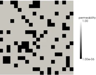
Durlofsky has defined the permeabillity field on a regular 20×20 mesh (see Fig. 1). The permeability in dark areas isK = 10⁻⁶, in light areas isK= 1.

The unit square is discretized with 20×20 rectangular elements for cube grid or with 20×20×2 triangular elements for simplex grid. Finer grids are obtained through regular refinement.

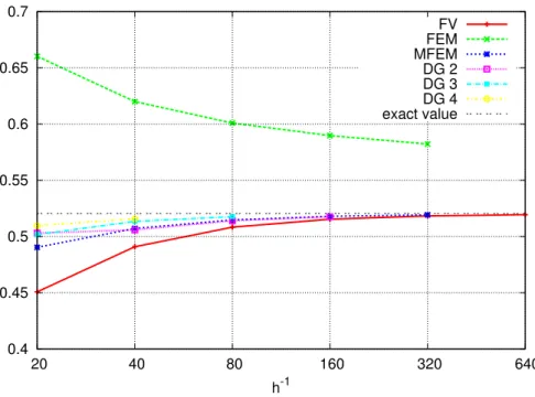
The exact value ofF for Durlofsky permeability field¹ has been given in as 0.5205. In Table 1 and in Fig. 2 we show results for the unknown overall flux through the systemF with rectangle grid discretization. We compare above mentioned numerical schemes. The results clearly show the unsuitability of the Conforming Finite Element Method for this type of problem, because this method has a bad approximation of average permeability.

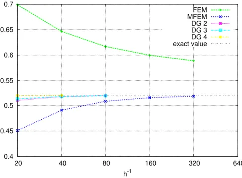
For rectangular grid we get good results with the lowest order Mixed Finite Element Method.

Discontinuous Galerkin Method gives the best results, this method is locally mass conservative and in comparison with Finite Volume Method uses more degrees of freedom. The result for triangular grid discretization are shown in Fig. 3 and in Table 2. In this case Mixed Finite Element Method is worse than rectangle grid discretization.

Figure 1: Durlofsky permeability field.

1L. J. Durlofsky,Accuracy of mixed and control volume finite element approximations to Darcy velocity and related quantities, Water Resources Reserach30(1994), no. 4, 965-973

(9)

h^-1

FV FEM MFEM DG 2 DG 3 DG 4 exact value

0.4 0.45 0.5 0.55 0.6 0.65 0.7

20 40 80 160 320 640

Figure 2: The overall fluxF for the Durlovsky problem calculated with diferent discretization schemes and successive grid refinement, rectangle grid discretization.

h⁻¹ FV MFEM DG, r=2 DG, r=3 DG, r=4 FEM,Q1

20 0.450829 0.490408 0.503091 0.501675 0.509603 0.660146 40 0.49096 0.507119 0.505838 0.513495 0.51577 0.619998 80 0.508343 0.514745 0.513997 0.517623 0.600907

160 0.515426 0.517945 0.517588 0.589748

320 0.518264 0.515426 0.582236

640 0.519393

Table 1: The overall fluxF for the Durlovsky problem, rectangles.

(10)

h^-1

FEM MFEM DG 2 DG 3 DG 4 exact value

0.4 0.45 0.5 0.55 0.6 0.65 0.7

20 40 80 160 320 640

Figure 3: The overall fluxF for the Durlovsky problem calculated with diferent discretization schemes and successive grid refinement, triangle grid discretization.

h⁻¹ MFEM FEM, P1 DG, r=2 DG, r=3 DG, r=4 20 0.450829 0.699048 0.510242 0.512905 0.519586 40 0.49096 0.646453 0.517507 0.517643 0.519838 80 0.508343 0.616949 0.519378 0.519183

160 0.515426 0.59974 320 0.518264 0.588928 640

Table 2: The overall fluxF for the Durlovsky problem, triangles.

(11)

3.2 Discontinuous permeability field

Durlofsky permeability field is discontinuous, it consists of only 2 values. The distribution is irregular. In this example we describe discontinuous permeability field with periodic distribution.

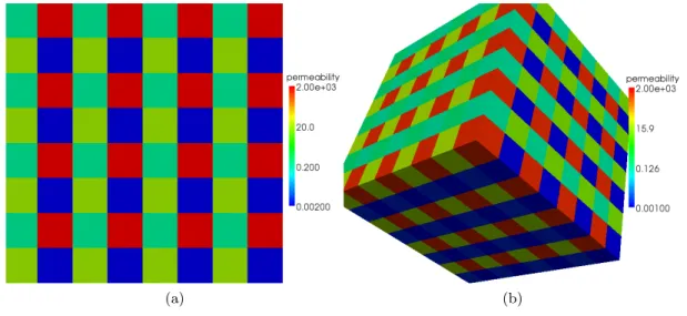
This discontinuous permeability field can be for all x= (x1, x2, x3)∈Ω defined by the formula

K(x) =











20.0 ⌊^x_h¹⌋ even,⌊^x_h²⌋even,⌊^x_h³⌋ even 0.002 ⌊^x_h¹⌋ odd,⌊^x_h²⌋ even,⌊^x_h³⌋ even 0.2 ⌊^x_h¹⌋ even,⌊^x_h²⌋odd,⌊^x_h³⌋ even 2000.0 ⌊^x_h¹⌋ odd,⌊^x_h²⌋ odd,⌊^x_h³⌋even 1000.0 ⌊^x_h¹⌋ even,⌊^x_h²⌋even,⌊^x_h³⌋ odd 0.001 ⌊^x_h¹⌋ odd,⌊^x_h²⌋ even,⌊^x_h³⌋ odd 0.1 ⌊^x_h¹⌋ even,⌊^x_h²⌋odd,⌊^x_h³⌋ odd 10.0 ⌊^x_h¹⌋ odd,⌊^x_h²⌋ odd,⌊^x_h³⌋odd

. (8)

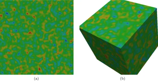
This permeability field in 2D and in 3D is shown in Figure 4.

The mesh size in this problem is taken as 16×16 to prevent the problem from complexity.

Table 3.2 and 3.2 show the results of the flux for different methods with successive refinements.

As in the case of Finite Element Method, we are not getting good results because this method has a bad approximation for permeability field and not locally mass conservative and secondly it is discrete and not smooth enough. Therefore, we are not including the fluxes for FEM in the graph.

(a) (b)

Figure 4: Discontinuous permeability field.

(12)

h^-1

FV MFEM DG 2 DG 3 DG 4

0.25 0.3 0.35 0.4 0.45 0.5 0.55 0.6 0.65 0.7 0.75 0.8

16 32 64 128 256

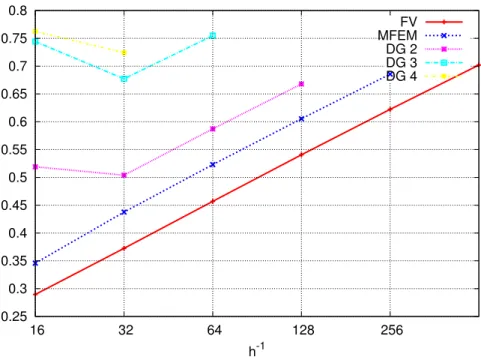
Figure 5: The overall flux F for the discontinuous permeability field (8) in 2D at successive refinements, rectangular grid discritization.

16 0.289657 0.345877 0.519077 0.74418 0.762491 11.6776 32 0.372477 0.437726 0.503865 0.677174 0.724126 9.22717 64 0.45705 0.522987 0.58715 0.754825 7.72284

128 0.540632 0.605493 0.667953 6.6705

256 0.622409 0.685629 5.89056

512 0.701939 5.29135

Table 3: The overall fluxF for the discontinuous permeability field (8) in 2D, rectangles.

(13)

h^-1

MFEM DG 2 DG 3 DG 4

0.2 0.3 0.4 0.5 0.6 0.7 0.8 0.9

16 32 64 128 256 512

Figure 6: The overall flux F for the discontinuous permeability field (8) in 2D at successive refinements, triangular grid discritization.

h⁻¹ MFEM DG, r=2 DG, r=3 DG, r=4 FEM,P1 16 0.289657 0.569913 0.600637 0.6859 14.2598 32 0.372476 0.652479 0.685519 0.766271 10.9272 64 0.457048 0.734066 0.764934 8.86621

128 0.540628 0.812042 7.48263

256 0.622395 6.49433

512 5.82135

Table 4: The overall fluxF for the discontinuous permeability field (8) in 2D, triangles.

h⁻¹ FV MFEM DG, r=2 FEM,Q1

16 0.163812 0.175001 0.296727 251.52 32 0.217076 0.259619 0.296727 94.7228

64 0.279882 48.9817

128 0.34436 27.0621

Table 5: The overall flux F for the discontinuous permeability field (8) in 3D, cuboids.

(14)

3.3 Random permeability field

The function K(x) is log-normal distributed with a given mean of 0, a variance of 3 (i.e. the permeabilities alternating between 10⁻³ and 10³) and a correlation length of 1/64 or 1/16 in 2D and 1/32 or 1/8 in 3D. Examples of these random permeability fields are shown in Fig. 7 and 8.

(a) (b)

Figure 7: Log-normal distributed permeability fields in 2D and 3D, correlation length of 1/64 in 2D and 1/32 in 3D.

(a) (b)

Figure 8: Log-normal distributed permeability fields in 2D and 3D, correlation length of 1/16 in 2D and 1/8 in 3D.

Numerical results for random permeability field with smaller correlation length (Fig. 9, 10 and Tab. 6, 7 and 8) shows, that all methods converge. The rate of convergence is smaller than the rate of convergence for random permeability field with greater correlation length (see Fig.

11, 12 and Tab. 9, 10 and 11). The reason is that random permeability field with greater correlation length is smoother. In this case FEM also converges, in contrast to discontinuous

(15)

h^-1

FV FEM MFEM DG 2 DG 3 DG 4

0.75 0.8 0.85 0.9 0.95 1 1.05 1.1 1.15 1.2 1.25

16 32 64 128 256 512

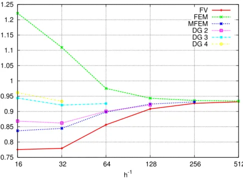
Figure 9: The overall flux F for the random permeability field 2D problem with correlation length of 1/64 calculated with diferent discretization schemes and successive grid refinement, rectangle grid discretization.

permeability field.

16 0.77534 0.836949 0.868496 0.943831 0.961535 1.22132 32 0.779322 0.84461 0.8621 0.920732 0.93326 1.1095

64 0.85643 0.898071 0.90065 0.9257423 0.975436

128 0.908352 0.924298 0.921081001 0.943341

256 0.926655 0.931132 0.935863

512 0.931683 0.934049

Table 6: The overall flux F for the random permeability 2D field with correlation length of 1/64, rectangles.

(16)

h^-1

FEM MFEM DG 2 DG 3 DG 4

0.6 0.8 1 1.2 1.4 1.6 1.8

16 32 64 128 256 512

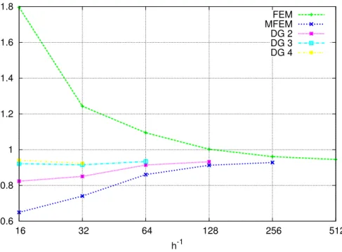
Figure 10: The overall flux F for the random permeability field 2D problem with correlation length of 1/64 calculated with diferent discretization schemes and successive grid refinement, triangle grid discretization.

128 0.912719 1.00245 0.932027 256 0.928019 0.960686

512 0.944735

Table 7: The overall flux F for the random permeability 2D field with correlation length of 1/64, triangles.

8 1.1449 1.29826 1.35603 2.31804

16 1.01599 1.14758 1.83746

32 1.31719 1.66314

64 1.48614 1.591

128 1.54393

Table 8: The overall flux F for the random permeability 3D field with correlation length of 1/32, cuboids.

(17)

h^-1

FV FEM MFEM DG 2 DG 3 DG 4

0.76 0.78 0.8 0.82 0.84 0.86 0.88

16 32 64 128 256 512

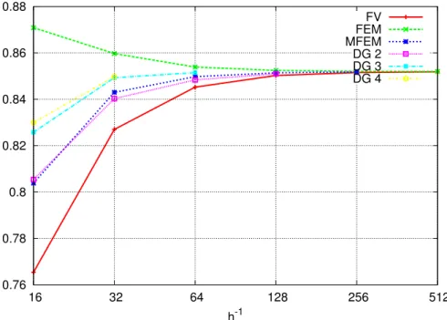
Figure 11: The overall flux F for the random permeability field 2D problem with correlation length of 1/16 calculated with diferent discretization schemes and successive grid refinement, rectangle grid discretization.

16 0.765417 0.803858 0.805419 0.825815 0.82999 0.870887 32 0.827035 0.843016 0.840281 0.849335 0.849788 0.859714 64 0.845258 0.849771 0.848381 0.851502 0.853922

128 0.85026 0.851424 0.851004 0.852462

256 0.851545 0.851836 0.852078

512 0.851872 0.851995

Table 9: The overall flux F for the random permeability 2D field with correlation length of 1/16, rectangles.

(18)

h^-1

FEM MFEM DG 2 DG 3 DG 4

0.75 0.8 0.85 0.9 0.95 1 1.05 1.1

16 32 64 128 256 512

Figure 12: The overall flux F for the random permeability field 2D problem with correlation length of 1/16 calculated with diferent discretization schemes and successive grid refinement, triangle grid discretization.

128 0.850556 0.846326 0.851841 256 0.851618 0.848221

512 0.849876

Table 10: The overall flux F for the random permeability 2D field with correlation length of 1/16, triangles.

8 0.832339 0.879213 0.882525 0.984478

16 0.910224 0.932414 0.958893

32 0.938126 0.951348

64 0.946078 0.949462

128 0.94814 0.948991

Table 11: The overall flux F for the random permeability 3D field with correlation length of 1/8, cuboids.