The Finite Volume Method

The Finite Volume Method

Heiner Igel

Department of Earth and Environmental Sciences

Ludwig-Maximilians-University Munich

1 Introduction Motivation History

Finite Volume in a Nutshell

2 Ingredients

The Finite-Volume Method via Conservation Laws The Lax-Wendroff Scheme

3 The Finite-Volume Method: Scalar Advection

4 The Finite-Volume Method for Elastic Waves Homogeneous Case

Heterogeneous Case

5 The Finite-Volume Method via Gauss’ Theorem

Introduction Motivation

Motivation

Robust

Simple concept Irregular grids Explicit method

Find solution for strongly

heterogeneous paramters and

discontinuities

First applications in plasma physics (Hermeline, 1993) and computational fluids (Versteeg and Malalasekera, 1995)

Discrete version of the divergence theorem was used for seismic wave propagation (Dormy and Tarantola, 1995)

Comparing and quantifying the accuracy of wave propagation of the finite volume method was done by Kaeser et al. 2001

Leveque, 2001 presented a natural consequence of conservation laws

Dumbser et al., 2007a presented the arbitrary high-order scheme

(ADER) to the finite-volume method

Introduction History

History

In its basic form it takes an entirely lo- cal viewpoint in the sense that the solution field q(x,t) is tracked inside a cell. The field is approximated by an average quantity Q _i ⁿ inside cell C as:

Q _i ⁿ = 1 dx

Z

C

q(x , t)dx

Introduction Finite Volume in a Nutshell

Finite Volume in a Nutshell

Tracking the change of the values with time inside each cell Q _i ⁿ⁺¹ − Q _i ⁿ

dt = F _i−1/2 ⁿ − F _i+1/2 ⁿ dx

Assuming the flux depends only on the adjacent Q _i ⁿ values (for left boundary)

F _i−1/2 ⁿ = f (Q ⁿ _i−1 , Q ⁿ _i )

The requirement of conservation for a transport problem leads to the advection equation of the form

∂ _t q(x , t) + a ∂ _x q(x , t) = 0

where a is the transport velocity

For the constant-coefficient advection problem the flux terms obviously are

F _i−1/2 ⁿ = aQ _i−1 ⁿ F _i+1/2 ⁿ = aQ _i ⁿ

where a is the advection velocity. With these definitions we obtain a fully discrete extrapolation scheme as

Q _i ⁿ⁺¹ = Q _i ⁿ + a dt

dx (Q _i−1 ⁿ − Q _i ⁿ )

A considerable better solution is the Lax-Wendroff scheme given as Q _i ⁿ⁺¹ = Q _i ⁿ − adt

2dx (Q _i+1 ⁿ − Q _i−1 ⁿ ) + 1 2 ( adt

dx ) ² (Q _i−1 ⁿ − 2Q _i ⁿ + Q _i+1 ⁿ )

which is second-order accurate and much less dispersive.

Ingredients

Ingredients

To describe what is happening we put ourselve into a finite volume cell

that we denote as C and denote the boundaries as x ∈ x ₁ , x ₂ . We

further assume a positive advection speed a.

Ingredients The Finite-Volume Method via Conservation Laws

The Finite-Volume Method via Conservation Laws

The total mass of any quantity inside the cell is Z x

x

q(x , t)dx

and a change in time can only be due to fluxes across the left and/or right cell boundaries. Thus

∂ _t Z x

x

q(x, t)dx = F ₁ (t ) − F ₂ (t)

where F _i (t) are rates (e.g., in g/s) at which the quantity flows through

the boundaries.

If we assume advection with a constant transport velocity a this flux is given as a function of the values of q(x , t) as

F → f (q(x , t)) = aq(x , t) in other words

∂ t

Z x

x

q(x, t)dx = f (q(x ₁ , t)) − f (q(x ₂ , t))

This is called the integral form of a hyperbolic conservation law.

Ingredients The Finite-Volume Method via Conservation Laws

The Finite-Volume Method via Conservation Laws

Using the definition of integration and antiderivates to obtain

∂ _t Z x

x

q(x , t)dx = − Z x

x

∂ _x f(q(x , t))dx Z x

x

[∂ _t q(x , t) + ∂ _x f (q(x , t))] dx = 0

which leads to the well-known partial-differential equation of linear advection

∂ t q(x, t) + ∂ x f(q(x , t)) = 0

Instead of working on the field q(x,t) itself we approximate the integral of q(x,t) over the cell C by

Q _i ⁿ ≈ 1 dx

Z

C

q(x , t ⁿ )dx

This is the average value of q(x , t) in-

side the cell.

Ingredients The Finite-Volume Method via Conservation Laws

Upwind scheme

In order to find an extrapolation scheme to approximate the future state of our finite-volume cells we integrate the integral form of a hyperbolic conservation law.

Z

C

q(x, t ⁿ⁺¹ )dx − Z

C

q(x , t ⁿ )dx

= Z t

t

f (q(x _L , t)dt − Z t

t

f (q(x _R , t)dt

where we used the definitions C → [x ₁ , x ₂ ] = [x _L , x _R ], rearranged terms, and divided by dx in order to recover the average cell values.

This equation is exact!

Using the following terms for the fluxes at the boundaries F _L,R ⁿ =

Z t

t

f (q(x _L,R , t))dt

we obtain a time-discrete scheme for the average values of our solution field q(x,t)

Q _i ⁿ⁺¹ = Q ⁿ _i − dt

dx (F _R ⁿ − F _L ⁿ )

where the upper index n denotes time level t n = n ∗ dt and the lower

index i denotes cell C i of size dx .

Ingredients The Finite-Volume Method via Conservation Laws

Upwind scheme

Figure : For the linear advection problem we can analytically predict where

the tracer will be located after time dt . The value of q(x

, t

) will be exactly

the same as q(x

− adt , t

). We can use this information to predict the new

cell average Q

.

We thus seek to approximate the next cell update Q ⁿ⁺¹ _i knowing that Q _i ⁿ⁺¹ ≈ q(x _i , t ⁿ⁺¹ ) = q(x _i − adt, t ⁿ )

The new cell average analytically by adding the appropriate mass flowing via the left boundary by interpolation

Q ⁿ⁺¹ _i = Q _i−1 ⁿ + dx − adt

dx (Q _i ⁿ − Q _i−1 ⁿ ) Q ⁿ⁺¹ _i = Q _i ⁿ (1 − adt

dx ) + Q _i−1 ⁿ adt dx .

After re-arranging we finally obtain a fully discrete scheme Q _i ⁿ⁺¹ = Q _i ⁿ − adt

dx (Q _i ⁿ − Q _i−1 ⁿ )

Ingredients The Finite-Volume Method via Conservation Laws

Upwind scheme

Stability criterion:

| adt dx | ≤ 1

Upwind scheme is of 1st order accuracy only and very dispersive.

Therefore it is not accurate enough to be of any use for actual

simulation tasks.

Ingredients The Lax-Wendroff Scheme

The Lax-Wendroff Scheme

Our goal is to find solutions to ∂ t Q + a∂ x Q = 0. We start by using the Taylor expansion to extrapolate Q(x , t ) in time to obtain

Q(x , t ⁿ⁺¹ ) = Q(x , t ⁿ ) + dt∂ t Q(x , t ⁿ ) + 1

2 dt ² ∂ _t ² Q(x , t ⁿ ) + . . . From the governing equation we can also state by additional differentiations

∂ _t ² Q = −a∂ _x ∂ t Q

∂ _x ∂ _t Q = ∂ _t ∂ _x Q = ∂ _x (−a∂ _x Q)

∂ _t ² Q = a ² ∂ _x ² Q

noting that we just derived the 2nd order form of the acoustic wave

equation.

Replacing time derivatives by the equivalent expressions containing space derivatives only and obtain

Q(x, t ⁿ⁺¹ ) = Q(x, t ⁿ ) − dta∂ x Q(x , t ⁿ ) + 1

2 dt ² a ² ∂ _x ² Q(x, t ⁿ ) + . . . Using central differencing schemes for both space derivatives

∂ _x Q(x, t ⁿ ) ≈ Q _i+1 ⁿ − Q ⁿ _i−1 2dx

∂ _x ² Q(x, t ⁿ ) ≈ Q _i+1 ⁿ − 2Q ⁿ _i + Q _i−1 ⁿ dx ²

we finally obtain a fully discrete second-order scheme Q _i ⁿ⁺¹ = Q _i ⁿ − adt

2dx (Q _i+1 ⁿ − Q _i−1 ⁿ ) + 1 2 ( adt

dx ) ² (Q _i+1 ⁿ − 2Q _i ⁿ + Q _i−1 ⁿ )

known as the Lax-Wendroff scheme.

Ingredients The Lax-Wendroff Scheme

The Lax-Wendroff Scheme

Using standard finite-difference considerations without making use of flux concepts.

By extending the finite-volume method towards higher order to approximate the solution inside the finite volume as a piecewise linear function.

The choice of slope considered then determines the specific 2nd order numerical scheme that evolves.

The Lax-Wendroff scheme can also be interpreted as a finite-volume method by considering the flux functions

F _L ⁿ = 1

2 a(Q ⁿ _i−1 + Q _i ⁿ ) − 1 2

dt

dx a ² (Q _i ⁿ − Q _i−1 ⁿ ) F _R ⁿ = 1

2 a(Q ⁿ _i + Q _i+1 ⁿ ) − 1 2

dt

dx a ² (Q _i+1 ⁿ − Q ⁿ _i )

The Finite-Volume Method:

Scalar Advection

The Finite-Volume Method: Scalar Advection

The Finite-Volume Method: Scalar Advection

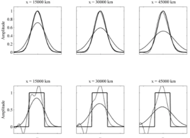
We proceed with implementing the two numerical schemes 1) the upwind method and 2) the Lax-Wendroff scheme. Recalling their formulations

Q _i ⁿ⁺¹ = Q _i ⁿ − adt

dx (Q _i ⁿ − Q _i−1 ⁿ ) and

Q _i ⁿ⁺¹ = Q _i ⁿ − adt

2dx (Q _i+1 ⁿ − Q _i−1 ⁿ ) + 1 2 ( adt

dx ) ² (Q _i+1 ⁿ − 2Q _i ⁿ + Q _i−1 ⁿ ) Using a spatial initial condition, a Gauss function

Q(x, t = 0) = e ^−1/σ

^{(x −x}

⁾

that is advected with speed c = 2500m/s. The analytical solution to this problem is a simple translation of the initial condition to

x = x ₀ + ct , where t = idt is the simulation time at time step i.

Parameter Value

x _max 75000 m

nx 6000

c 2500 m/s

dt 0.0025 s

dx 12.5 m

0.9

σ (Gauss) 200 m

x ₀ 1000 m

f o r i = 1 : n t ;

% upwind

i f method== ’ upwind ’, f o r j = 2 : nx−1,

% f o r w a r d ( upwind ) ( c > 0 ) dQ( j ) = (Q( j )−Q( j−1))/ dx ; end

% t i m e e x t r a p o l a t i o n Q=Q−d t∗c0∗dQ ; end

% Lax Wendroff

i f method == ’ Lax−Wendroff ’, f o r j = 2 : nx−1,

% f o r w a r d ( upwind ) ( c > 0 ) dQ1 ( j ) = (Q( j +1)−2∗Q( j ) +Q( j−1));

dQ2 ( j ) =Q( j +1)−Q( j−1);

end

% t i m e e x t r a p o l a t i o n

Q=Q−c /2∗d t / dx .∗dQ2+ . 5∗( c∗d t / dx ) . ^ 2 .∗dQ1 ; end

% Boundary c o n d i t i o n

% p e r i o d i c Q( 1 ) =Q( nx−1);

% a b s o r b i n g Q( nx ) =Q( nx−1);

end

The Finite-Volume Method: Scalar Advection

The Finite-Volume Method: Scalar Advection

Implemement periodic and absorbing boundary conditions with the statements

Periodic: Q ₁ ⁿ = Q _nx−1 ⁿ Absorbing: Q _nx ⁿ = Q _nx−1 ⁿ

Figure : Boundary conditions. Absorbing, or circular boundary conditions can be implemented by using ghost cells outside the physical domain

x ∈ [x

, x

].

Figure : Top: Snapshots of an advected Gauss function (analytical solution, thick

solid line) are compared with the numerical solution of the 1st order upwind method

(thin solid line) and the 2nd order Lax-Wendroff scheme (dotted line) for increasing

propagation distances. Bottom: The same for a box-car function.

The Finite-Volume Method for Elastic Waves

The Finite-Volume Method for

Elastic Waves

Source-free version of the coupled first-order elastic wave equation

∂ t v − 1

ρ ∂ x σ = 0

∂ _t σ − µ∂ _x v = 0 .

We proceed by writing this equation in matrix-vector notation

∂ t Q + A∂ _x Q = 0

where Q = (σ, v ) is the vector of unknowns and matrix A contains the parameters

A =

0 −1/ρ

−µ 0

The Finite-Volume Method for Elastic Waves

The Finite-Volume Method for Elastic Waves

The problem hereby is that these eqations are coupled. What needs to be done is to demonstrate the hyperbolicity of the wave equation in this form, i.e. show that A is diagonalizable.

In the case of a quadratic matrix A with shape m × m leads to an eigenvalue problem. If we were able to obtain eigenvalues λ p such that

Ax _p = λ p x _p , p = 1, ..., m we get a diagonal matrix of eigenvalues

Λ =





 λ ₁

. ..

λ m







and the corresponding matrix R containing the eigenvectors x p in each column

R = (x ₁ |x ₂ | . . . |x _p ) .

The Jacobian matrix A can now be expressed with the definitions A = RΛR ⁻¹

Λ = R ⁻¹ AR .

Applying these definitions to above equation we obtain R ⁻¹ ∂ t Q + R ⁻¹ RΛR ⁻¹ ∂ x Q = 0 and introducing the solution vector W = R ⁻¹ Q results in

∂ _t W + Λ∂ _x W = 0 .

The Finite-Volume Method for Elastic Waves

The Finite-Volume Method for Elastic Waves

What remains to be shown is that in our specific case A has real eigenvalues. These are easily determined as λ _1,2 = ± p

µ/ρ = ±c, corresponding to the shear velocity c. For the eigenvectors we obtain

r _1,2 = ±ρc

1

interestingly enough containing as first elements values of the seismic impedance Z = ρc that is relevant for the reflection behaviour of seismic waves. Thus, the matrix R and its inverse are

R =

Z −Z

1 1

, R ⁻¹ = 1 2Z

1 Z

−1 Z

.

The wave equation in the rotated eigensystem can be stated as

∂ _t w ₁

w ₂

+

−c 0

0 c

∂ _x w ₁

w ₂

= 0

with the simple general solution w _1,2 = w _1,2 ⁽⁰⁾ (x ± ct), where the upper index 0 stands for the initial condition.

The initial condition also fullfills W ⁽⁰⁾ = R ⁻¹ Q ⁽⁰⁾ . We can therefore relate the so-called characteristic variables w _1,2 to the initial conditions of the physical variables as

w ₁ (x , t) = 1

2Z (σ ⁽⁰⁾ (x + ct) + Zv ⁽⁰⁾ (x + ct )) w ₂ (x , t) = 1

2Z (−σ ⁽⁰⁾ (x − ct ) + Zv ⁽⁰⁾ (x − ct))

The Finite-Volume Method for Elastic Waves

The Finite-Volume Method for Elastic Waves

Obtaining the final analytical solution for velocity v and stress σ as σ(x , t) = 1

2 (σ ⁽⁰⁾ (x + ct ) + σ ⁽⁰⁾ (x − ct )) + Z

2 (v ⁽⁰⁾ (x + ct ) − v ⁽⁰⁾ (x − ct)) v (x , t) = 1

2Z (σ ⁽⁰⁾ (x + ct) − σ ⁽⁰⁾ (x − ct )) + 1

2 (v ⁽⁰⁾ (x + ct ) + v ⁽⁰⁾ (x − ct)) . In compact form this solution can be expressed as

Q(x , t) =

m

X

p=1

w _p (x, t)r _p

meaning that any solution is a sum over weighted eigenvectors, a

superposition of m waves.

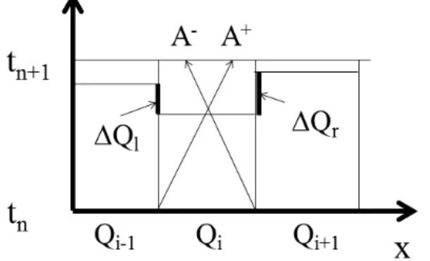
Riemann problem, homogeneous

case. Top: A discontinuity ∆Q is

located at x = 0 as initial condition to

the advection equation (e.g., as initial

stress discontinuity). Bottom: The

discontinuity propagates along

characteristic curves in the space-time

domain. The figure illustrates adjacent

cells and two time levels t

and t

.

Two waves propagate in opposite

direction modifying the values in the

cells adjacent to x = 0.

The Finite-Volume Method for Elastic Waves Homogeneous Case

Homogeneous Case

The solution to our problem is a superposition of weighted

eigenvectors r _p , in our case p = 1, 2. Therefore, we can decompose the discontinuity jump into these eigenvectors according to

∆Q = Q _r − Q _l = α 1 r ₁ + α 2 r ₂ Rα = ∆Q

α = R ⁻¹ ∆Q

where R is the matrix of eigenvectors as defined above and α are

unknown weights.

Decompose the solution into positive (right-propagating) and negative (left-propagating) eigenvalues

Λ ⁻ =

−c 0

0 0

, Λ ⁺ = 0 0

0 c

Then we can derive matrices A ^± - corresponding to the advection velocity in the scalar case

A ⁺ = RΛ ⁺ R ⁻¹

A ⁻ = RΛ ⁻ R ⁻¹

The Finite-Volume Method for Elastic Waves Homogeneous Case

Homogeneous Case

Figure : The constant average cell values of Q are illustrated for three adjacent cells

i − 1, i, i + 1. The eigenvector decomposition leads to wave A

propagating from the

left boundary with velocity c in to cell i and wave A

propgating with velocity −c into

cell i from the right boundary. This determines the flux of discontinuities ∆Q

into cell

i by the amount dt/dx ∆Q

.

We are ready to formulate an upwind finite-volume scheme for any multi-dimensional linear hyperbolic system:

∆Q _l = Q _i − Q _i−1

∆Q _r = Q _i+1 − Q _i Q ⁿ⁺¹ _i = Q ⁿ _i − dt

dx (A ⁺ ∆Q _l + A ⁻ ∆Q r ) . We can relate this formulation to the very basic flux concept

F _l = A ⁺ ∆Q _l

F _r = A ⁻ ∆Q _r .

The Finite-Volume Method for Elastic Waves Homogeneous Case

Homogeneous Case

The 1st order upwind solution is of no practical use because of its strong dispersive behaviour.

= ⇒The 2nd order Lax-Wendroff scheme

The high-order scheme does not necessitate the separation into eigenvectors and the Jacobian matrix A can be used in its original form. The extrapolation scheme reads

Q ⁿ⁺¹ _i =Q ⁿ _i − dt

2dx A(Q ⁿ _i+1 + Q ⁿ _i−1 ) + 1

2 dt dx

2

A ² (Q ⁿ _i−1 − 2Q ⁿ _i + Q ⁿ _i+1 ) .

Parameter Value

x max 10000 m

nx 800

c 2500 m/s

ρ 2500 kg/m ³

dt 0.025 s

dx 12.5 m

0.5

σ (Gauss) 200 m

x ₀ 5000 m

% S p e c i f i c a t i o n s Q=zeros( [ 2 , nx ] ) ; Qnew=zeros( [ 2 , nx ] ) ;

( . . . )

% I n i t i a l c o n d i t i o n

Qnew ( 1 , : ) =exp(−1./ s i g ^2∗( x−x0 ) . ^ 2 ) ;

% Time e x t r a p o l a t i o n f o r i = 1 : n t ;

% Lax−Wendroff Q=Qnew ;

f o r j = 2 : nx−1,

dQ1=Q ( : , j +1)−Q ( : , j−1);

dQ2=Q ( : , j−1)−2∗Q ( : , j ) +Q ( : , j + 1 ) ;

Qnew ( : , j ) = Q ( : , j )−d t / ( 2∗dx )∗A∗dQ1 . . . + 1 . / 2 .∗( d t / dx ) ^ 2 ∗A^2 ∗dQ2 ; end

% Absorbing b o u n d a r i e s Qnew ( : , 1 ) = Qnew ( : , 2 ) ; Qnew ( : , nx ) =Qnew ( : , nx−1);

end

% P l o t t i n g ( . . . ) end

The Finite-Volume Method for Elastic Waves Homogeneous Case

Result

The stress-velocity system is advected

for an initial condition of Gaussian

shape (top, dashed line, scaled by

factor 1/2). Top: Stress snapshot at

time t = 1.5s. Bottom: Velocity

snapshot at the same time. In both

cases analytical solutions are

superimposed.

Top: Single discontinuity separating two regions with different properties.

Bottom: Velocities and impedances

on both sides of the discontinuity. The

Riemann problem solves the problem

of how waves on both sides are

partitioned.

The Finite-Volume Method for Elastic Waves Heterogeneous Case

Heterogeneous Case

Mathematically the solution still has to consist of a weighted sum over eigenvectors that now describe solutions in the left and right parts.

∆Q = α ₁ −Z _l

1

+ α ₂ Z r

1

for some unknown scalar values α _1,2 . This can be written as a linear system of the form

R _lr α = ∆Q

where α is a vector and the matrices with the eigenvector are R _lr =

−Z _l Z r

1 1

, R ⁻¹ _lr = 1 Z _l + Z _r

−Z _l Z r

1 1

Using the R matrix for cell boundaries separating cells with different (constant) properties. Again we separate into left- and

right-propagating eigenvalues within cell i Λ ⁻ =

−c _i 0

0 0

, Λ ⁺ =

0 0 0 c _i

and using the definitions R _l =

−Z _i−1 Z _i

1 1

, R _r =

−Z _i Z _i + 1

1 1

for the eigenvectors describing the solutions around the left and right boundaries we can determine the corresponding advection terms as

A ⁺ = R _l Λ ⁺ _l R ⁻¹ _l

A ⁻ = R _r Λ ⁺ _r R ⁻¹ _r

The Finite-Volume Method for Elastic Waves Heterogeneous Case

Heterogeneous Case

Leading to the 1st order upwind extrapolation scheme for the solution vector Q _i in the general heterogeneous case

∆Q _l = Q _i − Q i−1

∆Q _r = Q _i+1 − Q _i Q ⁿ⁺¹ _i = Q ⁿ _i − dt

dx (A ⁺ ∆Q _l + A ⁻ ∆Q _r )

= ⇒ too dispersive but interesting side effect!

Let us take the eigenvector (i.e., wave) propagating in the left domain.

What does this imply for the wave propagating in the right domain?

∆Q = Z _l

1

We need to determine how the waves are partitioned given the

discontinuous material parameters described by matrix R _lr . This leads to the coefficients α as

α = R ⁻¹ _lr ∆Q

= 1

Z _l + Z _r

−1 Z r

1 Z _l Z _l

1

=









Z

−Z

Z

+Z

2Z

Z

+Z









=







 R T









that are the well known transmission and reflection coefficients for

vertical incidence at a material discontinuity.

The Finite-Volume Method for Elastic Waves Heterogeneous Case

Heterogeneous Case

Reflection and transmission coefficients. Seismic waves incident perpendicular to a material

discontinuity are reflected and

transmitted according to coefficients R and T . These coefficients can be derived via the Riemann problem used to develop flux schemes for

finite-volume methods.

Finally, we present the 2nd order scheme for the general heterogeneous results and a simulation example.

A _i−1/2 = 1

Z _i−1 + Z _i

c _i Z _i − c i−1 Z i−1 (c i−1 + c _i )Z i−1 Z _i c _i−1 + c _i c _i Z _i−1 − c _i−1 Z _i

A _i+1/2 = 1

Z _i + Z _i+1

c _i+1 Z _i+1 − c _i Z _i (c _i + c _i+1 )Z _i Z _i+1 c _i + c _i+1 c _i+1 Z _i − c _i Z _i+1

. With these definitions we can formulate the Lax-Wendroff extrapolation scheme for elastic waves in heterogeneous material

Q ⁿ⁺¹ _i =Q ⁿ _i − dt 2dx

A _i−1/2 (Q ⁿ _i − Q ⁿ _i−1 ) + A _i+1/2 (Q ⁿ _i+1 − Q ⁿ _i ) + 1

2 ( dt dx ) ²

h

A ² _i+1/2 (Q ⁿ _i+1 − Q ⁿ _i ) − A ² _i−1/2 (Q ⁿ _i − Q ⁿ _i−1 )

i

The Finite-Volume Method for Elastic Waves Heterogeneous Case

Example

Parameter Value

x max 10000 m

nx 800

c _l 2500 m/s

c r 5000 m/s

ρ 2500 kg/m ³

dt 0.025 s

dx 12.5 m

0.5

σ (Gauss) 200 m

x ₀ 5000 m

% I n i t i a l i z a t i o n o f f l u x m a t r i c e s f o r i = 2 : nx−1,

Am ( : , : , i ) = 1 / ( Z ( i−1)+Z ( i ) ) ∗ . . .

[ c ( i )∗Z ( i )−c ( i−1)∗Z ( i−1) ( c ( i−1)+c ( i ) )∗Z ( i−1)∗Z ( i ) ; . . . c ( i−1)+c ( i ) ´

c ( i )∗Z ( i−1)−c ( i−1)∗Z ( i ) ] ; Ap ( : , : , i ) = 1 / ( Z ( i ) +Z ( i + 1 ) ) ∗ . . .

[ c ( i +1)∗Z ( i +1)−c ( i )∗Z ( i ) ( c ( i ) + c ( i + 1) )∗Z ( i )∗Z ( i + 1 ) ; . . . c ( i ) + c ( i +1)

c ( i +1)∗Z ( i )−c ( i )∗Z ( i +1) ] ; end

% Time e x t r a p o l a t i o n f o r i = 1 : nt , ( . . . )

f o r j = 2 : nx−1, dQl=Q ( : , j )−Q ( : , j−1);

dQr=Q ( : , j +1)−Q ( : , j ) ; Qnew ( : , j ) = Q ( : , j ) . . .

−d t / ( 2∗dx )∗(Am ( : , : , j )∗dQl+Ap ( : , : , j )∗dQr ) . . . + 1 . / 2 .∗( d t / dx ) ^ 2∗( Ap ( : , : , j )^2∗dQr . . .

−Am ( : , : , j )^2∗dQl ) ; end

( . . . )

% Absorbing b o u n d a r i e s Qnew ( : , 1 ) = Qnew ( : , 2 ) ; Qnew ( : , nx ) =Qnew ( : , nx−1);

( . . . ) end

The Finite-Volume Method via Gauss’ Theorem

The Finite-Volume Method via

Gauss’ Theorem

Gauss’ theorem states that the outward flux of a vector field Q _i (x , t) through a closed surface S is equal to the volume integral of the divergence over the volume V inside the surface at some time t.

Mathematically this can be expressed as Z

V

∂ _i Q _i dV = Z

S

n _i Q _i dS

where n _i are the components of the local surface normal vector.

Note:

Not restricted to vector fields −→ any tensor field Q _i,j...

Applies also to scalar fields Q(x,t)

The Finite-Volume Method via Gauss’ Theorem

The Finite-Volume Method via Gauss’ Theorem

Assuming the gradient of the solution field is smooth enough and can be assumed constant inside volume V we can take it out of the integral and obtain an expression for the derivative as a function of an integral over a surface S with segements dS in 3D or a line with segments dL surrounding a surface S in 2D

∂ _i Q Z

V

dV = Z

S

n _i QdS

∂ _i Q _3D = 1 V

Z

S

n _i QdS

∂ i Q _2D = 1 S

Z

L

n _i QdL

Concept of numerical gradient calcu- lation using Gauss’ theorem illustrated in 2D. The constant gradient of a scalar field Q inside the finite vol- ume S is approximated as ∂ _i Q = 1/S P

α n _i ^α dL ^α Q ^α . The polygon can

have any shape.

The Finite-Volume Method via Gauss’ Theorem

The Finite-Volume Method via Gauss’ Theorem

Once a discretization of surfaces or surrounding lines is found we can de- velop a discrete scheme replacing the integrals in the above equations by sums to obtain

∂ _i Q _3D ≈ 1 S

X

α

n _i ^α dS ^α Q ^α

∂ i Q _2D ≈ 1 L

X

α

n ^α _i dL ^α Q ^α .

The importance here is that this de-

scription is entirely independent of the

shape of a particular volume.

A rhombus-shaped finite volume cell is described by four edge points.

P ₁ = (−∆ ₁ , 0), P ₂ = (+∆ ₁ , 0), P ₃ = (0, −∆ ₂ ), P ₄ = (0, +∆ ₂ ) with the length of the sides given by ` =

q

∆ ² ₁ + ∆ ² ₂ and the surface S = 2∆ ₁ ∆ ₂ . The four normal vectors are defined by

n _2,4 = ∆ ₂

∆ ₁

; n _4,1 = −∆ ₂

∆ ₁

; n _1,3 =

−∆ ₂

−∆ ₁

; n _3,2 = ∆ 2

−∆ ₁

.

The Finite-Volume Method via Gauss’ Theorem

The Finite-Volume Method via Gauss’ Theorem

We now have all components to apply previous equation in the 2D case. We integrate along the paths suggested in the figure to obtain

∂ ₁ Q = 1 S ( `

2 Q ₁ (− ∆ ₂

` − ∆ ₂

` ) + `

2 Q ₂ ( ∆ ₂

` + ∆ ₂

` ) + `

2 Q ₃ (− ∆ ₂

` + ∆ ₂

` ) + `

2 Q ₄ ( ∆ ₂

` − ∆ ₂

` ))

= 1

S (−Q ₁ ∆ ₂ + Q ₂ ∆ ₂ )

= Q ₂ − Q ₁ 2∆ ₁

for the 1st derivative of Q w.r.t. x.

Example of elastic wave simulations in

2D using difference operators based

on the finite-volume approach (Kaeser

2001b). In this example an unstruc-

tured grid follows a free-surface topog-

raphy with ghost cells outside the sur-

face to implement stress-free boundary

conditions.

The Finite-Volume Method via Gauss’ Theorem

Summary

The finite-volume method naturally follows from discretizing conservation equations considering fluxes between finite-volume cells of averaged solution fields.

The fluxes across boundaries during an extrapolation step are estimated using solutions to the Riemann problem.

The Riemann problem considers the advection of a single jump discontinuity taking into account the analytical solution of the homogeneous problem. It allows an analytical prediction of how much of the material (energy, stress, etc.) to be conserved enters into or leaves a cell.

The lowest order finite-volume solution to the advection equation leads to a

finite-difference algorithm with a forward (or backward) spatial differencing

scheme, depending on the advection direction. This is called an upwind scheme.

First-order finite-volume schemes are highly dispersive and not appropriate for the solution of wave propagation problems. The 2nd order Lax-Wendroff scheme does a much better job.

The problem of elastic wave propagation can be formally cast as a 1st order hyperbolic problem. Therefore - only with slight modifications - the fundamental schemes developed for the scalar advection problem can be applied to elastic wave propagation.

In the finite-volume method the problem of estimating partial derivatives (finite differences) is replaced by the requirement to accurately calculate fluxes across cell boundaries.

A main advantage of the finite-volume method is the fact that the scheme can be easily applied to volume cells of any shape.

Finite-volume schemes for arbitrary high-order reconstructions inside the cells

and high-order time-extrapolation schemes have been developed but not used

extensively in seismology.

The Finite-Volume Method via Gauss’ Theorem

Comprehension questions

1 What is the connection between finite-volume methods and conservation equations?

2 What is meant by finite volumes, is there any difference to a finite element?

3 If you look at the uwpind approach to the scalar advection problem (Eq. ??), why is the finite-volume method so closely linked to staggered-grid finite-difference schemes? Explain.

4 What are the main advantages of finite-volume methods compared with finite-difference methods?

5 Explain in a qualitative way what the Riemann problem is and why it is so essential for finite-volume schemes.

6 In what areas of natural sciences are finite-volume schemes mostly used.

Explore the literature and try to give reasons.

7 What is numerical diffusion? Why is it relevant for finite-volume methods?

8 What is the connection between reflection/transmission coefficients of seismic waves and the finite-volume method?

9 The finite-volume method extrapolates cell averages. What strategies do you

see to extend the method to high-order accuracy?

10 Show that equation is a finite-difference solution to the equation ∂

Q − a∂

Q = 0 using a forward difference in space.

11 The stability criterion for the finite-volume method is cdt/dx ≤ 1. Starting with Fig. derive this stability criterion from first principles.

12 Starting with the advection equation ∂

Q − a∂

Q = 0 derive the second-order wave equation by applying the so-called Cauchy-Kovalevskaya procedure.

13 Following the finite-volume approach based on the divergence theorem calculate

the spatial derivative operator for the hexagonal cell.

The Finite-Volume Method via Gauss’ Theorem

Theoretical problems

14 The linear system for elastic wave propagation in 1D (transverse motion) is given in equation. The wave equation can also be formulated for compressional waves using the compressibility K as elastic constant. Reformulate the linear system for acoustic wave propagation and calculate the eigenvalues of the resulting Jacobian matrix A.

15 For either elastic or acoustic linear system derive the eigenvectors of Jacobian matrix A, the matrix of eigenvectors and its inverse.

16 Show that the superposition of left- and right-propagating stress and velocity waves are solutions to the linear system of equations for elastic wave propagation.

17 Show that a discontinuity of the form ∆Q = [1, 0] leads to an equi-partitioning of two seismic waves propagating in opposite directions. Start with the Riemann problem formulated for the homogeneous case.

18 Derive reflection and transmission coefficients for seismic waves with vertical

incidence by considering the Riemann problem for material discontinuity.

19 Determine the stability limit of the Lax-Wendroff scheme for the scalar advection equation. Is it the same as for the upwind scheme?

20 Create a highly unstructured 1D mesh and investigate the accuracy of the finite-volume method (Lax-Wendroff) for the scalar advection problem.

21 Investigate the concept of trapped elastic waves by injecting an initial condition in a low-velocity region. Use the Lax-Wendroff algorithm in 1D.

22 Implement circular boundary conditions in the 1D elastic Lax Wendroff solution.

Initiate a sinusoidal function f (x) = sin(kx ) that is advected in one direction.

Investigate the accuracy of the finite-volume scheme as a function of wavelength and propagation distance by comparing with the analytical solution.

23 The finite-volume method is supposed to conserve energy in the homogeneous case. Use the computer programs for scalar advection, set up an example and calculate the total energy in the system for each time step. Check whether it is conserved. Explore this problem for the heterogeneous case.

24 Scalar advection problem: Advect a Gaussian shaped waveform as long as you

can and extract the travel time difference with the analytical solution in an

automated way using cross-correlation. Plot the time error as a function or

propagation distance and your simulation parameters.