Open data travel demand synthesis for agent-based transport simulation: A case study of Paris and Île-de-France
Sebastian Hörla,b,∗, Milos Balaca
aInstitute for Transport Planning and Systems, ETH Zurich
bInstitut de Recherche Technologique SystemX, Palaiseau 91120, France
Abstract
Synthetic populations of travellers and their detailed mobility behaviour are an important basis for agent-based transport simulations, which are increasingly used in transport planning and research today.
While previous applications of such simulations put focus on analyzing policies and novel modes of transport, less importance is put on the aspects of data collection, processing and validation to create the disaggregate travel demand. This paper proposes an open-source and extendable pipeline for travel demand synthesis for Île-de-France, which establishes a clear path from raw data to the final demand consisting of households, persons, and trips with their respective attributes. The travel demand synthesis is based on open and publicly accessible data and can be easily transferable to other regions in France. By basing the process on open software and open data, the paper establishes a baseline not only for generating a fully replicable travel demand, but also enables researchers to perform replicable transport simulations.
While the proposed pipeline, which is runnable by any reader, is based on rather straightforward and data-driven algorithms, pathways are provided for extending the process. Additionally, methods for quality assessment of synthetic populations and travel demand are proposed and discussed.
Keywords: open, agent-based, transport, simulation, synthetic, population, Paris, Île-de-France
1. Introduction
Agent-based models have become popular in recent decades in many fields of science, mostly because they can model complex systems and interactions within. Importantly, they also allow the modeling of emergent behavior (Bonabeau, 2002). In transportation, traditionally, aggregated four-step models are used to evaluate new policies or infrastructure investments. However, these models fail to capture the
5
interactions between individuals and model transportation on an aggregated scale. They overlook the importance of individuals, their interaction, decisions, and behavior.
Furthermore, they are not readily adaptable to deal with new mobility solutions like car-sharing, bike- sharing, micro-mobility, inter-modality, or future mobility solutions and their operational challenges. It is then no wonder that agent-based models have also found an application in transportation science.
10
Unfortunately, unlike four-step models, agent-based models are challenging to build and maintain, and are usually very data-hungry.
The foundation of every agent-based model in transportation is a synthetic travel demand including a synthetic population of households and persons with sociodemographic attributes and their daily activity patterns in time and space. While there are efforts to document the process of obtaining the synthetic
15
travel demand, those are rarely reproducible, easily verifiable, or open-source. Therefore, they lack one or more of the following: the possibility to be validated by others; the possibility to be extended by others;
ease of adding new data or features; and access to the methods used and their documentation.
This paper builds upon the thinking that scientific work should be easily accessible, open-source, and reproducible. Therefore, we propose a fully automated and customizable open-source pipeline for travel
20
demand synthesis. The pipeline takes the raw data and, through various steps, produces a synthetic population. In this way, it allows us to reliably reproduce the required input data for many agent-based transport simulation frameworks. It reduces the effort of building and maintaining the synthetic travel demand.
∗Corresponding author
Email addresses: sebastian.horl@irt-systemx.fr(Sebastian Hörl),milos.balac@ivt.baug.ethz.ch(Milos Balac)
Furthermore, for the first time, with this approach, it is possible to perform sensitivity analysis, not
25
only on a static input population, but on the whole process of setting up a transport model from data processing to final simulation. The pipeline itself establishes a travel demand synthesis process based on straightforward data-driven algorithms. This way, it is a comprehensive benchmark for more advanced and novel algorithms, be it in travel demand synthesis (Bayesian networks, Markov models, and others), mode choice models, location assignment, or other components.
30
2. Background
A long-established approach to forecast transportation demand is to use four-step models. These aggregated models are a traditional way of evaluating policies for large infrastructure investments, and focus on large car and transit flows. Activity-based models emerged to overcome the aggregation drawback of these models. See Recker (1995); Axhausen and Gärling (1992); Kitamura (1988) for early reviews
35
of activity-based models and Rasouli and Timmermans (2014) for a more recent overview. They use various methods to schedule activities for individuals and make mode or destination choices, within a single framework. These models were the answer to the aggregation drawback of four-step models and the inability to model tour constraints.
Moreover, activity-based models were able to provide policy implications on many more dimensions
40
than four-step models. However, these models usually involve a range of econometric sub-models that need to be estimated, and later calibrated to fit the data. Unfortunately, many activity-based models only focus on a small number of regions, are not easily extendable, not open-source, or lack documentation to achieve reproducibility of studies. Examples of activity-based models are CEMDAP (Bhat et al., 2008), which is based on the Dallas-Fort Worth region in the USA, or the rule-based model TASHA (Hao,
45
2009), which is specifically designed for the Greater Toronto area in Canada. Another notable example of activity-based models is ActivitySim (ActivitySim, 2020). It is being developed as an open-source platform for activity-based travel modeling by multiple transportation agencies in the USA. Another framework that was developed through the same collaboration is PopulationSim. It creates a synthetic population that contains only the socio-demogrpahic attributes and household structures, but no travel demand,
50
based on the marginal data available from the USA census, which creates the basis for ActivitySim.
Agent-based models appeared as the need to model interactions between individuals became impor- tant. Today, this need becomes evident as many different transportation services co-exist, and they are used both in a competing and in a complementary fashion. Often, these forms of transport are highly dynamic as vehicles are managed on a minute-by-minute or second-by-second basis and therefore require
55
modeling on a shorter time-scale than activity-based models usually provide. Some examples of agent- based transport models are POLARIS (Auld et al., 2016), SimMobility (Adnan et al., 2016), SUMO (Lopez et al., 2018), or MATSim (Horni et al., 2016).
Some attempts to pair activity-based models with agent-based models exist. The advantage of activity- based models in this configuration is that the former are well-established and based on sophisticated
60
econometric models, often fed with years of available data sets. The latter can provide fine-grained spatial dynamics and emergent congestion patterns, originating from the detailed simulation of agent interactions. Combinations of activity- and agent-based models have, for instance, been performed for MATSim: Ziemke et al. (2015) apply CEMDAP to generate daily activity patterns for a model of the Berlin area, and Hao (2009) and Diogu (2019) pair MATSim with TASHA’s Toronto model. POLARIS
65
makes use of the activity-based model ADAPTS (Auld and Mohammadian, 2009).
Agent-based models are dependent on a synthetic travel demand as input data. The aim is then to simulate how agents behave on the transportation network and how they compete for the infrastructure.
Viegas and Martínez (2010), for instance, create a synthetic travel demand using a mobility survey.
They use statistical approaches and create an agent population for the region of Lisbon, Portugal, which
70
they later use in different agent-based studies (Martinez et al., 2015; Martinez and Viegas, 2017). In the ecosystem of MATSim, various synthetic populations exist, such as the models for Singapore (Erath et al., 2012) or Switzerland (Bösch et al., 2016; Hörl et al., 2019). While the approaches outlined below in this paper draw from the latter reference, here we propose a reproducible, open-source, and open data approach, contrary to the models of Singapore and Switzerland, which have restricted shareability due
75
to the proprietary nature of the underlying data sets. However, open data models exist for MATSim, such as the Open Berlin model (Ziemke et al., 2019b), Ruhr region in Germany (Ziemke et al., 2019a), or the older model of Santiago de Chile (Kickhofer et al., 2016), which can be named as the oldest open
data model in the MATSim ecosystem1. Based on publicly available data, Kamel et al. (2018) propose a first MATSim model including an open-source synthesis tool of the Île-de-France region in France,
80
which subsequently was transferred to case studies on the city of Rouen (Vosooghi et al., 2019a,b). Thus, open-data-based models exist, yet they are only documented as part of a more applied, larger-scope case study, whereas the details of the synthesis process are only described briefly in most cases. This arguably limits the reproducibility of not only those models, but also of the studies conducted with them.
Reproducibility has recently become an important topic in research in many fields. Articles emphasize
85
the lack of information or data for other researchers to be able to replicate studies published in scientific journals (Goodman et al., 2016; Chen et al., 2019; Stark, 2018; Boulton, 2016; Baker, 2016). While the necessary steps to ensure replicability of scientific findings can vary across the scientific disciplines, the researchers generally agree that in order to ensure reproducibility of research outcomes, the authors of a scientific study need to:
90
• provide access to the raw data used in the study or to provide enough details about their data collection methods
• provide access to the code/tools with which the data was processed before it was used in the study
• provide access to the software used in the study
• ensure that the set-up of the study is either explained in enough detail or it is provided as open-
95
source (in case the study requires implementation of a computer program), in order to ensure accessibility
National science foundations are also emphasizing the need for reproducibility in research. The U.S.
National Science Foundation states (Cacioppo et al., 2015): "reproducibility refers to the ability of a researcher to duplicate the results of a prior study using the same materials as were used by the original
100
investigator. That is, a second researcher might use the same raw data to build the same analysis files and implement the same statistical analysis in an attempt to yield the same result [...] Reproducibility is a minimum necessary condition for a finding to be believable and informative". The Swiss National Science Foundation (SNSF) requires, to ensure transparency and reproducibility of research findings, that all data used in the publications funded by SNSF is made publicly available, as long as it meets ethical
105
standards.
Based on this, we want to ensure reproducibility of the travel demand generated in this study by (1) publishing the software developed as open-source, (2) using only publicly available data, (3) documenting the processing methods in detail, and (4) ensuring that the complete process is accessible. While first three points are easily achievable, accessibility is not. In order to ensure accessibility for the wide range of
110
users, to regenerate or replicate the demand presented in this paper, we provide easy to follow instructions through the published documentation of the approach. To replicate the study presented here requires no previous programming skills or access to any commercial software. Even though the pipeline does not work as a GUI executable the effort needed to prepare it to run is minimal. Therefore, almost any researcher with access to internet can perform the presented study and obtain the same results. While
115
accessibility has been defined in a wider sense (e.g. Lovelace, 2020) including all potential users from the public, we believe that our framework is a valuable development toward that goal.
Furthermore, the paper at hand adds to the discussion in a number of ways. We provide:
• an integrated, open-source software pipeline to generate the synthetic travel demand from raw data, which can be extended and adapted by interested researchers or practitioners;
120
• synthetic travel demand, readily prepared for agent-based transport simulation, for the case of the Île-de-France region around Paris;
• thorough documentation of the synthesis process with basic data-driven approaches without the need for much calibration;
• the basis to ensure reproducibility of scientific agent-based studies in the Île-de-France region.
125
By that, we intend to foster open and reproducible research with agent-based models.
1Further models can be found at https://www.matsim.org/open-scenario-data
In addition, we invite researchers to test their specific methods for population synthesis, location assignment, and other aspects inside of an integrated pipeline. All code is available online (Appendix B), and the process is based on publicly available data. Methodologically, we intend to give ideas and first approaches for validating and verifying the quality of agent-based transport simulations, by examining
130
error properties of the whole synthesis process.
The remainder of the paper is structured as follows. Section 3 describes the synthesis process. In particular, the data sets used will be covered in detail, as well as the methods used. Section 4 analyzes the generated population for Île-de-France in terms of fit to reference data. Afterward, Section 5 provides a more detailed analysis of the influence of sampling rate and confidence in the results. We finish with a
135
discussion of the presented analyses in Section 6 and provide a final summary in Section 7. At this point, we would already like to point the reader to the glossary in Appendix A, which covers the abbreviations of data sets, concepts, and methods introduced throughout the paper.
3. Travel demand synthesis
Our synthesis pipeline aims to start with raw data sets, to transform them, to apply further models,
140
and arrive at a final synthetic travel demand on a person level that can be readily used in a downstream agent-based transport simulation. We intentionally apply rather simple, data-driven algorithms to es- tablish a baseline into which more sophisticated models can be integrated later on, with the ability to compare them against an established benchmark.
The proposed pipeline for Île-de-France consists of several steps that each draw from a specific data
145
set and apply a particular algorithm to make use of the data in the synthetic travel demand. Figure 1 shows the general setup of this pipeline. In a sequence of steps, a data set is created that contains a representation of all households in the region, with individual persons attached to them. Those persons have a sequence of trips and activities, which they perform during an average workday in Île-de-France.
While the household and person data sets contain rich sociodemographic information and their respective
150
home locations, the activity data set contains the purposes, times, durations, and locations of those activities. The trips data set additionally adds the duration of trips and the chosen mode of transport.
For this synthesis process, data sets are required, which are also summarized in Figure 1. Except for the regional household travel survey, all data sets are publicly available and can be obtained by any researcher from the respective websites. As we also provide the pipeline code, as open-source software, it
155
is, therefore, possible for anybody to recover the synthetic travel demand from raw data. While the quality can be improved, using the more fine-grained regional household travel survey, which is only available on request from the respective authorities, the national data set poses a viable open replacement.
Technically, the code is provided in two parts. The first part issynpp2, a generic Python package for chaining algorithms and code pieces (stages) in a larger pipeline setup. While it can be used in a general
160
way, it aims at providing a solid basis for travel demand synthesis and transport simulation applications.
The second part is the specific implementation of the Île-de-France use case, including the code for all data transformation, processing, and writing steps. The code is provided open source3. The Île-de-France pipeline is designed in a way that any researcher can download the necessary data sets and regenerate the synthetic travel demand for Île-de-France as it is described in this paper. Appendix B gives a first
165
overview and directions on how to set up and run the pipeline.
In the following, Section 3.1 gives an overview of the data sources used, while Section 3.2 describes the methods which are applied to them.
3.1. Data sources and cleaning
In the following sections, data sets shall be presented, which make it possible to create a full synthetic
170
travel demand for the Île-de-France region in France. The proposed process of synthesizing a travel demand, as outlined further below, is solely based on these data sets.
3.1.1. Spatial zoning system
In France, different spatial zoning systems are in use for statistical purposes. In this research, only a couple of them is used, mainly the ones that have the highest availability among the published data
175
sets. The reference data set is a shapefile containing the contours of all IRIS zones in France. Those
2https://github.com/eqasim-org/synpp
3https://github.com/eqasim-org/ile-de-france
Sociodemographics & Homes RP: Population census
Activity chains / Mobility patterns
Primary (work / education) destinations
Secondary (shopping / leisure / ... ) destinations
Sampling
Statistical matching
Origin/destination sampling
Assignment algorithm
Households
Persons Trips
Activities Household income
Spatial imputation ENTD: National household travel survey
EGT: Regional household travel survey
Filosofi: National tax registry
RP: Census with commute data SIRENE: Enterprise census
BPE: Facility data IRIS: Spatial zoning data BD-TOPO: Address database
Figure 1: General setup of the synthesis pipeline with the used data sets. All data sets are open and publicly available (green), except the regional household travel survey (yellow).
IRIS zones were introduced in 1999 and updated in 2008 to perform country-wide statistical analyses based on the national census. Each IRIS zone has an identifier that is divided into three parts: The first two digits denote thedépartement, which is an upper-level administrational unit, the following three digits identify a commune (municipality) within thisdépartement, and the last four digits describe the
180
statistical IRIS zone in that municipality. It is important to note that not allcommunes may be divided into IRIS, mainly if they have less than 10,000 inhabitants.
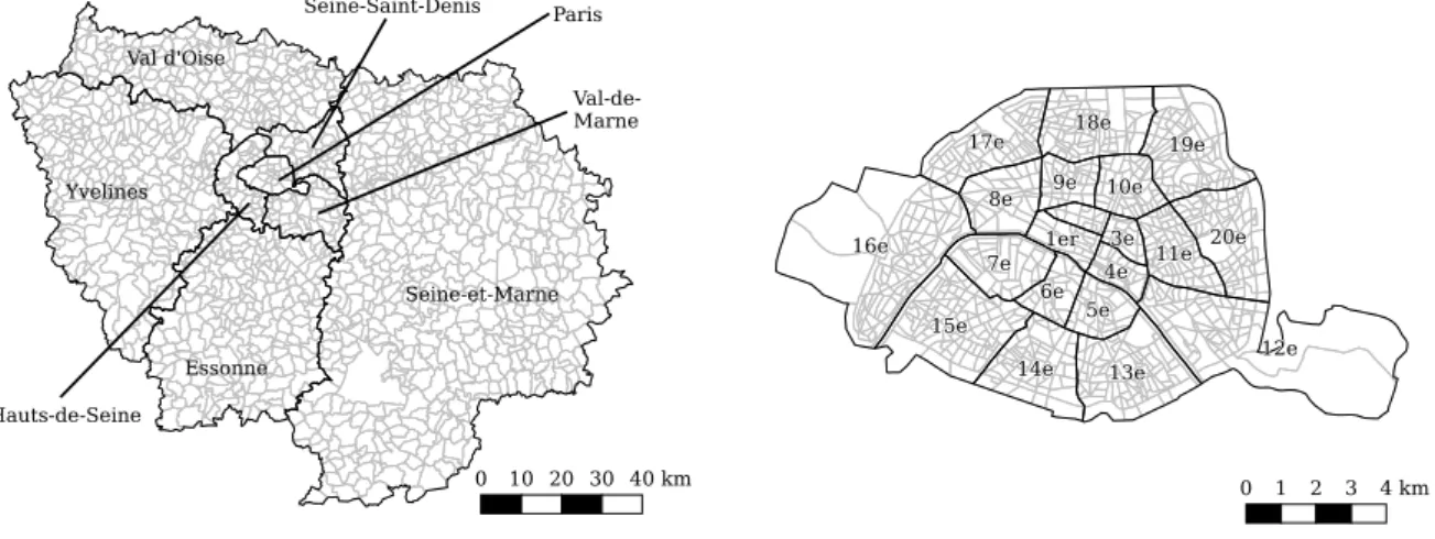
For the present study, only zones within the Île-de-Franceregion in France are considered. Those are all which lie in the departments of Paris (75), Seine-et-Marne (77), Yvelines (78), Essonne (91), Hauts- de-Seine (92), Seine-Saint-Denis (93), Val-de-Marne (94), and Val-d’Oise (95). Figure 2a shows the area
185
of the départements of Île-de-France and the communes into which they are divided. The city area of Paris is not divided into communes, but into 20 arrondissements. Their spatial extents are similar to those of the municipalities. Therefore, both communes and arrondissements are treated equally in the scope of our method. The segmentation of the Paris department intoarrondissements is shown in Figure 2b. In this case, also the further division into statistical IRIS zones is shown.
190
For the Île-de-France region, we work with eight departments, 1,296 municipalities, and 5,259 IRIS covering an area of around 12,000 km2.
3.1.2. National census
National census data for France (Recensement de la population, RP) is published byINSEE (National Institute of Statistics and Economic Studies) on an annual basis three years after that data has been
195
obtained. The latest available data set has been published in June 2018 and contains statistical informa- tion of a representative sample of the French population for the year 2015. For each household and each
Seine-et-Marne
Essonne Yvelines
Val d'Oise
Hauts-de-Seine
Seine-Saint-Denis Paris
Val-de- Marne
(a) Thedépartementsof the study area and thecommunesinto which they are divided.
(b) Thecommunes(arrondissements) of the study area and the IRISinto which they are divided. Note that also the surrounding municipalities are covered by similarly sized IRIS.
Figure 2: Spatial zoning of the study area
Structural attributes Person attributes Household attributes Spatial attributes
Household ID Age Household size IRIS ID*
Person ID Sex Number of cars Municipality ID*
Household weight Employed (yes/no) Department ID
Ongoing education (yes/no) Socio-professional category
Table 1: Attributes per person resulting from cleaning and analysis of the French census dataset. *Spatial attributes are only given if available.
person, numerous sociodemographic attributes are given, such as age, gender, household income, number of cars, and others. A statistical weight is assigned to each household, which makes the data compatible with previous publications of the data set and other surveys performed in France.
200
For most households, the identifier of their home IRIS is given, which allows for the protection of person-specific data, but makes it also possible to use the data for synthesis purposes, as in this study. If an IRIS has less than 200 inhabitants, only the identifier of the municipality is given (0.07% of weighted households). Also, some municipalities are not covered by IRIS at all, because the municipality itself has a low number of inhabitants. In those cases, only the identifier of the department is known (10.06% of
205
weighted households).
Nevertheless, the national census allows us to synthesize a population with spatially detailed sociode- mographic attributes. It is also fortunate that the census is given on the household-level, with specific persons being directly attached to those households. This structure makes it possible also to synthesize realistic household-level distributions of sociodemographic attributes.
210
The census data set for 2015 features a large sample of individually weighted person observations for France and its overseas territories. For the Île-de-France region, it lists around 4.3 million residents in 1.9 million households, which makes around 35% of the real population.
For its use in our approach, the individual dataset is further cleaned. The resulting attributes can be seen in Table 1. Households containing persons who have their principal place of employment or
215
education outside of Île-de-France are filtered out to restrict the study area to the region itself. These are 1.97% of the households containing 2.53% of all persons.
One attribute that requires further explanation is thesocio-professional category. It is a well-defined (INSEE, 2003) concept which classifies persons into eight categories: (1) agricultural workers, (2) artisans, merchants, self-employed, (3) leading positions and intellectual workers, (4) intermediate professions, (5)
220
employees, (6) workers, (7) retired, (8) others without employment.
In addition to the detailed data sets, INSEE also prepares aggregate datasets. These tables contain, for instance, an aggregated age distribution for each IRIS in France, including those whose inhabitants cannot be geolocalised in the individual data set. We use this dataset to enrich the zoning data with
information on the total number of inhabitants in each zone. Furthermore, we use the data as a reference
225
when comparing the characteristics of our synthetic population.
3.1.3. Origin-Destination commute flows
Along with the census data, information about the commuting behavior of the French population is published by INSEE on an annual basis. For most of the individuals in the census data set, the origin-destination (OD) pair for the daily commute is recorded.
230
The information is provided in two data sets: One for work commute and one for commuting to educational activities such as school or university. In each case, the origincommune is given, along with the destination commune. Furthermore, the commutes are annotated with a statistical weight and the used mode of transport. It is not possible to reconstruct the actual individuals of the census data from these commutes.
235
As can be seen from Figure 2, commuting flows between municipalities can be understood as quite detailed from the perspective of the whole Île-de-France region. In Paris, however, this refers to the arrondissements, which renders the data set quite sparse. The potential of the data set is, therefore, not to produce highly realistic commuting patterns on a lower level like within the center of Paris. Instead, we use it to model the overall movement of people in and out of the city.
240
For the municipalities within Île-de-France, the data set contains around 8.3 million observations for work commutes and around 43,000 observations for education commutes.
Two OD matrices are derived from the data set, one for commutes to work and one for commutes to education. The process is straightforward: For each origin municipality, the weighted number of trips to each other municipality (destination) is tracked and divided by the total number of originating trips.
245
This way, a probability of commuting to a particular destination municipality is established for each origin municipality. In only four cases (one for work and three for education), no trips are recorded at all for a specific origin. In these few cases, only trips inside of the same zone are allowed.
3.1.4. Income distribution
The Filosofi (Fichier Localisé Social et Fiscal) data set collects income data of tax registered people
250
in France. It is published as open data three years after the acquisition of the data. The most recent data set has been published in 2018 and therefore contains income information of the population in 2015. Specifically, the data set provides the centiles of the distribution ofdeclared income anddisposable income. While the former mainly considers gross salaries, the latter takes into account deductions due to taxes, social security, state insurances, as well as social benefits. The distributions are given on the level
255
of regions and municipalities, but one year after (i.e., four years after acquiring the data), a more fine- grained data set is published that provides distributions on the level of IRIS. The latter data set, however, does not provide further sociodemographic information, while the municipality-based version also offers income distributions by household size and a few other household-level sociodemographic attributes.
In the synthesis process, we use the regional Filosofi data set for validation. For synthesis, we only
260
make use of the general income distributions by municipality. Further sociodemographic information could be included in the future.
The income provided in Filosofi is an annual income per consumption unit. It is a metric that makes incomes comparable between households. Since different household configurations entail different consumption patterns, the total income is not directly divided by the number of household members,
265
but each of them is assigned a specific weight. INSEE, therefore, defines a consumption unit (unité de consommation) such that the first person over 14 years is counted as one full unit. Then, every additional person over 14 years is weighted by 0.5, while every person under 14 is weighted as 0.3. These definitions are important to arrive at meaningful comparisons of income distributions of different data sets. Income classes, for instance, in the household travel surveys (see below), usually refer to themonthly disposable
270
income per consumption unit.
The distributions are given in eight centiles from the 10% to the 90% centile. Unfortunately, not all municipalities (715 of 1,296) in Île-de-France provide all centiles, mainly due to data protection for those areas with small population density. For these cases, only the median income in the municipality is known. Furthermore, 19 municipalities are not contained at all in the tax data set.
275
To clean the data, we first impute an income distribution to all municipalities for which only the median is known. We do so by comparing the median income values of the incomplete municipalities with the median income values of all known distributions. We then select the known municipality with the closest median and attach the full distribution to the incomplete municipality. In the future, more detailed imputation procedures could be applied, e.g., an additional matching by the Gini coefficient. Second, we
280
fix municipalities that are missing altogether by finding the nearest (centroid) neighbor municipality of each of them. We then attach the income distribution of the neighbor municipality to the missing one.
< 15k EUR
< 20k EUR
< 25k EUR
< 30k EUR
< 35k EUR
< 40k EUR
40k+ EUR
Median Income
(a) Spatial income distribution across Île-de-France given as the median monthly household income per consumption unit.
Incomplete Missing
Income Cleaning
(b) Visualization of missing information on municipal income dis- tributions in Île-de-France. Incomplete municipalities only pro- vide information on the median income, while missing municipal- ities provide no information at all.
Figure 3: Analysis of household income distributions in Île-de-France
Figure 3a shows the spatial distribution of median income per municipality. The median household income varies between around 13,000 EUR and 43,000 EUR across all municipalities. The overall median in Île-de-France (derived from the regional data set) is around 23,000 EUR. From Figure 3a one can see
285
how household incomes are relatively higher in the west of Paris while incomes in the eastern suburbs are substantially lower. Figure 3b shows all municipalities for which some cleaning procedure was necessary.
One can see that completely missing data is very rare, while municipalities with incomplete income distributions are located relatively far away from the city center of Paris. Especially, Paris itself and the three surrounding départements are covered well with detailed income distributions. The overall income
290
distribution of Île-de-France is shown further below in Figure 6.
3.1.5. Household travel surveys
The Enquête globale de transport (EGT, Île-de-France Mobilités et al., 2010) is a household travel survey (HTS) conducted in the Île-de-France region, mainly during the year 2010. The survey has the classical structure of a household travel survey: Each member of a household is asked about their activities
295
and travels during one particular reference day. Such surveys make it possible to estimate models of daily travel patterns, including the type of activities, the mode of transport for their connecting trips, and more.
The data set is divided into several parts that are relevant for the study at hand: For each household and each person, detailed sociodemographic information is available such as age and gender. Income
300
classes by household are available. In a second table, one particular day is described for each of the persons by a chain of trips. Each trip holds information about the preceding and following activity, the mode of transport, distance, and duration. It must be noted that only activity chains for persons over five years old are recorded, while sociodemographic information is available for all. In terms of spatial information, the version of EGT that is available to the authors is relatively coarse since the trip start,
305
and end locations are only given on the level of municipalities. In the best case, EGT could, therefore, be used to estimate OD flows between those zones, but for those, the census data set provides larger evidence. For the study at hand, the data set is a rich source of information because it defines the daily patterns of individual travelers. Since sociodemographic attributes are given, a connection to the census data can be established. Given a set of artificial agents with attributes such as age and gender, it is,
310
therefore, possible to find activity chains with similar sociodemographics and attach them to those agents.
Furthermore, EGT gives a rich set of reference distributions, such as departure and arrival times during one day by mode of transport, mode shares in general or by the time of day, distances covered, and more.
It, therefore, provides information that can help to validate the behavior of the synthetic population.
The EGT contains the trip chains of around 35,000 respondents in 15,000 households in the Île-de-
315
France region. These numbers translate to a sample of around 0.3% of people living in the region. Within Île-de-France, around 122,000 trips are reported of all the members in each household.
Unfortunately, EGT is only available on request from the regional authorities and therefore not publicly available. As a publicly available alternative, the national household travel survey Enquête nationale transports et déplacements (ENTD) is available. It has been conducted between April 2007
320
and April 2008 and is, therefore, a bit older than EGT. Both data sets follow the same general structure, although available attributes and encodings vary slightly.
The big drawback of ENTD is that only 20,200 households in France were interviewed, which leaves 5,823 households with 14,216 persons for the Île-de-France region. Contrary to EGT, only one person per household is surveyed about their daily mobility pattern. We arrive at 4,613 respondents, which
325
resembles only 0.04% of the population of Île-de-France. Therefore, the data set is much sparser than the regional travel survey. Persons under five years old are recorded in the households, but no specific activity chains are available.
While most sociodemographic attributes of both ENTD and EGT fit well to the reference values of the census data, it must be pointed out that some differences exist. One interesting example is a shift in
330
the age distribution, as is shown in Figure 4a. At point “A”, a substantial number of 20-year-old people are missing in the regional EGT, while a large number of 60-year-old people are missing in the national ENTD. Explanations may be a different definition of “place of residence” in the data sets or differences in the weighting procedure or the chosen strata. Smaller differences (like for the age group of 33-40 years) may be explained by the way we filter for Île-de-France residents (see below).
335
ENTD and EGT both provide income classes for all households in the data set. While they are defined in different strata, they are also different in meaning. While ENTD provides household income classes per consumption unit, EGT provides classes of total household income. Since it is possible to calculate the consumption units in both data sets, it is possible to convert resulting income values into each other.
Figure 6 shows a comparison between EGT, ENTD, and tax data by taking into account the midpoint
340
of the respective income strata as the income value for each household. One can see the plain strata in ENTD as steps, while EGT is more smooth because the displayed income values are a result of dividing the midpoint value by the consumption units of each household. From Figure 6 we can see that there is (ignoring stratification) a strong resemblance between all three data sets.
On the trip level, ENTD yields an average number of 3.4 trips per day per active person (i.e., not
345
staying at home) in Île-de-France. On the contrary, the regional EGT gives an average of 3.8 trips per day. For the department of Paris, the difference is even larger, with values of 3.4 in ENTD and 4.15 in EGT. Hence, there is a substantial difference that is difficult to explain only by a difference in time or sampling rate. Both numbers have been published previously for their respective data sets (INSEE, 2010;
STIF et al., 2013). Figure 4b shows the distance distributions of both data sets. From the comparison,
350
one can see that shorter distances are much less frequent in ENTD. This phenomenon is in line with the observation that for the same amount of (weighted) respondents, ENTD features only around three quarters, the number of trips that are reported in EGT. We, therefore, conclude that short trips are considerably underreported in ENTD, which makes EGT a more reliable source of trip-level information.
For the future, it might be interesting to understand further how the respective data sets have been
355
weighted and from where those deviations may originate. However, for the work at hand, it is sufficient to have a set of activity chains, which are annotated with sociodemographic information. In that case, EGT will yield more realistic activity chains, because more of the short trips are reported. In the following, the ENTD data set is, therefore, used as an open and publicly accessible an alternative for the case where access to the EGT data is not possible or necessary. This may especially be the case if researchers
360
only want to get started with the modeling system and only use publicly available data. Considering the distribution in Figure 4b, it may also be sufficient to use ENTD when rather large-scale use cases are in place, where trips under a range of around one to two kilometers are not expected to be affected substantially.
Inside of the synthesis pipeline, both data sets are cleaned such that they result in two structurally
365
identical data frames. Table 2 summarizes the extracted attributes. Those attributes written in italic have the same set of possible values as the census data described above and can, therefore, be used for matching trips and activity chains to artificial persons. One exception is theincome class, which is defined by different income strata in EGT and ENTD. However, this does not impose any restrictions
<15 15-29 30-44 45-59 60-74 >75 Age
0.0 0.5 1.0 1.5 2.0 2.5
Nu m be r o f p er so ns [x
106] A
B Census ENTD EGT
(a) Comparison of age distribution in the national household travel survey (ENTD) and the regional household travel survey (EGT).
<1km <3km <5km <7km <9km Trip distance
0.0 2.5 5.0 7.5 10.0 12.5 15.0 17.5
Nu m be r o f t rip s [
106]
10 km ENTD (Routed) EGT (Euclidean)
(b) Comparison of trip distance distribution in the national household travel survey (ENTD) and the regional household travel survey (EGT). Note that ENTD is shown with routed trip distances, while EGT is shown with Euclidean distances. They are compared as no data set provides information on both dis- tance metrics.
Figure 4: Comparison of ENTD and EGT
Structural attributes Person attributes Household attributes
Chain ID Age Département ID
Sex Household size
Employed (yes/no) Number of cars
Ongoing education (yes/no) Consumption units Socioprofessional category Income class*
Driving license (yes/no) Number of bicycles Public transport subscription (yes/no)
Table 2: Attributes per person resulting from cleaning and analysis of the French HTS datasets. Attributes initalichave the same structure as the census attributes in Table 1. *Income classes are defined as different income strata in EGT and ENTD.
on the matching process, as will be shown further below. Additionally, the structure of both HTS allows
370
calculating the consumption units per household as defined previously.
On the trip level, both HTS are cleaned to provide the following attributes: departure time, arrival time, the purpose of the following activity, the purpose of the preceding activity, mode of transport, origin department, destination department, and distance. Note that EGT only provides Euclidean dis- tances, while ENTD only provides routed distances. Figure 5 summarizes the available information plus
375
additional information such as trip and activity durations, which can be easily derived from the data.
We consider car driver, car passenger, public transport,bicycle, and walk as modes of transport. While both HTS allow for a more detailed analysis, those are the ones that we consider essential for a first version of the model that can be refined later on. For activities, we use the specific types ofhome,work, education (which will be referred to as primary activities in the following), andleisure, shopping, and
380
other (secondary activities). The same concept applies as for the modes of transport: A much more fine-grained distinction would be possible later on, but is not considered in the basic model. For instance, introducing a distinct food category for trips to a restaurant or lunch break could be a straightforward extension.
Finally, both HTS are cleaned to reference the same group of people only staying in Île-de-France:
385
Persons with trips that go beyond the border of Île-de-France are deleted from the data set, as well as those which do not have their residence in the area (only applicable to ENTD).
At this point, it should be noted that currently (April 2020), new versions of both EGT and ENTD are under preparation, with the new ENTD performed between April 2018 and April 2019 expected to be published by 2021.
390
Home Work Leisure Home
08:00 08:45 17:00 17:20 18:20 19:00
45min
1h 8h 15min
20min 40min
Public Transport
Public Transport Walking
Figure 5: Example of an activity chain with available attributes from French HTS data. Derived attributes are shown in light gray.
3.1.6. Address database
The National geographic institute of France (IGN) provides a regularly updated and publicly accessible database of all registered addresses in France called BD-TOPO. It contains the written address including street name and house number, as well as a distinct coordinate for each observation. For Île-de-France, the data set contains 2,131,728 individual addresses, of which 1,891,175 can be used in our process because
395
they have valid street names, house numbers and municipality identifiers. The data set allows us to define locations of daily activities in a detailed way.
3.1.7. Enterprise census
In France an open an publicly accessible enterprise census exists (SIRENE,Système national d’identification et du répertoire des entreprises et de leurs établissements). The SIRENE data sets lists all enterprises
400
registered in France to date and in the past, updated every month. It further divides enterprises into individual facilities with unique identifiers. For each enterprise and facility it provides the number of employees and the type of sector according to the official enterprise classification system of France (NAF, Nomenclature d’activités française). While the data set provides the address of each facility in written form, as well as the identifier of their municipality, their location is not known by coordinate in an easily
405
digitally processable way.
Therefore, we match the 411,608 available facilities in Île-de-France with the address database. 379,175 of addresses can be matched exactly to the coordinate by using street name, house number and munic- ipality identifier. 7,521 can be matched without taking the municipality into account (to fix cases in which the address database and the enterprise database may be out of synch due to municipality mergers
410
or separations). Finally, an additional 5,467 are matched by municipality identifier and a Levenshtein distance (Levenshtein, 1966) compared to a candidate from the address database of at most five mod- ifications. In total, that gives 392,163 (95.28%) enterprises that can be geolocalized on three different levels of confidence.
The enterprise census data is used to define work places for the synthetic population in detail.
415
3.1.8. Service and facility data
A service and facility census (BPE,Base permante des équipements) is published on an annual basis by INSEE. It consolidates several independent data sets with the goal of establishing a central registry that lists services and facilities with their location and type in France. While many are annotated with exact coordinates, some are only known by IRIS or municipality.
420
During the clean-up process, all observations are deleted, which do not provide either a valid IRIS or municipality identifier within Île-de-France. All remaining observations that do not provide exact coordi- nates are placed at a random address (see above) inside of their respective IRIS if it is specified, otherwise inside of their associated municipality. After applying this process, we arrive at 469,181 facilities.
The cleaned BPE allows us to assign the location of agent activities such as shopping realistically
425
during demand synthesis. Analogously to the activity types mentioned above, we divide the facility type into four categories: education (11,267 obs.), shop (67,458 obs.), leisure (64,416 obs.), and other (326,040 obs.). Note that later on, all of these facilities will be treated aswork locations. In theory, also theBPE would allow for a much more fine-grained definition of activity types, which offers the potential to improve the synthesis process in the future. The categoryother currently mainly consists of facilities
430
from the sectors of health, transport, and tourism.
3.2. Synthesis process
The data sets described above allow us to synthesize an artificial population of travelers. The main component of this process is a statistical matching procedure that combines data from the census data with the selected household travel survey. For that purpose, the census data is furthermore spatially
435
enriched with the income distribution data. Finally, the synthesized persons need to be assigned locations for their primary and secondary activities. Those steps are detailed in the following sections. While we present straight-forward algorithms to establish a baseline for future developments and comparisons, we give pointers to more advanced methods which could be integrated later on.
3.2.1. Population sampling
440
Population synthesis is the process of generating a set of households and persons with sociodemo- graphic attributes. Commonly, the major task of a population synthesis algorithm is to process a small sample of the population (for instance, from a household travel survey) to create a model from which the full population can be generated under certain assumptions. The most common algorithm is Iterative Proportional Fitting (IPF), where each individual in the population sample is assigned a weight such that
445
the weighted population shows predefined marginal distributions for age, gender, and other attributes or combinations thereof (e.g. Arentze et al., 2007; Rich and Mulalic, 2012). As an extension, Iterative Pro- portional Updating (e.g. Pendyala et al., 2012) weighs households to match person and household level attributes. An overview of such fitting methods gives Müller (2017). Methods based on Monte Carlo simulation have been proposed by Farooq et al. (2013) and adapted by Saadi et al. (2016b) presenting a
450
Hidden Markov Model where persons and attributes are sampled one after another and dependent on pre- vious states. Saadi et al. (2018a) provide a comparison of fitting-based and sampling-based approaches.
Hierarchical models for the sampling of person-level, household-level and household member-level at- tributes are proposed by Saadi et al. (2018b) and Sun et al. (2018). A related line of research is the use of Bayesian Networks to graphically represent and leverage the interdependency between person and
455
household attributes (Sun and Erath, 2015). Recently, approaches making use of Deep Generative Mod- eling (DGM) have been proposed (e.g. Borysov et al., 2019; Garrido et al., 2020). While these methods are mainly necessary to scale up and enrich relatively sparse, small census samples or household travel surveys, the data available for France is suited for direct sampling, as will be shown below. Yet, including any of the above-mentioned methods could give modelers the power to manually design future scenarios
460
by proposing new marginal distributions of attributes (e.g. in IPF) or by changing relationships between attributes (e.g. in a Bayesian Network).
Since the census data described in the previous section is only a sample of the whole population of Île-de-France, we need to scale it up to arrive at a full set of agents. Fortunately, the census (household) weightswi ∈R+ provided by INSEE make this procedure easy. In theory, each of the existing households
465
i represents wi households in reality, which means that we can copy them wi times. As those weights are not integers, we apply stochastic rounding (Gupta et al., 2015)4 to arrive at integer multiplicators mi ∈N+ for each household:
mi =
(bwic with probability1−(wi− bwic)
bwic+ 1 with probabilitywi− bwic (1)
This process of obtaining household multiplicators is designed to be deterministic given a random seed R. After obtaining the multiplicatorsmi, we arrive at a full population of Île-de-France that contains
470
around 12 million persons with sociodemographic attributes.
In many cases, simulations can not be performed with such large populations due to runtime con- straints. Therefore, this population is optionally scaled-down afterward. For that, we define the sampling rates. Downsampling of the population follows a straightforward process. The algorithm goes through all households step by step and keeps each of them in the final population sample with a probability of
475
s. A sampling rate of s = 12 would, therefore, mean that a synthetic population of half the size of the real population is sampled, while a value ofs= 1001 would yield a 1% sample.
Finally, each of the synthetic households and persons is assigned a new unique identifier within the synthetic population. For later analysis, the originating census identifiers are kept in the data set.
3.2.2. Home location assignment
480
As described initially, the census data contains “zeros” with regards to the home location of households.
Therefore, this is also true for the sampled agent population. Nevertheless, we would like to assign a specific home coordinate to each of the artificial households.
4In the context of population synthesis and Iterative Proportional Fitting, the method has also been labeled asTruncate, Replicate, Sampleby Lovelace and Ballas (2013).
In the data, we observe three cases: First, there are cases in which neither municipality nor IRIS of the household is known. These are those municipalities that have not been divided into IRIS by the
485
statistical office due to low population density. Second, some households have information about their municipality, but not about the IRIS. These cases represent municipalities that are rich in population in general, but the respective IRIS has a population of fewer than 200 inhabitants. Finally, we have households for which municipality and IRIS are known. These are the cases that do not need further corrections.
490
The data of the two other cases are augmented as follows. Since, in any case, we have information about thedepartementof the household, we can first select all municipalities in a household’sdepartement which are not covered by IRIS. We then weigh them by population density, which comes from the aggregated census data provided by INSEE. We then draw one municipality from this distribution. For the second case, we follow a similar procedure. Here, we know the municipality of the household, so
495
we can select all IRIS that have less than 200 inhabitants within this municipality. Again, they can be weighted as we know the exact population count from the aggregated data set. We then draw one IRIS from this distribution and repeat the procedure for all households.
Finally, we arrive at a population in which every household is assigned to a well-defined zone. A random address with coordinate for the address database is sampled for each household in its respective
500
area to complete the process. Thus, given the zone information and the address database, the process of assigning a home location is rather easy. In case these attributes were not given, additional data, such as land-use data or satellity imagery could be used (Chapuis et al., 2018).
3.2.3. Income assignment
So far, the synthesis pipeline only considers income distributions by municipality. The process of
505
attaching incomes to households is, therefore, relatively simple. For each household, the residence mu- nicipality is already known from the home location assignment step. This information is then used to find the respective municipal income distribution for each observation. Those distributions are given in deciles. First, one of those deciles is sampled for each household in a municipality. Afterward, a random income value is sampled from the range between the lower and upper bound of each household’s decile.
510
Note that the attached income values are household incomes per consumption unit, which means that household size is implicitly taken into account in this procedure. As the consumption units are known for each household, we can derive the total household income afterward. Figure 6 shows the resulting income distribution for the population with a good fit to the referential tax data set.
0 10 20 30 40 50 60
Household income [1000 EUR]
0.0 0.2 0.4 0.6 0.8 1.0
Cumulative density
ENTD EGT Tax data Synthetic
Figure 6: Comparison of income distributions in the national household travel survey (ENTD), the regional household travel survey (EGT), tax data (Filosofi), and the synthetic population. The income is given inannual household income per consumption unit.
3.2.4. Statistical matching
515
After income assignment, all data is in place to combine the sampled synthetic population with data from the selected HTS. The aim of this process is two-fold: First, some interesting attributes may not be available in the census and the synthetic population at this stage. For instance, it is not known which of the synthetic persons has a driver’s license. However, this information is known for every
observation of the HTS. At the same time, both data sets feature attributes that have the same meaning
520
and set of discrete values (such as age class, sex, income class). Assuming that those mutual attributes are sufficiently correlated with the unilateral attributes of interest, it is possible to enrich the synthetic population with additional information. This enrichment can be done by finding HTS source observations that are sufficiently similar to the synthetic target persons in terms of mutual attributes. Their unilateral attributes can then be attached to the target persons (and, in principle, households).
525
Second, each person from the HTS comes with a full day activity and trip chain. Assuming again that the sociodemographic attributes are sufficiently correlated with daily activity patterns, we can pose the same argument as above to attach whole chains from HTS data to the synthetic population.
In technical terms, we apply a procedure that is inspired bystatistical matching algorithms (D’Orazio et al., 2006). First, we define a list of matching attributesA1:N. For each (target) observationt of the
530
synthetic population, it is then possible to note down a vector of attribute values:
at= (at,1, ..., at,N) (2)
Likewise, every HTS (source) observation can be identified by an indexswith the respective attribute vectors:
as= (as,1, ..., as,N) (3)
Additionally, a weightwsis known for each source observation.
In the following, we describe the matching algorithm for a given target observation t. The idea is
535
to find all source observations that match in all predefined attributes and use their weights to sample one of them. However, this is an ideal case as the required combination of attributes may not even be available in the source sample. Furthermore, we seek to avoid overfitting by drawing from a very small set of source observations. LetStk withk∈ {1, ..., N}define the set of source observations that match in the firstkattributes to the target:
540
Stk ={s|as,1:k =at,1:k} (4)
We then define the actual selection set level k∗ as the one that allows us to draw from at leastM source observations:
kt∗=maxn k
|Stk| ≥Mo
(5) LetSt∗=Stk∗t be the final set of candidates for target observationt with which a probability density over the source sample can be constructed:
πt(s) =
(ws/P
s0∈St∗ws0 ifs∈ St∗
0 else (6)
Using the density, one source observation s∗t can be sampled, and the whole process is repeated for
545
each target observation t. It should be pointed out that this algorithm can be heavily parallelized and optimized5 on the implementational side, which allows for fast execution speeds.
For the specific case of Île-de-France, we choose the matching attributesage class(see Figure 4a),sex, andsocioprofessional category. Those attributes get matched for 100% of the persons in a typical run of the algorithm. Additionally, we control for whether the household has any cars with a usual matching
550
rate of 98%, income class (67%), anddepartement (18%). The minimum number of source observations is set toM = 20.
Once more, it should be noted that the proposed algorithm merely replicates the current mobility patterns of the population of Île-de-France. This is a common pattern which is also used in other research, e.g. by He et al. (2020) where activity chains are attached to persons based on their place of
555
residence and occupation. More often, however, synthetic popualtions are passed to activity-based models (Arentze et al., 2007; Pendyala et al., 2012) where a sequence of statistical models is applied to construct activity chains step by step. Recently, more data-driven methods have been proposed, based on protein sequencing methods, namely Sequence Alignment Models (SAM, Shoval and Isaacson, 2007) and Profile Hidden Markov Models (pHMM, Liu et al., 2015; Saadi et al., 2016a). Using an approach with privacy
560
5Optimization is achieved using the powerful numba (http://numba.pydata.org) JIT compiler for Python as well as predetermining and sampling of all random numbers that are required in the sampling step upfront.
in mind, Ballis and Dimitriou (2020) propose a method to reconstruct activtiy chains from aggregated origin-destination matrices for different times of the day (which could be a result from anonymizing surveys or mobile phone data). Joubert and de Waal (2020) present a Bayesian Network approach and highlight the large potential of having a behavioural model that can easily be tuned by experts and planners.
565
3.2.5. Primary location assignment
As primary activity types, we considerhome,work, andeducation. For those, the census data provides additional commute information in the form of commuter matrices. These matrices describe how many people would commute from a particular home municipality to all municipalities in Île-de-France. While the data allows separating the work commutes by mode, we do not consider this distinction for now.
570
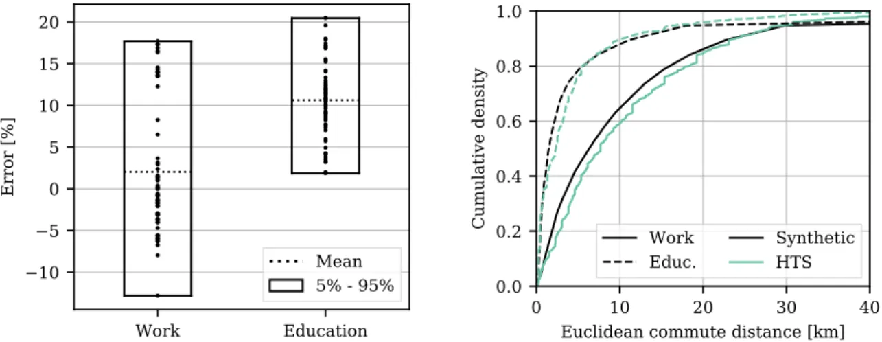
The aim of the primary location assignment is twofold: First, the correct number of people should commute from one municipality to another in the population; second, the commute distance should fit the activity chains that have been assigned to each agent in the previous step.
The synthesis step is performed in three stages. In the first stage, we iterate through all municipalities and determine how many people in the synthesized population have their home located inside of each
575
municipality k and need commuting information. Whether this is the case is determined by examining whether the person has awork oreducationactivity, respectively, in their assigned activity chain. While the following process is executed forwork andeducation commutes, we present it in general terms as the algorithm is applied independently for both activity types. The counting process results in a demand number Ok for each municipality. From the data cleaning part, we have already obtained a commuter
580
matrix, which gives a probability πk,k0. It describes the likelihood that a commute trip from origin municipality k to destination municipality k0 exists. For each origin municipality k, we can therefore sample trip countsfk,k0 ∈N+ to the destination municipalities from a multinomial distribution
(fk,1, ..., fk,·)∼Multinomial(Ok;πk,·) (7) such that in total we arrive atP
k0fk,k0 =Ok. Note that at this point, we have sampled an abstract mass of commute trips, which are not yet assigned to specific synthetic persons.
585
The second step is to find specific commute destinations for each of the sampled trips. For a combina- tion of municipalities(k, k0)we samplefk,k0 random destination candidates with replacement among all enterprises available in the destination municipality. The number of employees is used as the sampling weight. We can then define the sampled set of candidates asC(k,k0)=n
c(k,k0),1, ..., c(k,k0),f
k,k0
o.
Finally, destinations can be assigned to the synthetic population. To do so, a combined set of desti-
590
nation candidates is constructed for each home municipalityk: Ck =S
k0Ck,k0. Note that the locations in this set are still spatially distributed in a way that they resemble the commute probabilities between the municipalities. For municipality k, we can now determine all persons with a home located in that municipality and refer to them via an index u∈ {1, ..., Ok}. Likewise, we can refer to the candidates in Ck in an ordered way throughv∈ {1, ..., Ok}6. With the notation at hand, the assignment of a commute
595
destination to a person can now be described by abijective mapping A:v7→u, i.e., for each person one destination must be chosen and each destination must be chosen exactly once.
The most simple mapping isv=A(u) =u, which corresponds to a random assignment of destinations for municipality k among all inhabitants. Unfortunately, this can lead to inconsistent situations as the assigned activity chains for the persons may contain trips to work, which are very short (in terms of travel
600
time and distance from the HTS), but may still be assigned a commute destination far away. Therefore, we initially determine a commute distancefor each person uby finding the first trip in their HTS-based activity chain that takes place between a home and a work (or education, respectively) activity. After that, we denote the distance as the commute distance du ∈ R+. In some cases, agents may have work in their activity chain, but not direct trips between home and work. As the HTS does not provide
605
information about the actual locations of the activities, we assign commute distances randomly to those agents, by performing a weighted sampling among the commute distances that are known from the HTS according to the described approach.
At this point, the expected commute distanceduis known for each agent, but also the home location hu ∈R2 from the previous synthesis step. Also, the location of each destination candidate lv ∈ R2 is
610
known. We then define the destination mapping Aaccording to Algorithm 1.
6Note thatOk=|Ck|