INTRODUCTION
Definition: An antenna is an electrical conductor or system of conductors used either for
radiating electromagnetic energy into space or for collecting electromagnetic energy from space.
It is used equally for transmission and/or reception of signals materialized as radio-frequency electrical energy.
Transmission - radiates electromagnetic energy into surrounding environment:
atmosphere, space, water, etc.
Reception - collects electromagnetic energy from surrounding environment
Two-way communication, the same antenna can be used for transmission and reception
RADIATION PATTERN
An antenna radiates power in all directions but does not perform equally well in all directions. A
radiation pattern is a graphical representation of the radiation properties of an antenna as a function of space coordinates.
Graphical representation of radiation pattern of an antenna can be depicted as two-
dimensional cross section.
Omnidirectional radiation pattern produces an electromagnetic energy field of equal
strength in all directions (A and B vectors have the same length)
Directional radiation patern yields an electromagnetic energy field of different strengths
in different directions (A and B vectors have different lengths)
Idealized Radiation Patterns
Beam width (or half-power beam width) is a measure of directivity of antenna. It is the angle
within which the power radiated by the antenna is at least half of what it is in the most preffered direction
Reception pattern for a receiving antenna becomes the radiation pattern. The best direction for
reception indicates the longest section of the pattern.
TYPES OF ANTENNAS
Isotropic antenna (idealized as a point in space) radiates power equally in all directions
Dipole antennas: the half-wave dipole (Hertz antenna) and the quarter-wave vertical antenna
(Marconi antenna) are two of the simplest and most basic antennas.
Simple antennas
The Hettz-antenna consists of two straight collinear conductors of equal length, separated by a small feeding gap. The length of the antenna is ½ of the wavelength of the signal that can be transmitted most efficiently. The radiation patterns of the Hertz-antenna are represented in the next figure:
The Marconi vertical antenna is mostly used for automobile radios and portable radios.
Directional radiation pattern, with strength oriented into a given direction (next figure b) are provided by more complex antena configurations:
the wave will be reflected back in lines parallel to the axis of the paraboloid. If incoming waves are parallel to the axis the resulting signal will be concentrated at the focus. In practice there will be some dispersion. A tipical radiation patern for a parabolic reflective antenna is presented below.
Parabolic reflective antenna
Table 1. Antenna Beamwidths for Various Diameter Parabolic Reflective Antennas at f = 12 GHz [FREE97]
ANTENNA GAIN
Antenna gain (G) a measure of a directionality of an antenna. It is defined as the power output,
in a particular direction, in comparison to that produced in any direction by an ideal omnidirectional antenna. The increased power radiated in one direction is obtined by reducing the power radiated in other directions.
Effective area (Ae) a concept connected to the antenna gain, is related to physical size and
shape of antenna
Relationship between antenna gain and effective area
G = antenna gain
Ae = effective area
f = carrier frequency
c = speed of light 3 x 10⁸ m/s)
λ = carrier wavelength
Table 2. Antennas Gains and Effective Areas [COUC01]
Type of Antenna Effective
Area Ae(m2)
Power Gain (relative to isotropic) Isotropic λ2/4π 1
Infinitesimal dipole or loop 1.5 λ2/4π 1.5 Half-wave dipol 1.64 λ2/4π 1.64 Horn, mouth area A 0.81A 10A λ2 Parabolic face area A 0.56A 7A λ2 Turnstile (two crossed
perpendicular dipoles) 1.15 λ2/4π 1.15
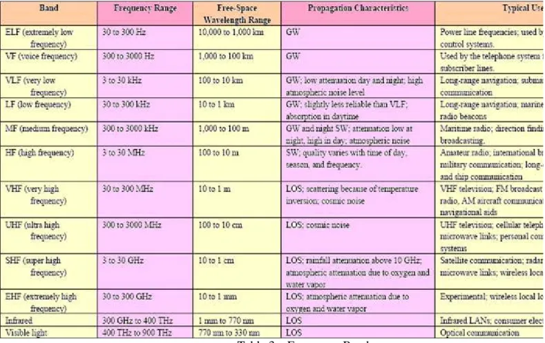
PROPAGATION MODES
Definition: A signal radiated from an antenna propagates along one of three routes and consequentelly we hav
Ground-wave propagation (GW)
Sky-wave propagation (SW)
Line-of-sight propagation (LOS)
Table 3 indicates the range of frequencies in which each predominates.
We are mainly concerned with LOS propagation, but a short overwiev of each mode is given in this section.
Table 3. Frequency Bands
1.4.1 Ground Wave Propagation
Follows contour of the earth due to the current induction in the earth’s surface and wave diffrac
frequencies (up to 2 MHz).
Can Propagate considerable distances
Example
AM radio
1.4.2 Sky Wave Propagation
Signal reflected from ionized layer of atmosphere back down to earth
Signal can travel a number of hops, back and forth between ionosphere and earth’s surface and can b
thousands of kilometers from the transmitter.
Reflection effect caused by refraction
Examples:
Transmitting and receiving antennas must be within line of sight
Satellite communication – signal above 30 MHz not reflected by ionosphere
Ground communication – antennas within effective line of site due to refraction.
1.4.4 Refraction – bending of microwaves by the atmosphere
Velocity of electromagnetic wave is a function of the density of the medium.
When wave changes medium, speed changes. In vacuum an electromagnetic wave travels at ≈ 3
constant c, commonly reffered as speed of light in a vacuum).Wave bends at the boundary between m different refractive indexes (see the next figure).
Refraction of an Electromagnetic Wave [POOL98]
The refractive index of the atmosphere decrease with heigth and radio waves travel more slowly ne
than at the higher altitudes, resulting in a slight bending of the radiowaves toward the earth.
1.4.5 Line-of-Sight Equations
Optical line of sight can be expressed as:
d = distance between antenna and horizon (km)
h = antenna height (m)
Effective, or radio, line of sight (see the next figure)
K = adjustment factor to account for refraction, rule of thumb
K = 4/3
Optical and Radio Horizons
Maximum distance between two antennas for LOS propagation:
h1 = height of antenna one
h2 = height of antenna two
LINE-OF-SIGHT WIRELESS TRANSMISSION IMPAIRMENTS
In any communication system, the signal that is received will differ from the signal that was transmitted due to various transmission impairments: random signal quality degradation, for analog signals, or bit level errors, for digital data. For LOS wireless transmission the most significant impairments are as follows:
Attenuation and attenuation distortion
Free space loss
Noise
Atmospheric absorption
Multipath
Refraction
Thermal noise
1.5.1 Attenuation
Strength of signal falls off (attenuates) with distance over transmission medium. For guided
media the attenuation is logarithmic and is expressed as a constant number in decibels (dB)/unit distance. For unguided media the attenuation is more complex function of distance and of atmosphere parameters.
Attenuation factors for unguided media:
Received signal must have sufficient strength so that circuitry in the receiver can
interpret the signal
Signal must maintain a level sufficiently higher than noise to be received without
error
Attenuation is greater at higher frequencies, causing distortion and so reducing
intelligibility. Remedy: equalize the attenuation across a band of frequencies by using amplifiers that have higher gain at higher frequencies.
1.5.2 Free Space Loss
In any type of wireless communication the signal disperses with distance, being spread over a larger and larger area. For sattelite communication this is the primary mode of signal loss. This form of attenuation si known as free space loss.
Free space loss, ideal isotropic antenna
Pt = signal power at transmitting antenna
Pr = signal power at receiving antenna
λ = carrier wavelength
d = propagation distance between antennas
c = speed of light (3 x10⁸ m/s)
where d and λ are in the same units (e.g., meters)
Free space loss equation can be recast:
Free Space Loss
Free space loss accounting for gain of other antennas:
Gt = gain of transmitting antenna
Gr = gain of receiving antenna
At = effective area of transmitting antenna
Ar = effective area of receiving antenna
1.5.3 Categories of Noise
For any data transmission, the received signal consists of the transmitted signal, distorted to some degree, plus unwanted signals reffered to as noise. Noise can be divided into the folloving categories:
Thermal noise, due to agitation of electrons, is uniformly distributed across the frequency spectrum and is reffered to as white noise.
Present in all electronic devices and transmission media
Cannot be eliminated
Function of temperature
Particularly significant for satellite communication
The amount of thermal noise, to be found in a bandwidth of 1Hz in any device or conductor, is:
N0 = noise power density in watts per 1 Hz of bandwidth
k = Boltzmann's constant = 1.3803 x 10⁻²³ J/K
T = temperature, in kelvins (absolute temperature)
Noise is assumed to be independent of frequency
Thermal noise present in a bandwidth of B Hertz (in watts):
or, in decibel-Watts:
Intermodulation noise – occurs if signals with different frequencies share the same medium
Interference caused by a signal produced at a frequency that is the sum or difference or
multiples of the original frequencies
Crosstalk – unwanted coupling between signal paths
Impulse noise – irregular pulses or noise spikes
Short duration and of relatively high amplitude
Caused by external electromagnetic disturbances, or faults and flaws in the
communications system
1.5.4 System Performance
Ratio of signal energy per bit, Eb, to noise power density per Hertz, N0, is the standard quality
measure for digital communication system performance:
S = signal power = Eb/Tb [W]
Tb = time required to send one bit
R = 1/Tb data rate
k = Boltzmann's constant = 1.3803 x 10⁻²³ J/K
T = temperature, in kelvins (absolute temperature)
or in dB notation:
(Eb/Tb)dB = SdBW – 10 log R -10 log k – 10 log T
= SdBW – 10 log R -228.6dBW – 10 log T
The bit error rate for digital data is a function of Eb/N0
Given a value for Eb/N0 to achieve a desired error rate, parameters of this formula can
be selected
As bit rate R increases, transmitted signal power must increase to maintain required
Eb/N0
1.5.5 Other Impairments
Atmospheric absorption – water vapor and oxygen contribute to attenuation. Peak attenuation
due to water vapor in the vicinity of 22 GHz., while oxygen molecules produce an peak absorbtion in the neighborhood of 60GHz. Rain and fog cause scattering of radiowaves that result in attenuation
Multipath – obstacles reflect signals so that multiple copies with varying delays are received:
Examples of Multipath Interference
Refraction – bending of radio waves as they propagate through the atmosphere
FADING IN THE MOBILE ENVIRONMENT
Fading reffers to the time variation of the received signal power caused by changes in the transmission medium or paths. The most challenging technical problem facing communications systems is fading in a mobile environment. In a fixed transmission environment fading is generated by atmospheric changes, while in a changing environment one of the two antennas is moving relative to the other, with different in time reflecting obstacles around them.
1.6.1 Multipath Propagation
The following figure illustrates three propagation mechanisms: Reflection, Diffraction and Scattering.
Sketch of Three Important Propagations Mechanisms:
Reflection (R), Diffraction (D), Scattering (S) [ADE95]
Reflection - occurs when a signal encounters a surface that is large relative to the wavelength of
the signal. The reflected waves may interfere constructively or distructively at the receiver
Diffraction - occurs at the edge of an impenetrable body that is large compared to wavelength of
radio wave
Scattering – occurs when incoming signal hits an object whose size in the order of the
wavelength of the signal or less. Scattering effects are difficult to predict.
One or more delayed copies, with different magnitudes, of a pulse may arrive at the same time as the primary pulse for a subsequent bit.
Two Pulses in Time-Variant Multipath.
This makes it difficult to design signal processing techniques that will filter out
multipath effects in order to recover the desired signal.
1.6.3 Types of Fading
Fading effects in a mobile environment can be classified as follows:
Fast fading
Slow fading
Flat fading
Selective fading
Rayleigh fading
Rician fading
Fast fading
As a mobile unit moves in an urban environment , rapid variations occur in signal strength over distances of about λ/2. At a frequency of 900MHz (mobile cellular applications) λ = 0.33 m (see the following figure). Changes in amplitude can be as much as 20- 30 dB over a short distance.
Typical Slow and Fast Fading in an Urban Mobile Environment
Slow fading
As the mobile unit covers distances well in excess of λ, the urban environment changes affecting the average received power level.
Flat fading
In tis type of fading all frequency components of the received signal are affected in the same proportion simultaneously.
Selective fading.
Affects unequally the different spectral components of a radio signal.
Rayleigh fading
This type of fading occurs when there are multiple indirect paths between transmitter and receiver and there is no a distinct dominant path, such as an LOS path (outdoor settings). It embodies the worst-case scenario.
Theoretical Bit Error Rate for Various Fading Conditions.
Rician fading.
A situation where there is a a direct LOS path in addition to a number of indirect multipath signals. This model is applicable in an indoor environment.
Forward error correction is applicable when the transmitted signal carries digital data or digitized voice or video data.
Transmitter adds error-correcting code to data block. Code is a function of the data
bits.
Receiver calculates error-correcting code from incoming data bits. If calculated
code matches incoming code, no error occurred. If error-correcting codes don’t match, receiver attempts to determine bits in error and correct
Adaptive Equalization can be applied to transmissions that carry analog voice/ video or digital
data, digitized voice or video and it is used to combat intersymbol interference.
Used to combat intersymbol interference
Involves gathering dispersed symbol energy back into its original time interval
Techniques:
- Lumped analog circuits
- Sophisticated digital signal processing algorithms (see the next figure)
Linear Equalizer Circuit [PROA01]
Diversity Techniques. Diversity is based on the fact that individual channels experience
independent fading events. The error effects can be compensated by providing multiple logical channels in some sense between transmitter and receiver and sending part of the signal over each channel. There are several types of diversities:
Space diversity – techniques involving physical transmission path. For example,
multiple nearby antennas may be used to receive the mesages, with signals combined in order to reconstruct the most likely transmitted signal.
Frequency diversity – techniques where the signal is spread out over a larger frequency
bandwidth or carried on multiple frequency carriers (e.g. spread spectrum).
Time diversity – techniques aimed at spreading the data out over time so that a noise
burst affects fewer bits. This concept is materialized in a technique called Time Division Multiplex (TMD) as in the next figure. In a slow fading condition the user A is exposed to a long burst of errors which can’t be corrected by using error correction codes.
In a TMD environment multiple users share the same phisycal channel by the use of interleaved time slots. In this case the same number of bits are affected, but they are spread out over a number of logical channels, which can be handled by error correcting codes.
If TMD is not used, the concept can still be applied by breaking the bit source stream in blocks and the shuffling the blocks.
Interleaving Data Blocks to Spread the Effects of Error Bursts
LITERATURE
BERT00 Bertoni,H. Radio Propagation for Modern Wireless Systems.
Upper Saddle River, NJ: Prentice Hall 2000.
FREE97 Freeman, R. Radio Systems Design for Telecommunications.
New York: Wiley, 1997.
STAL01 Stallings, W. Wireless Communications and Networks.
Upper Saddle River, NJ: Prentice Hall 2001.
THUR00 Turwachter, C. Data and Telecommunications: Systems and Applications.
Upper Saddle River, NJ: Prentice Hall 2000.
REVIEW QUESTIONS
1. What two functions are performed by an antenna?
2. What is an isotropic antenna?
3. What information is available from a radiation pattern?
4. What is the advantage of a parabolic reflective antenna?
5. What factors determine antenna gain?
6. What is the primary cause of signal loss in satellite communications?
7. Name and briefly define four type of noise
8. What is refraction?
9. What is fading?
10. What is the difference between diffraction and scattering?
11. What is the difference between fast and slow fading?
12. What is the difference between flat and selective fading?
13. Name and briefly define three diversity techniques.
SOLVED PROBLEMS
1. For a parabolic reflective antenna with a diameter of 2 m, operating at 12 GHz, what is the effective area and antenna gain?
Solution:
- Area: A = πr2 = π
- Effective Area: Ae = 0.56π
- Wavelength: λ = c/f = (3.108) /(12 .109) = 0.025 m
Then - G = (7A)/ λ2 = (7. π)/(0.025)2 = 35,186 - GdB = 45.46 dB
2. What is the maximum distance, d, between two antennas for LOS transmission if one antenna is 100m high and the other is at ground level?
Solution:
- K = 4/3 (empirically)
- d = 3.57√Kh = 3.57 √133 = 41 km.
3. Suppose that the receiving antenna from the previous problem is 10 m high. To achieve the same distance, d, how high must the transmitting antenna be?
Solution:
- 41 = 3.57(√Kh1 + √13.3 )
- h1 = 46.2 m
4. Determine the isotropic free space loss at 4 GHz for the shortest path to a synchronous sattelite from earth (35,836 km).
Solution:
- At 4 GHz : λ = c/f = (3.108) /(4 .109) = 0.075 m
- LdB = -20 log(0.075) + 20 log(35.853 x 10⁶) + 21.98 = 195.6 dB
Consider the antenna gain of both the sattelite and ground based antennas. Typical values are 44 dB and 48 dB, respectively. The free space loss is:
- LdB = 195.6 - 44 – 48 = 103.6 dB
Assuming a transmit power of 250 W ( 24 dBW) at the earth station, the power received at the satellite antenna is:
24 – 103.6 = -79.6 dBW.
4. Calculate the thermal noise power at room temperature T = 170 C or 290 K.
Solution:
- N0 = (1.3803 x 10-23) x 290 = 4 x 10-21 W/Hz = -204 dBW/Hz
5. Given a receiver with an effective noise temperature of 294 K, and a 10 MHz bandwidth, find the value of the thermal noise at the receiver’s outputs.
Solution:
- N = -228.6 dBW + 10 log(294) + 10 log 107 = - 133.9 dBW
6. Suppose a signal encoding technique requires that Eb/N0 = 8.4 dB for a bit error rate of 10-4 (one bit error out of every 10,000). If the effective noise temperature is 290 K (room temperature) and the data rate is 2400 bps, what received signal level is required to overcome thermal noise?
Solution:
- 8.4 = SdBW – 10 log 2400 + 228.6 dBW – 10 log 290
- SdBW = -161.8 dBW
7. Find the minimum Eb/N0 required to achieve a spectral efficiency (C/B) of 6 bps/Hz.
Solution:
INTRODUCTION
In a communications system, data are propagate from one point to another by means of electric analog or digital signals.
Analog signals represent data with continuously varying electromagnetic wave:
Digital signals represent data with sequence of voltage pulses:
Analog and Digital Signaling of Analog and Digital Data
The different encoding techniques and reasons for choosing encoding techniques are:
Digital data, digital signal: equipment less complex and expensive than digital-to-analog
modulation equipment
Analog data, digital signal: permits use of modern digital transmission and switching equipment
Digital data, analog signal: some transmission media will only propagate analog signals (e.g.,
optical fiber and unguided media)
Analog data, analog signal: analog data in electrical form can be transmitted easily and cheaply;
done with voice transmission over voice-grade lines
The following figure suggests the above mentioned encoding and modulation techniques:
Encoding /Modulation Techniques
SIGNAL ENCODING CRITERIA
Factors that determine how successful a receiver will be in interpreting an incoming signal:
Signal-to-noise ratio (SNR): an increase in SNR decreases bit error rate
Data rate: an increase in data rate increases bit error rate (BER)
Bandwidth: an increase in bandwidth allows an increase in data rate
Factors Used to Compare Encoding Schemes
Signal spectrum
- With lack of high-frequency components, less bandwidth required
- With no dc component, ac coupling via transformer possible
- Transfer function of a channel is worse near band edges
Clocking
- Ease of determining beginning and end of each bit position
Signal interference and noise immunity
- Performance in the presence of noise
Cost and complexity
- The higher the signal rate to achieve a given data rate, the greater the cost
Key Data Transmission Terms
Term Units Definition
Data element Bits A single binary one or zero
Data rate Bits per second (bps) The rate at which data elements are transmitted Signal element Digital: a voltage pulse of
constant amplitude.
Analog: a pulse of constant frequency, phase, and amplitude
That part of a signal that occupies the shortest interval of a signaling code
Signaling rate or
modulation rate
Signal elements per second (baud)
The rate at which signal elements are transmitted
DIGITAL TO ANALOG SIGNALS
ENCODING / MODULATION TECHNIQUES
The most use of this transformation is for transmitting digital data through the public telephone network (PTN). For PTN modems are used that produce signals in the voice frequency range (300 – 3400Hz).
Modulation involves operation on one or more of the three characteristics of a carrier signal: amplitude, frequency and phase:
- Amplitude-shift keying (ASK): amplitude difference of carrier frequency
- Frequency-shift keying (FSK)- most common binary frequency-shift keying (BFSK) - :
frequency difference near carrier frequency
- Phase-shift keying (PSK): phase of carrier signal shifted
-
Modulation of Analog Signals for Digital Data CALL TUTORIAL
2.2.1 Amplitude-Shift Keying (ASK)
One binary digit is represented by presence of carrier signal, at constant amplitude, Acos(2πfct), while the other binary digit is represented by absence of carrier:
Acos(2πfct) binary 1
ASK 0 binary 0
ASK is susceptible to sudden gain changes and is rather inefficient modulation technique. On voice-grade lines, used up to 1200 bps. It is used to transmit digital data over optical fiber.
( )
⎪⎩⎪⎨
= ⎧ t s
a) Binary Frequency-Shift Keying (BFSK)
Two binary digits represented by two different frequencies f1 and f2, near the carrier frequency fc.
Acos(2πf1t) binary 1
BFSK Acos(2πf2t) binary 0
This techniques is less susceptible to error than ASK. On voice-grade lines it used up to 1200 bps, while for high-frequency radio transmission it is used in the range of 3 to 30 MHz. It can be used at higher frequencies on LANs that use coaxial cable.
The next figure gives an example of the use of FSK for full-duplex (transmission in both direction simultaneously) operation over a voice-grade line.
Full-Duplex FSK Transmission on a Voice-Grade Line
b) Multiple Frequency-Shift Keying (MFSK)
MFSK assumes the usage of more than two frequencies. It is more bandwidth efficient but more susceptible to error. The transmitted MFSK signal for one signal element time is defined as follows:
MFSK
where:
- f i = f c + (2i – 1 – M)f d
- f c = the carrier frequency
- f d = the difference frequency
- M = number of different signal elements = 2 L
- L = number of bits per signal element
To match data rate of input bit stream, each output signal element is held for:
Ts = LT seconds
where T is the bit period (data rate = 1/T)
So, one signal element, a constant-frequency tone, encodes L bits. The total bandwidth required is:
2Mfd
Minimum frequency separation required:
( )
⎪⎩⎪⎨
= ⎧ t s
( )
t A ftsi = cos2π i 1≤i≤M
2fd = 1/Ts
Therefore, modulator requires a bandwidth of:
Wd =2L/LT = M/Ts
The subsequent figure shows an example of MFSK with M=4, where an input stream is encoded 2 bits at a time, with each of the four possible 2-bit combinations transmitted as a different frequency.
MFSK Frequency Use (M = 4)
CALL TUTORIAL
2.2.3 Phase-Shift Keying (PSK)
a) Two-level PSK (BPSK)
BPSK uses two phases to represent binary digits:
binary 1
BPSK binary 0
or
s(t) = A d(t) cos(2πfct)
if for a given stream of bits a discrete function d(t) is defined such that it takes on the value +1 for one bit time if the corresponding bit in the stream is 1 and the value -1 for one bit time if the corresponding bit in the stream is 0.
b) Differential PSK (DPSK)
Phase shift with reference to previous bit (see the next figure):
- binary 0 – signal burst of same phase as previous signal burst
- binary 1 – signal burst of opposite phase to previous signal burst
( )
⎪⎩⎪⎨
=⎧ t
s Acos
(
2πfct) (
πf t+π)
Acos 2 c
⎪⎩
⎪⎨
=⎧ Acos
(
2πfct) (
f t)
Acos 2π c
−
More efficient use of bandwidth can be achieved if each signaling element represents more than one bit. Instead of phase shift of 180°, as allowed in PSK, QPSK uses phase shifts multiples of π/2 (90°). Thus each signal represents two bits rather than one.
11
01
QPSK 00
10
A QPSK modulation scheme in general terms is presented in the following figure:
QPSK and OQPSK Modulators
CALL TUTORIAL
The transmitted signal will be:
s(t) = (1/√2)I(t) cos2πfct - (1/√2)Q(t) sin2πfct
In the next figure is an example of QPSK coding. The combined signals have a symbol rate that is half the input bit rate.
( )
⎪ ⎪
⎩
⎪⎪ ⎨
⎧
= t s
⎟⎠
⎜ ⎞
⎝
⎛ +
2 4
cos πf t π
A c
⎟⎠
⎜ ⎞
⎝
⎛ +
4 2 3
cos πf t π
A c
⎟⎠
⎜ ⎞
⎝
⎛ −
4 2 3
cos πf t π
A c
⎟⎠
⎜ ⎞
⎝
⎛ −
2 4
cos πf t π
A c
Example of QPSK and OQPSK Waveforms
CALL TUTORIAL
c) Multilevel PSK
By using multiple phase angles with each angle having more than one amplitude, multiple signals elements can be achieved. Thus higher bit data rates can be achieved over voice-grade lines by employing more complex modulation schemes.
In general:
- D = modulation rate, baud
- R = data rate, bps
- M = number of different signal elements = 2L
- L = number of bits per signal element
2.2.4 Quadrature Amplitude Modulation (QAM)
QAM is a combination of ASK and PSK frequently used in some wireless transmission standards.
Two different signals are sent simultaneously by using two copies of the carrier frequency, one shifted by 90° with respect to the other.
M R L
D R
log2
=
=
QAM Modulator
If two - level ASK is used, then each of the two streams can be in one of two states and the combined stream can be in one of 4 = 2 x 2 states. Systems using 64 and even 256 states have been implemented.
CALL TUTORIAL
2.2.5 Performance
The bandwidth of modulated signal (BT) is the first parameter concerning the performance of various digital-to-analog modulation schemes.
ASK, PSK BT = (1+r)R
FSK BT = 2ΔF+(1+r)R
where:
- R = bit rate
- 0 < r < 1; related to how signal is filtered
- ΔF = f2 - fc = fc - f1
MPSK
MFSK
where:
- L = number of bits encoded per signal element
- M = number of different signal elements
The next table shows the ratio of data rate, R, to transmission bandwidth for various schemes:
M R R r
L
BT r ⎟⎟
⎠
⎜⎜ ⎞
⎝
⎛ +
⎟ =
⎠
⎜ ⎞
⎝
=⎛ +
log2
1 1
( )
RM M
BT r ⎟⎟
⎠
⎜⎜ ⎞
⎝
=⎛ + log2
1
Bandwidth Efficiency (R/BT) for Various Digital-to-Analog Encoding Schemes
ANALOG DATA TO ANALOG SIGNALS ENCODING / MODULATION TECHNIQUES
Modulation has been defined as the process of combining an input signal m(t) and a carrier at frequency fc to produce a signal s(t) whose bandwidth is usually centered on fc.
When only analog transmission facilities are available, digital to analog conversion is required for digital signals transmission.
In the case of analog modulation of analog signals must be stressed that:
- a higher frequency may be needed for effective transmission
- modulation permits frequency division multiplexing.
Basic Encoding Techniques for analog data to analog signal:
Amplitude modulation (AM)
Angle modulation:
- Frequency modulation (FM)
- Phase modulation (PM)
2.3.1 Amplitude Modulation (AM)
Amplitude modulation (AM), the simplest form of modulation, mathematically can be expressed as:
s(t) = [1 + na x(t)] cos2πfct AM
where:
- cos2πfct = carrier
- x(t) = input signal
- na = modulation index (ratio of amplitude of input signal to carrier)
The “1”, in the above equation, is the dc component that prevents loss of information, when na = 1 (the envelope of the carrier frequency signal will cross the time axis).
This scheme of modulation is called: double sideband transmitted carrier (DSBTC).
The spectrum consists of the original carrier plus the spectrum of the input signal translated
to fc as in the following figures:
Spectrum of modulating signal
Spectrum of AM signal with carrier at fc
Spectrum of an AM Signal CALL TUTORIAL
Transmitted power:
- Pt = total transmitted power in s(t)
- Pc = transmitted power in carrier.
The parameter na should be as large as possible (but na < 1) so that the most of the signal power to be used to carry information.
Single Sideband (SSB)
Is a variant of AM which sends only one sideband and eliminates other sideband and carrier.
Advantages:
- Only half the bandwidth is required
- Less power is required
Disadvantages:
- Suppressed carrier can’t be used for synchronization purposes. A compromise is Vestigial Sideband (VSB) which uses only one sideband and reduced-power carrier.
2.3.2 Angle Modulation
Frequency modulation (FM) and phase modulation angle modulation (PM) are special cases of angle modulation which is expressed mathematically as:
Phase modulation (PM)
Phase is proportional to modulating signal:
⎟⎟⎠
⎞
⎜⎜⎝
⎛ +
= 1 2
2 a c t
P n P
( )
t A[
f t( )
t]
s = ccos2π c +φ
( )
t =npm( )
tφ
Frequency modulation (FM)
Derivative of the phase is proportional to modulating signal:
- nf = frequency modulation index
The peak deviation ΔF can be evaluated as:
ΔF = (1/2π) nf Am Hz,
where Am is the maximum value of m(t). Hence na increase of m(t) will also increase the transmitted signal bandwidth, but the power level of the FM signal will not be affected because this is given by: A2c/2
Compared to AM, FM and PM result in a signal whose bandwidth:
is also centered at fc
but has a magnitude that is much different and angle modulation includes cos(φ(t))
which produces a wide range of frequencies like fc + fm, fc + 2 fm etc. Thus, FM and PM require greater bandwidth than AM, for which:
BT = 2B
For PM and FM the Carson’s rule can be used in order to estimate the necessary BT:
where:
The formula for FM becomes
( )
t =nfm( )
t φ'( )
BBT =2 β+1
FM for
PM for
⎪⎩ 2
⎪⎨
⎧ Δ =
=
B A n B
F A n
m f m p
π β
B F BT =2Δ +2
ANALOG DATA TO DIGITAL SIGNALS ENCODING / MODULATION TECHNIQUES
The process of transforming analog data into digital signal is known as digitization.
Once analog data have been converted to digital signals, the digital data:
can be transmitted using NRZ-L
can be encoded as a digital signal using a code other than NRZ-L
can be converted to an analog signal, using previously discussed techniques as in the
following figure:
Digitizing Analog Data
Note: NRZ-L (none return to zero – level) is the most simple and easiest method to transmit digital signals. It uses two different voltage levels for transmitting the two binary digits. A negative voltage represents binary 1, while a positive voltage level represents binary 0.
A device used for converting analog data into a digital form for transmission and subsequently recovering the original analog data from the digital, is known as a codec(coder-decoder).
The principal two techniques used in codecs are:
Pulse code modulation (PCM)
Delta modulation (DM)
2.4.1 Pulse Code Modulation (PCM)
PCM is based on the sampling theorem, which states as follows:
If a signal f(t) is sampled at regular intervals of time and at a rate higher than twice the highest signal frequency, then the samples contain all the information of the original signal. the function f (t) may be reconstructed from these samples by using a low- pass filter.
PAM value 1.1 9.2 15.2 10.8 5.6 2.8 2.7 Quantized 1 9 15 10 5 2 2 code number
PCM code 0001 1001 1111 1010 0101 0010 0010
Pulse Code Modulation
By quantizing the PAM pulse, original signal is only approximated. The approximation error depends on the number of quantizing levels. This aspect generates the quantizing noise.
The signal-to-noise ratio (SRN) for quantizing noise can be expressed as:
Thus, each additional bit increases SNR by 6 dB, or a factor of 4
Nonlinear encoding. The PCM scheme is refined by using a technique known as nonlinear
encoding , which means that the quantization levels are not equally spaced. An overall signal distortion reduction, and especially for signals of low amplitude, is achieved by using more quantizing steps for signals of low amplitude than for signals of high amplitude (see the next figure).
Effect of Nonlinear Coding
Nonlinear encoding can improve the PCM SNR ratio significantly: 24-30 dB, for voice signals.
Companding (compressing-expanding). Companding (next figure) is a process that
compresses the intensity range of a signal by imparting more gain to weak signals than to strong signal on input. At output, the reverse operation is performed. Thus with a fixed number of quantizing levels, more levels are available for lower-level signals.
In the case of Delta Modulation the analog input is approximated by a staircase function that moves up or down by one quantization level (δ) at each sampling interval (Ts).
The bit stream approximates derivative of analog signal (rather than amplitude):
- 1 is generated if function goes up
- 0 otherwise
Example of Delta Modulation
The two important parameters are:
- Size of step assigned to each binary digit (δ)
- Sampling rate 1/Ts
The accuracy is improved by increasing sampling rate. However, this increases the data rate.
Advantage of DM over PCM is the simplicity of its implementation.
The following figure presents the transmission and reception for DM technique.
Delta Modulation
2.4.2 Performance
With 128 quantization levels or 7- bit coding (27 = 128) a good voice reproduction via PCM can be achieved. A voice signal occupies a bandwidth of 4 kHz, so samples should be taken at a rate of 8000 samples/sec. This implies a data rate of 8000 x 7 = 56 kbps, for the PCM – encoded analog signal, signal which occupies 4 kHz.
A common PCM scheme for color television uses 10 – bit codes, which work out to 92 Mbps for a 6.6 MHz bandwidth signal.
In spite of these results there is a growth in popularity of digital techniques for transmitting analog data because:
- repeaters are used instead of amplifiers, which means no additive noise,
- Time Division Multiplexing (TDM) is used instead of Frequency Division
Multiplexing (FDM), leading to intermodulation noise absence,
- conversion to digital signaling allows use of more efficient digital switching
techniques.
LITERATURE
COUC10 Couch, L. Digital and Analog Communication Systems.
Upper Saddle River, NJ: Prentice Hall 2001.
FREE97 Freeman, R. Bits, Symbols, Baud, and Bandwidth.
IEEE Communications Magazine, April 1998.
GLOV98 Glover, I., and Grant, P. Digital Communications.
Upper Saddle River, NJ: Prentice Hall 1998.
PEAR92 Pearson, J. Basic Communication Theory. Engelwood Cliffs.
NJ:Prentice Hall, 1992.
SKLA93 Sklar, B. Defining, Designing, and Evaluating Digital Communication Systems. IEEE Communications Magazine, November 1993.
SKLA93 Sklar, B. Digital Communication Fundamentals and Applications.
Upper Saddle River, NJ: Prentice Hall 2001.
STAL01 Stallings, W. Wireless Communications and Networks.
Upper Saddle River, NJ: Prentice Hall 2001.
XION00 Xiong, F. Digital Modulation Techniques, Boston: Artech House, 2000.
THUR00 Turwachter, C. Data and Telecommunications: Systems and Applications.
Upper Saddle River, NJ: Prentice Hall 2000.
REVIEW QUESTIONS
1. What is differential encoding?
2. What function does a modem perform?
3. Indicate three major advantages of digital transmission over analog transmissioNn
4. How are binary values represented in amplitude shift keying, and what is the limitation of this approach?
5. What is NRZ-L? What is a major disadvantage of this data encoding approach?
SOLVED PROBLEMS
1. Consider the MFSK modulation technique with fc = 250 kHz, fd = 25 kHz, and M = 8 (L =
3). Establish the frequencies assignment for each of the 8 possible 3 – bit data combinations, and data rate supported.
Solution:
The transmitted MFSK signal for one signal element time is defined as follows:
MFSK
where:
- f i = f c + (2i – 1 – M)f d
- f c = the carrier frequency
- f d = the difference frequency
- M = number of different signal elements = 2 L
- L = number of bits per signal element
So:
f1 = 75 kHz 000 f2 = 125 kHz, 001 f3 = 175 kHz 010 f4 = 225 kHz, 011
f5 = 275 kHz 100 f6= 325 kHz, 101 f7 = 375 kHz 110 f8 = 425 kHz, 111
Data rate:
2fd = 1/Ts = 50 kbps.
2. What is the bandwidth efficiency for FSK, ASK, PSK, and QPSK for a bit error rate of 10-7
on a channel with an SNR of 12 dB?
Solution:
Remember, from a former chapter, that the ratio of signal energy per bit, Eb, to noise power density per Hertz, N0, is the standard quality measure for digital communication system performance:
where:
- S = signal power = Eb/Tb [W]
- Tb = time required to send one bit
- R = 1/Tb data rate
- k = Boltzmann's constant = 1.3803 x 10⁻²³ J/K
- T = temperature, in kelvins (absolute temperature)
or in dB notation:
(Eb/Tb)dB = SdBW – 10 log R -10 log k – 10 log T
= SdBW – 10 log R -228.6dBW – 10 log T
The noise in a signal with bandwidth BT si N = N0BT and substituting we have:
Eb/N0 = (S/N).(BT/R) In this case:
(Eb/N0)dB = 12 dB - (R/ BT)dB
Theoretical Bit Error Rate for Various Encoding Schemes are given in the following figure:
For FSK and ASK, using the above figure, we obtain:
(Eb/N0)dB = 14.2 dB (R/ BT)dB = -2.2 dB R/ BT = 0.6
For PSK, using the above figure, we obtain:
(Eb/N0)dB = 11.2 dB (R/ BT)dB = 0.8 dB R/ BT = 1.2
The result for QPSK must take into account that the baud rate d = R/2, and thus:
R/ BT = 2.4
3. Derive an expression for s(t) if x(t) is the amplitude modulating signal cos2πfct
Solution:
We have:
The resulting signal has a component at the original carrier frequency plus a pair of components each spaced fm Hz from the carrier.
SPREAD SPECTRUM
Input is fed into a channel encoder
Result: analog signal with narrow bandwidth
Signal is further modulated using sequence of digits
Spreading code or spreading sequence
Generated by pseudonoise, or pseudo-random number generator
Effect of modulation is to increase bandwidth of signal to be transmitted
On receiving end, digit sequence is used to demodulate the spread spectrum signal
Signal is fed into a channel decoder to recover data
What can be gained from apparent waste of spectrum?
Immunity from various kinds of noise and multipath distortion
Can be used for hiding and encrypting signals
Several users can independently use the same higher bandwidth with very little
interference
FREQUENCY HOPING SPREAD SPECTRUM (FHSS)
Signal is broadcast over seemingly random series of radio frequencies
A number of channels allocated for the FH signal
Width of each channel corresponds to bandwidth of input signal
Signal hops from frequency to frequency at fixed intervals
Transmitter operates in one channel at a time
Bits are transmitted using some encoding scheme
At each successive interval, a new carrier frequency is selected
Channel sequence dictated by spreading code
Receiver, hopping between frequencies in synchronization with transmitter, picks up message
Advantages:
Eavesdroppers hear only unintelligible blips
Attempts to jam signal on one frequency succeed only at knocking out a few bits
FHSS Using MFSK
MFSK signal is translated to a new frequency every Tc seconds by modulating the MFSK signal
with the FHSS carrier signal
For data rate of R:
duration of a bit: T = 1/R seconds
duration of signal element: Ts = LT seconds
Tc ≥ Ts - slow-frequency-hop spread spectrum
Tc < Ts - fast-frequency-hop spread spectrum
FHSS Performance Considerations
Large number of frequencies used
Results in a system that is quite resistant to jamming
Jammer must jam all frequencies
With fixed power, this reduces the jamming power in any one frequency band
DIRECT SEQUENCE SPREAD SPECTRUM (DSSS)
Each bit in original signal is represented by multiple bits in the transmitted signal
Spreading code spreads signal across a wider frequency band
Spread is in direct proportion to number of bits used
One technique combines digital information stream with the spreading code bit stream using exclusive
Example of Direct Sequence Spread Spectrum
DSSS Using BPSK
Multiply BPSK signal,
sd(t) = A d(t) cos(2π fct) by c(t) [takes values +1, -1] to get s(t) = A d(t)c(t) cos(2π fct)
A = amplitude of signal
fc = carrier frequency
d(t) = discrete function [+1, -1]
At receiver, incoming signal multiplied by c(t)
Since, c(t) x c(t) = 1, incoming signal is recovered
CODE-DIVISION MULTIPLE ACCES (CDMA)
Basic Principles of CDMA
Break each bit into k chips
Chips are a user-specific fixed pattern
D = rate of data signal
Chip data rate of new channel = kD
CDMA Example
If k=6 and code is a sequence of 1s and -1s
For a ‘1’ bit, A sends code as chip pattern
<c1, c2, c3, c4, c5, c6>
For a ‘0’ bit, A sends complement of code
<-c1, -c2, -c3, -c4, -c5, -c6>
Receiver knows sender’s code and performs electronic decode function
<d1, d2, d3, d4, d5, d6> = received chip pattern
<c1, c2, c3, c4, c5, c6> = sender’s code
User A code = <1, –1, –1, 1, –1, 1>
To send a 1 bit = <1, –1, –1, 1, –1, 1>
To send a 0 bit = <–1, 1, 1, –1, 1, –1>
User B code = <1, 1, –1, – 1, 1, 1>
To send a 1 bit = <1, 1, –1, –1, 1, 1>
Receiver receiving with A’s code
(A’s code) x (received chip pattern)
User A ‘1’ bit: 6 -> 1
User A ‘0’ bit: -6 -> 0
User B ‘1’ bit: 0 -> unwanted signal ignored
![Table 1. Antenna Beamwidths for Various Diameter Parabolic Reflective Antennas at f = 12 GHz [FREE97]](https://thumb-eu.123doks.com/thumbv2/1library_info/4440527.1586197/4.892.227.661.145.797/table-antenna-beamwidths-various-diameter-parabolic-reflective-antennas.webp)