ON RULES OF THUMB FOR MONETARY POLICY

(1)

Economic Projections and Rules of Thumb for Monetary Policy

Athanasios Orphanides and Volker Wieland

Monetary policy analysts often rely on rules of thumb, such as the Taylor rule, to describe historical monetary policy decisions and to compare current policy with historical norms. Analysis along these lines also permits evaluation of episodes where policy may have deviated from a simple rule and examination of the reasons behind such deviations. One interesting question is whether such rules of thumb should draw on policymakers’ forecasts of key variables, such as inflation and unemployment, or on observed outcomes. Importantly, deviations of the policy from the prescriptions of a Taylor rule that relies on outcomes may be the result of systematic responses to information captured in policymakers’ own projections. This paper investigates this proposition in the context of Federal Open Market Committee (FOMC) policy decisions over the past 20 years, using publicly available FOMC projections from the semiannual monetary policy reports to Congress (Humphrey-Hawkins reports). The results indicate that FOMC decisions can indeed be predominantly explained in terms of the FOMC’s own projections rather than observed outcomes. Thus, a forecast-based rule of thumb better characterizes FOMC decisionmaking. This paper also confirms that many of the apparent deviations of the federal funds rate from an outcome-based Taylor-style rule may be considered systematic responses to information contained in FOMC projections. (JEL E52)

Federal Reserve Bank of St. LouisReview, July/August 2008,90(4), pp. 307-24.

can serve as a useful tool for understanding historical monetary policy decisions (Poole, 2007).

In both his recent and earlier work, Poole high- lighted the usefulness of rules of thumb in the context of the complexity of the macroeconomy and our limited knowledge regarding it. In this light, a policy adviser cannot offer precise guid- ance about how the monetary authority should respond to every conceivable contingency to best achieve its goals. What a policy adviser can do is identify useful rules of thumb that can serve as appropriate guides to policy under most circumstances. To the extent policymakers rely on

W

illiam Poole has been a long-time proponent of rules of thumb for monetary policy. Nearly four decades ago, as staff economist at the Board of Governors of the Federal Reserve System (BOG), Poole presented a reactive rule of thumb that he argued could serve as a robust guide to policy decisions (Poole, 1971). More recently, as president of the Federal Reserve Bank of St. Louis and a member of the Federal Open Market Committee (FOMC), he has high- lighted how a simple Taylor rule that systematically responds to economic activity and inflation

Athanasios Orphanides is the Governor of the Central Bank of Cyprus, and Volker Wieland is a professor at the Goethe University Frankfurt, director at the Center for Financial Studies, and fellow at the Centre for Economic Policy Research. Volker Wieland thanks the Stanford Center for International Development, where he was a visiting professor while writing this paper. The authors are grateful for excellent research assistance by Sebastian Schmidt from Goethe University Frankfurt. Helpful comments were provided by Greg Hess, Jim Hamilton, participants at the St. Louis conference, and the paper’s discussants, Charles Plosser and Patrick Minford.

©2008, The Federal Reserve Bank of St. Louis. The views expressed in this article are those of the author(s) and do not necessarily reflect the views of the Federal Reserve System, the Board of Governors, the regional Federal Reserve Banks, the Central Bank of Cyprus, or the Governing Council of the European Central Bank. Articles may be reprinted, reproduced, published, distributed, displayed, and transmitted in their entirety if copyright notice, author name(s), and full citation are included. Abstracts, synopses, and other derivative works may be made only with prior written permission of the Federal Reserve Bank of St. Louis.

(2)

a simple rule of thumb as an approximate policy guide, it should be possible to identify this rule and use it to understand historical policy decisions and to improve future policy.

One of the difficulties in identifying a simple rule that can serve as a useful description of policy is that the policy prescriptions relevant for policy advice at any point in time reflect the information available to policymakers at that time. To the extent policy is based on observable macroeconomic variables, a simple rule could be estimated using real-time historical data. However, to the extent policymakers view projections of key macroeconomic variables as more useful summary descriptions of the current state of the economy, estimation of a simple rule based on those same policymaker projections would provide a more promising avenue. Poole (2007) examines FOMC policy decisions over the past 20 years using the simple outcome-based rule proposed by Taylor (1993). This rule uses the current inflation rate and output gap as inputs for federal funds rate decisions. Poole identifies some deviations of policy from the systematic prescriptions suggested by the rule that could, however, reflect a systematic response of the FOMC to its own projections.

Our objective in this paper is to investigate this proposition. To this end we compare estimated policy rules that are based on recent economic outcomes with policy rules based on the economic projections of the FOMC. We investigate whether the federal funds rate target set by the FOMC when these projections are made responds systematically to these projections as opposed to recent economic data.

Our results, which are based on real-time data and projections over the past 20 years, indicate that interest rates respond predominantly to FOMC projections and thus that a forecast-based rule better characterizes FOMC decisionmaking during this period. Furthermore, we check to what extent deviations from an outcome-based Taylor rule may be better explained by the information incorporated in FOMC forecasts. Our analysis suggests that by distinguishing between forecasts and outcomes one can explain a number of deviations of policy from the simple underlying rule, though it can also identify episodes where devi-

ations remain. This includes episodes where one would expect systematic policy to deviate from a simple rule of thumb, such as the response to financial turbulence experienced in 1998.

Overall, our analysis suggests that FOMC projections used in the context of a rule of thumb are quite informative for understanding historical monetary policy, whereas similar analysis based on economic outcomes can often be of much lower value.

ON RULES OF THUMB FOR MONETARY POLICY

Simple estimated rules can be useful devices for understanding historical monetary policy if central banks conduct policy sufficiently systematically to be captured by such rules. Poole (1971) suggested that it is reasonable for individual policymakers to behave in a systematic manner:

Individual policy-makers inevitably use infor- mal rules of thumb in making decisions. Like everyone else, policy-makers develop certain standard ways of reacting to standard situa- tions. These standard reactions are not, of course, unchanging over time, but are adjusted and developed according to experience and new theoretical ideas. (p. 151)

Though it did not attract much attention at the time, the particular rule of thumb proposed by Poole in 1971 is of interest in that it incorporated both a reaction of the interest rate to real economic activity (specifically the deviation of the unemployment rate from the Federal Reserve’s estimate of the full employment rate at the time), as well as a nominal variable in a way that would ensure price stability over the long run. The latter was not based on the response of the interest rate to inflation, as is commonly specified today.

Rather, Poole’s rule specified that the money sup- ply should always be contained within bounds as a robust means of controlling inflation and suggested adjusting the interest rate to respond to deviations of unemployment from full employment only when doing so would respect these bounds. In essence, Poole’s rule of thumb uses money growth to ensure the maintenance of price

(3)

stability and, subject to that, provides countercyclical policy prescriptions. He provided the following summary description:

The proposed rule assumes that full employment exists when the unemployment rate is in the 4.0 to 4.4 per cent range. The rule also assumes that at full employment, a growth rate of the money stock of 3 to 5 per cent per annum is consistent with price stability. Therefore, when unemployment is in the full employment range, the rule calls for monetary growth at the 3 to 5 per cent rate.

The rule calls for higher monetary growth when unemployment is higher, and lower monetary growth when unemployment is lower. Furthermore, when unemployment is relatively high the rule calls for a policy of pushing the Treasury bill rate down provided monetary growth is maintained in the specified range; similarly, when unemployment is relatively low the rule calls for a policy of pushing the Treasury bill rate up provided monetary growth is in the specified range. Finally, the rule provides for adjusting the rate of growth of money according to movements in the Treasury bill rate in the recent past. (p. 183) Poole also explicitly recognized a scope for deviations from his suggested rule of thumb, even if policymakers had decided to adopt it in principle. What was more important in Poole’s view was transparency in explaining the rationale for such deviations:

It is not proposed that this rule of thumb or guideline be followed if there is good reason for departure. But departures should be justi- fied by evidence and not be based on vague intuitive feelings of what is needed since the rule was carefully designed from the theoretical and empirical analysis...and from a careful review of post-accord monetary policy. (p. 183) As to whether rules could usefully rely on economic projections, Poole (1971) argued that an important factor would be the accuracy of the forecasts:

Given the accuracy of forecasts at the current state of knowledge, it seems likely that for some time to come forecasts will be used pri- marily to supplement a policy-decisionmaking

process that consists largely of reactions to current developments. Only gradually will policy-makers place greater reliance on formal forecasting models. (pp. 152-53)

In 2007, Poole used a version of the classic Taylor (1993) rule to describe Federal Reserve behavior over the past 20 years.¹As is well known, this rule posits that the systematic component of monetary policy may be described as a notional target for the federal funds rate,fˆ:

(1)

whereπ^and^yreflect contemporaneous readings of inflation and a measure of the output gap, respectively. Following Taylor, Poole assumed a constant inflation target,π^*, and a constant equilibrium real interest rate,r^*. Poole’s rendition of the Taylor rule is reproduced in Figure 1.

As in his work 36 years earlier, Poole (2007) explained potential sources of deviation from the rule and also the potential use of forecasts:

The FOMC, and certainly John Taylor himself, view the Taylor rule as a general guideline.

Departures from the rule make good sense when information beyond that incorporated in the rule is available. For example, policy is forward looking, which means that from time to time the economic outlook changes sufficiently that it makes sense for the FOMC to set a funds rate either above or below the level called for in the Taylor rule, which relies on observed recent data rather than on economic forecasts of future data. Other circumstances—an obvious example is September 11, 2001—call for a policy response. These responses can be and generally are understood by the market. Thus, such responses can be every bit as systematic as the responses specified in the Taylor rule.

(p. 6)

This last remark suggests that a better rule of thumb for understanding the behavior of the Federal Reserve over the past 20 years could be a version of the Taylor rule that is explicitly based

ˆ ^* . ^* .

f = + +r ^π ^{0 5}

(

^{π π}−

)

⁺^{0 5 ,}y

1 Taylor (1993) showed that the rule could describe Federal Reserve

behavior from 1987 to 1992 quite well. Interest rate rules had also acquired a normative dimension at that time because of their success in a large-scale model comparison project reported in Bryant, Hooper, and Mann (1993) (see also Henderson and McKibbin, 1993).

(4)

on the FOMC’s own projections. This is the subject of the investigation that follows.

FOMC ECONOMIC PROJECTIONS AND REAL-TIME OUTCOMES

We begin by describing how to construct constant-horizon forecasts that can be used in estimating a policy rule from publicly available projections. The semiannual monetary policy reports to Congress (the Humphrey-Hawkins reports) have presented information on the range and central tendency of annual forecasts of FOMC members since 1979.²

Following Poole’s (2007) analysis, we create a dataset of FOMC projections and corresponding real-time data on observed outcomes that focuses our attention on the past 20 years.³

Regarding projections, we take the midpoints of the central tendencies reported in each of the reports, starting with the February 1988 report and ending with the July 2007 report, and use these as proxies for the modal forecasts of FOMC expec- tations. Our objective using these data is to examine whether deviations from an outcome-based Taylor rule may be explained by the additional information contained in policymakers’ forecasts.

These include inflation, the rate of unemployment, and output growth. Because we could not make approximate inferences of the FOMC forecasts of the output gap from these variables, although we do have the FOMC’s unemployment projections, we focus on a version of the Taylor rule that sub- stitutes the unemployment rate for the output gap.

Consequently, in our dataset we focus on data and forecasts regarding inflation and unemployment.

2 A month after this paper was first presented, on November 14, 2007,

the Federal Reserve announced that going forward the FOMC would compile and release these economic projections four times a year instead of just two times a year, which was the practice until then.

12

10

8

6

4

2

0

1986 1988 1990 1992 1994 1996 1998 2000 2002 2004

Percent

FOMC Meeting Dates

BOG Output Gap: CPI, 1987:09–2000:10 Federal Funds Rate

CBO Output Gap: CPI, 2000:11–2006:06

Figure 1

Poole’s (2007) Version of the Taylor Rule

NOTE: The solid blue line shows the Taylor rule constructed using the BOG real-time output-gap estimate. The blue dashed line extends the rule using the output-gap estimate of the CBO for those years for which the BOG estimate is not yet public information.

3 In earlier work, Lindsey, Orphanides, and Wieland (1997), we

examined the implications of FOMC projections for understanding policy in the sample prior to 1988 and presented some comparisons with the 1988-96 period.

(5)

Some of the particular measures have been redefined over the years. For inflation, the implicit deflator of the gross national product was used through July 1988, thereafter replaced by the con- sumer price index (CPI). In February 2000, the CPI was replaced by the personal consumption expenditures (PCE) deflator measure of inflation, and from July 2004 onward the FOMC decided to focus on the core PCE deflator that excludes food and energy prices because of their volatility. These changes are of particular interest because the alternative measures do not always provide similar summary readings of inflationary pressures.

They may differ both in their level and in their variability over time, especially in small samples, which poses some interpretation challenges.

Tables 1 and 2 provide two recent examples useful for understanding what information on projections is released with the monetary policy reports. Forecasts for 2007 were first reported in July 2006 (not shown). In February 2007, revised forecasts for 2007 and first forecasts for 2008 were reported (Table 1). The final updated forecasts for 2007 were then published in July together with updated forecasts for 2008 (Table 2).

Although we have only two observations per year, it is convenient to describe our dataset in

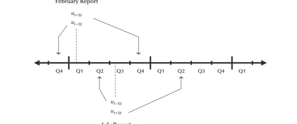
terms of a quarterly frequency because the FOMC projections report either quarterly data or growth rates over four quarters. Denoting time (measured in quarters) witht, we associate the February Humphrey-Hawkins report with the first quarter of the year and the July Humphrey-Hawkins report with the third quarter. We construct a dataset con- taining two sets of forecasts for each year, cover- ing four-quarter intervals that always end three quarters in the future. For any variablex, letx_t_+i|t denote the estimated outcome (foriⱕ0) or forecast (fori> 0) of the value of the variablexatt+i as of timet.⁴Then, lettingudenote the unemployment rate,u_t_+3|trepresents the three-quarter-ahead forecast of the unemployment rate formed during quartert, andu_t_–1|_tthe estimate as of quartertof what the outcome for the unemployment rate was in the previous quarter.

As shown on the time chart in Figure 2, using the unemployment rate as an example, the forecasts reported to Congress in the February

4 Importantly, because of the lags with which information about the

past becomes available, we need to keep track not only of revisions of forecasts but also of revisions regarding outcomes when trying to understand the environment in which FOMC decisions were taken. We later describe the data we use for outcomes.

Q4 Q1 Q2 Q3 Q4 Q1 Q2 Q Q Q1

February Report

July Report

3 4

u_t+3|t^HH

u_t+1|t^HH u_t+3|t^HH u_t+5|t^HH

Figure 2

The Timing of Forecasts in Humphrey-Hawkins Reports: Unemployment Rates

(6)

Table 1

FOMC Forecasts for 2007 and 2008 from the February 2007 Humphrey-Hawkins Report

2007 2008

Indicator Memo 2006 actual Range Central tendency Range Central tendency Change, fourth quarter to fourth quarter*

Nominal GDP 5.9 4³/4–5¹/2 5–5¹/2 4³/4–5¹/2 4³/4–5¹/4

Real GDP 3.4 2¹/2–3¹/4 2¹/2–3 2¹/2–3¹/4 2³/4–3

PCE price index excluding food and energy 2.3 2–2¹/4 2–2¹/4 1¹/2–2¹/4 1³/4–2 Average level, fourth quarter

Civilian unemployment rate 4.5 4¹/2–4³/4 4¹/2–4³/4 4¹/2–5 4¹/2–4³/4

NOTE: *Change from average for fourth quarter of previous year to average for fourth quarter of year indicated.

SOURCE: “Economic Projections of Federal Reserve Governors and Reserve Bank Presidents” from the February 2007 Humphrey- Hawkins report.

Table 2

FOMC Forecasts for 2007 and 2008 from the July 2007 Humphrey-Hawkins Report

2007 2008

Indicator Range Central tendency Range Central tendency

Change, fourth quarter to fourth quarter*

Nominal GDP 4¹/2–5¹/2 4¹/2–5 4¹/2–5¹/2 4³/4–5

Real GDP 2 –2³/4 2¹/4–2¹/2 2¹/2–3 2¹/2–2³/4

PCE price index excluding food and energy 2–2¹/4 2–2¹/4 1³/4–2 1³/4–2 Average level, fourth quarter

Civilian unemployment rate 4¹/2–4³/4 4¹/2–4³/4 4¹/2–5 About 4³/4

NOTE: *Change from average for fourth quarter of previous year to average for fourth quarter of year indicated.

SOURCE: “Economic Projections of Federal Reserve Governors and Reserve Bank Presidents” from the July 2007 Humphrey-Hawkins report.

(7)

Humphrey-Hawkins report have exactly the desired timing. That is, whentis the first quarter, the three-quarter-ahead forecast of unemployment,

u_t+3|t, corresponds to the February Humphrey-

Hawkins forecast of the unemployment rate in the fourth quarter of the same year. That is, when trepresents the first quarter of a year, we have (2)

where we employ the superscriptHHto denote the Humphrey-Hawkins forecasts.

Note that in Figure 2 under the heading

‘‘February Report” the solid arrow points to the quarter on the time line for which the unemployment rate is predicted (t+3) and the dotted line points to the quarter in which the forecast is made (t). Similarly, for inflation, whentrepresents the first quarter of a year, the three-quarter-ahead forecast corresponds to the rate of growth of prices from the fourth quarter of the previous year to the fourth quarter of the current year, exactly match- ing the horizon of the February Humphrey- Hawkins forecast. Lettingπrepresent the rate of inflation over four quarters, whentis the first quarter of a year, we have

(3)

For the July Humphrey-Hawkins reports, some additional work is required to obtain three- quarter-ahead projections; that is, we combine available information to estimate the forecast of the unemployment rate for the second quarter of next year and the corresponding forecast of the four-quarter growth rate of prices that ends in the same quarter. The timing of the two July Humphrey-Hawkins forecasts and the constructed three-quarter-ahead unemployment forecast is also shown with respect to the time line in Figure 2.

In this case, the dashed arrow refers to the three- quarter-ahead observation for which an unemployment forecast is needed. To approximate the unemployment forecast for the second quarter of the following year, we simply take from the July Humphrey-Hawkins report the forecasted unemployment rates for the current year’s fourth quarter and next year’s fourth quarter and average them.

That is, whentrepresents the third quarter of the year, we set

π^t₊³^|^t^;π^t^HH₊³^|^t^. u_t₊₃_|_t _;u_t^HH₊₃_|_t,

(4)

Other than the rare occurrence of when a shock is known to have only transitory effects, for a four-quarter interval that starts two quarters later, it is doubtful that FOMC members would have strong views about the likelihood of different changes in the unemployment rate over the two halves of that period. Implicitly, we assume that the changes forecasted in July for the unemployment rate in each half of next year are about the same.

The desired second-quarter-to-second-quarter forecasts of the growth rate of prices is obtained by constructing two forecasted half-year annualized growth rates and then averaging them. In other words, whentrepresents the third quarter of the year, we set

(5)

whereSstands for semiannual, so thatπ^S^t+1|t^is the inflation forecast for the second half of the current year andπ^t^S^+3|^tis the forecast for the first half of the following year.

The inflation forecasted for the second half of the current year,π^t^S^+1|^t, can be inferred from the forecast reported for all of the year from a base of last year’s fourth quarter,πt+1|t^HH , and the estimated inflation over the first half of the current year from a base of last year’s fourth quarter,π^t^S^–1|t^{. That is,} expressing all terms as annualized growth rates, whentrepresents the third quarter of the year, (6)

Forπ^S^t+3|t, inflation over the first half of the

next year, we simply set it equal to the July Humphrey-Hawkins forecast for all of next year.

That is, we set (7)

The July Humphrey-Hawkins report does not provide an estimate of inflation for the first half of the current year, that is, forπ^S^t–1|t. Thus, instead we make use of alternative real-time data sources, which are discussed below.

π^t^S+³^|^t =π^t^HH+⁵^|^t. πt t π π

S

t t

HH

t t

S +¹_| =2 +¹_| − −¹_|. π^t₊³^|^t =¹2

(

π^t^S₊¹^|^t +π^t^S₊³^|^t

)

, u_t₊³^|_t =¹2

(

u_t^HH₊¹^|_t+u_t^HH₊⁵^|_t

)

.

(8)

To allow for a direct comparison of rules based on the forecasts described above with rules based on outcomes of these variables, we construct parallel variables reflecting the latest historical information available to the FOMC at the time of their meetings preceding the two Humphrey- Hawkins reports each year.

Thus, for the unemployment rate, we create the variableu_t–1|t, which for the February observation reflects the average level in the fourth quarter of the prior year and for the July observation reflects the average level in the second quarter of the current year. Similarly, for inflation, we create the variableπ^t^–1|^t, which reflects the four-quarter growth rate of prices ending in the fourth quarter of the prior year for the February observation and ending in the second quarter of the current year for the July observation.

An important aspect of our analysis is to ensure that our definition of outcomes reflects only information available to the FOMC in real time. To that end, we rely only on data that would have been available to the FOMC by early February or early July. This implies that the data we use correspond either to preliminary estimates, first- reported quarterly data, or estimates based on partial data for the quarter.

To match the timing of this information as closely as possible, for the years 1988 through 2001 inclusive, we use BOG staff estimates of outcomes ending in the prior quarter, which are contained in theGreenbookthat is distributed to the FOMC prior to the early-February and early- July FOMC meetings. Even so, becauseGreenbook data remain confidential for five years, we cannot rely on that source for the last few years of our sample. Instead, for 2002-07 we use real-time vintage data from the Federal Reserve Bank of St. Louis ALFRED database.⁵For these dates we use the data vintage from ALFRED that was available one week after the respective February and July Humphrey-Hawkins meetings. We choose this timing because FOMC members have the

opportunity to revise their projections during a window of a few days following the meetings.

ESTIMATED POLICY RULES:

FOMC PROJECTIONS VERSUS RECENT OUTCOMES

Specification

The interest rate rules we estimate all share the following underlying structure with Taylor’s (1993) rule. They posit that the systematic component of monetary policy can be described as a notional target for the federal funds rate,fˆ, which increases with inflation,π, and real activity.

As already mentioned with regard to projections of real activity, we do not have information about the FOMC’s assessment of the output gap.

Thus, we cannot directly estimate an exact coun- terpart of the rule proposed by Taylor. Instead, an indirect comparison is feasible using the unemployment rate,u, as a measure of the level of economic activity.⁶

Following Taylor, we restrict attention to a linear specification of the rule and posit that⁷ (8)

Note that we do not have direct information on the policymakers’ views regarding the equilibrium interest rate,r^*, the inflation target,π^*^{, or the} natural rate of unemployment,u^*. If these concepts are roughly constant over the sample period, then they would be subsumed in the estimated intercept,

In estimating our specification, we need to take an explicit stand regarding the explanatory

a₀ = −r^*

(

a^π −1

)

^π^*⁻a u_u ^*^. fˆ= +a⁰ a_ππ+a u_u ^.

5 As a robustness check, we have investigated how much the

ALFRED-based information differs fromGreenbookinformation in the years until 2001, when both are available. Although the data source does influence the data values somewhat, the differences were small.

6 The difference between the unemployment rate and a constant

natural rate (NAIRU) can then be translated into an estimate of the output gap by means of Okun’s law.

7 The linearity assumption is purely for simplicity in the spirit of

the Taylor rule. Nonlinear reaction functions, such as those char- acterizing “opportunistic disinflation” examined by Orphanides and Wilcox (2002) and Aksoy et al. (2006) and those incorporating asymmetric easing near the zero-bound for nominal interest rates as derived by Orphanides and Wieland (2000), would likely be more-realistic but more-complicated depictions of policy.

(9)

variable as well as the timing of the information about inflation and real activity that the FOMC takes into account in their policy decision.

Regarding the FOMC’s policy instrument, that is, the interest rate on the left-hand side of the rule, we use the FOMC’s intended level of the federal funds rate as of the close of financial markets on the day after the February and July FOMC meetings.

Regarding the information on the current or projected state of the economy, we set

(9)

whereτcaptures the particular timing. The explanatory variables,π_τ^|t^and^u_τ^|t, are meant to encompass the information variables to which the FOMC may be reacting. In this specification, τ⁼^t–1 if the rule of thumb is outcome based, whereasτ⁼^t+3 if it is forecast based, that is, based on the three-quarter-ahead projections.

Figure 3 again employs a time line to put the timing of the explanatory variables into perspective, using the unemployment outcomes and forecasts as an example. Again, the arrows point to the quarters to which the forecast or outcome applies, and the dotted lines indicate the dates

fˆ a a a u

t u t

= +⁰ _{π τ}π + _τ ^,

on which the forecast or the estimate of the outcome are made.

In our estimation, we also allow for the possi- bility that the FOMC has a preference for policy inertia and perhaps only partially adjusts the intended federal funds rate,f, toward its notional target,fˆ. We introduce such inertial behavior by allowing the FOMC decision prior to a Humphrey- Hawkins report to be influenced by the level of the intended federal funds rate decided at the FOMC meeting before the previous Humphrey- Hawkins report. With our timing convention, this can be written as

(10)

whereρprovides a measure of the degree of partial adjustment. Thus, the restriction,ρ^{= 0, would} reflect an immediate adjustment of the intended federal funds rate to its notional target.

Regression Estimates: 1988-2007

The results from our regression analysis using our sample of Humphrey-Hawkins report data from 1988 to 2007 are summarized in Table 3.

The estimates shown are obtained by non-linear f_t = −

(

¹ ^ρ

)

f^ˆ_t ⁺^ρf_t⁻²^,

Q4 Q1 Q2 Q3 Q4 Q1 Q2 Q3 Q4 Q1

February Report

July Report u_t+3|t

u_t–1|t

u_t+3|t u_t_–1|t

Figure 3

The Timing of the Explanatory Variables in Humphrey-Hawkins Reports: Outcomes and Forecasts of Unemployment

(10)

least-squares regressions applied to the equation (11)

Columns 1 and 2 of Table 3 show the results for the outcome-based regressions withτ⁼^t^–1;

columns 3 and 4 show the results for the forecast- based regressions withτ⁼^t+3. Standard errors are shown under the parameter estimates. In columns 1 and 3 the restriction,ρ= 0, is imposed, whereas in columns 2 and 4 the unrestricted partial-adjustment specification is shown.

In all regressions shown in the table, we find that the estimated rules of thumb suggest a systematic response to inflation and unemployment. The response to inflation is positive and noticeably greater than 1, suggesting that all of these rules satisfy the Taylor principle. And the response to unemployment is negative and also quite large, suggesting a strong countercyclical stabilization response. These findings are quite robust and hold regardless of whether we employ FOMC projections or recent economic outcomes and

f_t =^ρf_t⁻²+ −

(

¹ ^ρ

) (

a⁰⁺a^{π τ}^π^|_t⁺a u_u ^τ^|_t

)

^.

regardless of whether we allow for some degree of interest rate smoothing or not.

However, not all specifications describe policy decisions equally successfully. A comparison of the regressions based on recent outcomes, columns 1 and 2, with those based on FOMC projections, 3 and 4, reveals that the forecast-based rules describe policy decisions quite a bit better than the corresponding outcome-based rules. We also estimate a richer but more complicated specification that nests the regressions with forecasts and outcomes as limiting cases.⁸Estimates of this specification with an estimated weight on forecasts near unity (not shown) confirm the above result. Furthermore, our results suggest a substan- tial degree of inertia in setting policy.

We conclude that a rule of thumb that is based

8 In this case, the measure of inflation conditions in the regression

is defined as

Similarly, the measure on unemployment conditions depends on the weightφ.

π_τ^|^t≡ (1−φ π) ^t−₁^|^t+φπt+t 3 .

Table 3

Policy Reaction to Inflation and Unemployment Rates: Outcomes versus FOMC Forecasts, 1988-2007:Q2

Regressions based on Outcomes Forecasts

(1) (2) (3) (4)

a₀ 8.29 10.50 6.97 8.25

1.08 3.07 0.69 0.85

a_π 1.54 1.29 2.34 2.48

0.16 0.43 0.12 0.14

a_u –1.40 –1.70 –1.53 –1.84

0.21 0.55 0.14 0.17

ρ 0 0.69 0 0.39

0.14 0.06

R–₂

0.74 0.84 0.91 0.96

SEE 1.10 0.85 0.64 0.44

SW 1.00 1.03 1.74 1.94

NOTE: The regressions shown are least-squares estimates of

Here,fdenotes the intended federal funds rate,πthe inflation rate over four quarters, anduthe unemployment rate. The horizonτ either refers to three-quarter-ahead forecasts,τ=t+3, or outcomes observed in the preceding quarter,τ=t–1.

f_t=^ρf_t⁻²+ −(¹ ^ρ)(a⁰⁺a^{π τ}^π^|_t⁺a u_u ^τ^|_t)^,

(11)

on the FOMC’s own projections of inflation and unemployment and allows for inertial behavior can serve as a very good guide for understanding the systematic nature of FOMC decisions over the past 20 years.

The improved fit of the forecast-based rule relative to the outcome-based rule also suggests that at least some of the apparent deviations of actual interest rates from an outcome-based Taylor rule, such as described in Poole (2007), may be easily explained once FOMC forecasts are examined. To explore this question further, Figure 4 plots the fitted values of the forecast-based and outcome-based rules estimated in Table 3. The upper panel of the figure contains the rules without interest rate smoothing, which correspond to columns 1 and 3 in Table 3. The black line denoted

‘‘Fed Funds’’ indicates the actual federal funds rate target decided at each of the February and July FOMC meetings from 1988 to 2007. The solid blue line indicates the outcome-based rule and the blue dashed line the forecast-based rule.

The figure confirms visually that the forecast- based rule explains the path of the federal funds rate target better than the outcome-based rule. Of course, the fit is further improved once we allow for interest rate smoothing, in other words, partial adjustment of the funds rate depending on last period’s realization. This can be seen in the lower panel in the figure, where the paths implied by the fitted outcome- and forecast-based rules, respectively, are smoother because they take into account the estimated degree of partial adjustment.

Based on the figure, we can identify five periods where the outcome- and forecast-based rules diverge from each other in an interesting manner and that can improve our understanding of the role of projections for FOMC policy decisions. Two of these episodes, around 1988 and 1994, correspond to periods of rising policy rates.

In both of these periods, the FOMC was raising rates preemptively because of concerns regarding the outlook for inflation. Correspondingly, the forecast-based rules track policy decisions better, while the outcome-based rules only manage to describe policy with a noticeable lag.

Two other episodes, in 1990-91 and in 2001, correspond to periods of falling policy rates. In

both of these periods, the FOMC was easing policy out of concern of a faltering economy, clearly influenced by its projections of relatively weak economic activity. Again, the forecast-based rules track policy decisions better, while the outcome- based rules exhibit a noticeable lag.

The last episode is 2002-03, when the forecast- based rule correctly tracked the further policy easing at the early stages of the recovery from the recession, while the outcome-based rule suggested that policy should have been considerably tighter.

Of interest are also two additional episodes when the forecast-based rule did not track the actual policy setting as well but where the result- ing deviations can be explained by other factors that are not part of the rule. The first of these is the 1998 policy easing. On this occasion, the FOMC was responding to the underlying financial turbulence that intensified that fall, a factor not well reflected in the rule of thumb, even consid- ering its forward-looking nature.

The second and arguably more controversial episode is the “miss” reflected in the forecast- based rule during 2004. This is more controversial because of recent criticisms that policy was much easier during this episode than would have been suggested by simple Taylor rules. This is evident, for example, in Poole’s rendition of the classic Taylor rule, reproduced in Figure 1. It has been argued that this policy stance may have con- tributed to the subsequent housing boom and associated price adjustments and liquidity difficulties experienced in financial markets (Taylor, 2007). Indeed, as is well-known, around 2003-04, the FOMC was particularly concerned with the risks of deflation and perceived an important asymmetry in the costs associated with a possible policy misjudgment. In particular, the costs of policy proving too tight were perceived as considerably exceeding the costs of policy proving too easy.⁹Under these circumstances, it should be expected that even a rule of thumb that might track policy nearly perfectly under normal circum-

9 The suggested rationale was the uncertainty arising with operating

policy near the zero bound. See Orphanides and Wieland (2000) for a model demonstrating the optimality of unusually accommoda- tive policy in light of the asymmetric risks associated with the zero bound on nominal interest rates.

(12)

10.0

7.5

5.0

2.5

0.0

10.0

7.5

5.0

2.5

0.0

1988 1989 1990 1991 1992 1993 1994 1995 1996 1997 1998 1999 2000 2001 2002 2003 2004 2005 2006 2007 Fed Funds

Outcomes Forecasts

1988 1989 1990 1991 1992 1993 1994 1995 1996 1997 1998 1999 2000 2001 2002 2003 2004 2005 2006 2007 No Interest Rate Smoothing

With Interest Rate Smoothing

Fed Funds Outcomes Forecasts

Figure 4

Outcome-Based versus Forecast-Based Rules, 1988-2007

NOTE: “Fed Funds” refers to the federal funds rate target. “Outcomes” refers to fitted values of the outcome-based rule without and with interest rates smoothing, that is, columns 1 and 2 in Table 3, respectively. “Forecasts” refers to the fitted values of the forecast- based rule without and with interest rate smoothing, that is, columns 3 and 4 in Table 3, respectively.

(13)

stances would not accurately characterize policy and that policy would be easier than suggested by the rule. Even so, we find that the forecast-based rule, which is based on FOMC projections, tracks the federal funds rate target quite well through the first half of 2004 and that the only noticeable deviation is that it would have already called for much more aggressive tightening starting in the second half of 2004 than actually took place.

Time-Variation in Natural Rates

One might have suspected that the FOMC projections-based rule of thumb, presented in Table 3, could have proved too simple to capture the contours of FOMC decisions during the past 20 years. In that light, the explanatory power of the rule shown in Figure 4 may be considered surprisingly good.

One reason to suspect that a rule based on the notional target,

(12)

might be too simple is the constant intercept. As already mentioned, this would not be of concern if FOMC beliefs regarding its inflation objective and natural rates of interest and unemployment were roughly constant over the estimation sample.

If any of the above exhibited time variation, however, a better description of FOMC behavior would be in terms of the following similar, but not identical, rule:

(13)

which suggests a time-varying intercept,

Unfortunately, absent the necessary information required to proxy the FOMC’s real-time assess- ments ofπ^*^,^u^*^{, and}^r^*in our sample, it is difficult to examine if a version of the rule allowing for such variation could explain the data even better than the rule of thumb based on equation (12).

As a simple check in that direction, however, we reestimated the rule using a possible proxy of the FOMC’s likely perceptions of the natural rate of unemployment,u^*. Absent the FOMC’s own

a₀_,_t = −r_t^*

(

a^π −1

)

^π_t^*⁻a u_u _t^*.

ˆ * *

|

*

|

f_t = + +r_t ^π_t a^π

(

^π_{t t}⁺³−^π_t

)

⁺a_u

(

u_{t t}⁺³⁻u*_t

)

^,

ˆ

| |

f_t = +a0 aππ_{t t}+3+a u_u _{t t}+3^,

assessment, we relied on the real-time estimates published by the Congressional Budget Office (CBO) over the past 20 years. This is the same source of real-time estimates used by Poole (2007) as a proxy for Federal Reserve staff estimates.

The results (not shown) were broadly similar to those presented in Table 3 and Figure 4. As with the baseline specification, the data suggest that the FOMC projection-based rule can describe policy decisions quite well. However, the overall fit of our preferred forecast-based regression does not improve with the inclusion of the real-time CBO estimate of the natural rate of unemployment.

Rather, the fit deteriorates slightly. Two possible explanations for this are as follows. First, the CBO estimate may not capture the updating patterns of the FOMC’s own real-time estimates of the natural rate. Second, even in the presence of time variation in the natural rate of unemployment, countervailing time variation in the natural rate of interest might keep the intercept in the rule of thumb,a_0,t, roughly constant. If so, correcting for the time variation inu^*without a parallel correc- tion for the time variation inr^*should result in a deterioration in the fit of the rule.

Interpreting Changes in the FOMC’s Preferred Inflation Concept

Another reason one might be concerned that the rule of thumb based on equation (12), as estimated in Table 3, might be too simple relates to the FOMC’s choice of inflation concept. The decisions of the FOMC to change its inflations projections, for example, from CPI to PCE in 2000 and from PCE to core PCE in 2004, may be due to changes in preference as to the most appropriate concept for the measurement of inflation for policy purposes. To the extent that the typical dynamic behavior of each new measure differs from the one used previously, FOMC members would proba- bly have made adjustments in their systematic response to movements in the inflation measure.

To gain some insight into the possible implications of the FOMC turning from the overall CPI measure of inflation, to overall PCE, and then the core PCE measure excluding food and energy

(14)

prices, we compare the three series in Figure 5.

The top panel shows the three series (percentage change in the price index relative to four quarters earlier) for the full 1988-2007 sample. The lower panel provides a detailed view of the most recent 10 years, 1997-2007.

As the top panel shows, from 1990 to 1998 the three alternative inflation series steadily declined more or less in lockstep with each other, with the CPI series starting from a higher level than the other two measures. The core PCE seems to best capture the downward trend over this period. The comparison suggests that, ex post, a policy rule could have delivered fairly similar policy implications regardless of which of these inflation measures was used over this period.¹⁰

From 1999 onward, the three series exhibit some important differences. For instance, although all three inflation rates indicate rising inflation in 1999, the inflationary surge seemed much stronger in the overall CPI and PCE measures than in the core PCE. In fact, core PCE inflation stayed largely within the Federal Reserve’s so-called

“comfort zone” of 1 to 2 percent all the way through 2007. CPI and PCE inflation, however, surged up two more times, in 2002 and in 2004, with CPI inflation reaching 4 percent in 2006.

The overall PCE measure more or less follows the movements of the CPI, albeit staying somewhat lower than the CPI throughout. Clearly, the greater increases in PCE and CPI relative to core PCE must have been related to the movements of food and energy prices.

These differences pose a challenge in that the different statistical properties of the alternative measures could in principle influence, perhaps in subtle ways, the specification of a rule of thumb.

One potential result of the switch from CPI to PCE, for instance, could have been a change in the operational definition of price stability embedded in the rule, that isπ^*. Stated in PCE terms,π^* could be 50 or so basis points lower than the corresponding object stated in CPI terms, reflecting recent estimates of the 50-basis-point average difference in the two series. On the other hand,

given the uncertainty associated with price measurement and the quantitative definition of price stability most appropriate for monetary policy, it is not entirely clear that such a change in theπ^* embedded in a rule of thumb should be incorporated in the analysis when the FOMC changes its preferred inflation measure.

In light of these uncertainties and the differ- ential movements of core PCE, PCE, and CPI inflation—especially from 2000 onward—we decided to perform two experiments to help examine how changes in the inflation concept potentially influence policy.

One way to examine whether the policy rule changed when the FOMC switched inflation measures is to allow for changes in the intercept and/or slope coefficients at those points in time.

We did so by introducing the appropriate addi- tive and multiplicative dummy variables in our regression equations and reestimating over the full 1988-2007 sample. We consider possible shifts in 2000:Q1 (for the switch to PCE) as well as in 2004:Q3 (for the switch to core PCE). The results (not shown) did not indicate any signifi- cant shifts, suggesting the use of a new inflation measure may not have resulted in a corresponding change in the rule of thumb the FOMC used to make decisions or that, because of the limited sample, the change may have been too small to identify.

Another way to examine possible differences since 1999 is to reestimate the regressions presented in Table 3 using only the subsample 1988-99 to see if excluding the period following the switch to PCE and later to core PCE would materially influence the results. The regression estimates, based on equation (11), are reported in Table 4 in identical fashion as those in Table 3.

A comparison of Tables 3 and 4 shows that the coefficients of the outcome-based rule change quite a bit. This instability reinforces the prior evidence that the outcome-based rule is misspeci- fied as a description of FOMC policy because it does not account properly for forecasts.

The key result in Table 4 is that the estimates corresponding to the forecast-based rule for the subsample ending in 1999 do not materially differ from those corresponding to the full sample. This

10Note, however, that these series are compared from the July 2007

vintage perspective and not the real-time policymaker perspective.

(15)

1988 1989 1990 1991 1992 1993 1994 1995 1996 1997 1998 1999 2000 2001 2002 2003 2004 2005 2006 2007

1997 1997 1998 1998 1999 1999 2000 2000 2001 20012002 2002 2003 2003 2004 200420052005 2006 2006 2007 6.4

5.6 4.8 4.0 3.2 2.4 1.6 0.8

4.0 3.5 3.0 2.5 2.0 1.5 1.0 0.5

CPI PCE Core PCE

1998-2007

1997-2007

CPI PCE Core PCE

Figure 5

CPI, PCE, and Core PCE Inflation (vintage July 2007)

(16)

suggests that the change in inflation concepts may not have resulted in a corresponding change in the rule of thumb describing FOMC decisions or that this corresponding change may have been rather small. Indeed, this is confirmed in the top panel of Figure 6, which shows the estimated forecast-based rule (dashed line) over the subsample ending in 1999 and a simulation that uses the parameter estimates from this rule together with the FOMC projections through 2007. This simulation confirms that interest rate setting in the 2000-06 period seemed in line with a systematic interest rate response to FOMC projections with the same coefficients, despite the change in inflation concepts. Note that the results for the policy rules do not include interest rate smoothing.

This finding is somewhat puzzling, especially in light of the average difference expected in measured inflation in terms of CPI as opposed to PCE or core PCE (approximately 50 basis points). One might have expected that the switch to PCE would be accompanied by a countervailing adjustment in the parameters of the rule. Instead, use of the identical rule with the PCE instead of the CPI,

assuming that PCE inflation forecasts are lower on average than corresponding CPI forecasts, would result in lower interest rate prescriptions on average.

To get a sense of the magnitude of this effect, we simulated the rule with parameters estimated over the subsample ending in 1999, using the Blue Chip consensus forecasts of CPI inflation from 1988 to 2007. The results, indicated by the dashed line in the lower panel of Figure 6, show that from 1988 to the first half of 2002 the interest rate prescriptions based on the Blue Chip CPI forecasts are broadly in line with those based on the FOMC projections. From the second half of 2002 to 2006, the rule simulated with Blue Chip CPI forecasts implies a higher federal funds rate target. In other words, if the FOMC had continued to forecast CPI inflation and if its forecasts had been similar to those of the Blue Chip consensus from 2002 onward, the FOMC projections-based rule of thumb would have suggested systematically tighter policy than the policy setting suggested with the PCE and core PCE projections.

Table 4

Policy Reaction to Inflation and Unemployment Rates: FOMC Forecasts of CPI Inflation, 1988-99

Regressions based on Outcomes Forecasts

(1) (2) (3) (4)

a₀ 9.78 12.73 6.31 7.34

1.38 4.57 0.99 1.16

a_π 1.11 0.72 2.32 2.54

0.19 0.62 0.20 0.23

a_u –1.35 –1.68 –1.41 –1.72

0.25 0.71 0.17 0.22

ρ 0 0.69 0 0.41

0.20 0.08

R–₂

0.68 0.78 0.87 0.94

SEE 1.03 0.84 0.64 0.43

SW 0.98 1.18 1.65 1.96

NOTE: The regressions shown are least-squares estimates of

wherefdenotes the intended federal funds rate,πthe inflation rate over four quarters, anduthe unemployment rate. The horizonτ either refers to three-quarter-ahead forecasts,τ=t+3, or outcomes observed in the preceding quarter,τ=t–1.

f_t=^ρf_t⁻²+ −(¹ ^ρ)(a⁰⁺a^{π τ}^π^|_t⁺a u_u ^τ^|_t)^,

(17)

1988 1989 1990 1991 1992 1993 1994 1995 1996 1997 1998 1999 2000 2001 2002 2003 2004 2005 2006 2007 Fed Funds

Outcomes Forecasts

1988 1989 1990 1991 1992 1993 1994 1995 1996 1997 1998 1999 2000 2001 2002 2003 2004 2005 2006 2007 Simulation Using PCE and Core PCE Inflation

Simulation Using CPI Outcomes and Blue Chip CPI Forecasts 10.0

9.0 8.0 7.0 6.0 5.0 4.0 3.0 2.0 1.0 0.0

10.0 9.0 8.0 7.0 6.0 5.0 4.0 3.0 2.0 1.0 0.0

Fed Funds CPI Outcomes Blue Chip CPI Forecasts

Figure 6

Rules Estimated for 1988-99 and Extrapolated to 2007

NOTE: “Fed Funds” refers to the federal funds rate target. “Outcomes” refers to fitted values of the outcome-based rule without interest rates smoothing, that is, column 1 in Table 3. “Forecasts” refers to the fitted values of the forecast-based rule without interest rate smoothing, that is, column 3 in Table 3. In the lower panel, these two rules are simulated with CPI inflation outcomes and Blue Chip CPI forecasts, respectively, from 1988-2007.