Manual Techniques, Rules of Thumb

Manual Techniques, Rules of Thumb

Seminar on Software Cost Estimation WS 2002/03

Presented by Pascal Ziegler

Requirements Engineering Research Group Department of Computer Science University of Zurich, Switzerland

Prof. Dr. M. Glinz

Arun Mukhija

Contents

1. Introduction _____________________________________________________________ 3 2. Rules of Thumb on Function Point Metrics ____________________________________ 4

3. Further Manual Software Cost-Estimation Methods ____________________________ 11

4. Conclusion _____________________________________________________________ 14 5. Bibliography ____________________________________________________________ 14

Abstract

Software cost estimation is very important for software project management. A lot of costs in software business were estimated by rules of thumb, but these simple metrics are not very accurate. In this paper I will illustrate some easy manual techniques for estimating software costs. T.C. Jones developed 12 rules of how to calculate several metrics based on function points. Further, other manual techniques, such as Expert Judgment, Parkinsonian Estimation, etc., will be explained briefly.

Keywords: Rules of Thumb, Manual Technique, Software-Cost-Estimation, Function Point Metrics, Lines-of-Code Metrics, Expert Judgment, Estimation by Analogy, Parkinsonian Estimation, Price-to- win Estimation, Top-Down Estimation, Bottom-Up Estimation

1. Introduction

Good software measurement and estimation are very important for Software Engineering. Estimation techniques, which are simple but not very accurate are widely used to estimate costs. Manual techniques and rules of thumb are simple estimation methods. In my paper I want to show a few simple techniques for estimating software costs. These methods are very quick and simple and can be calculated mentally or with a pocket calculator. Nevertheless, they are not very accurate!

Manual estimation techniques are useful for the following purposes¹:

• Early estimates before requirements are known

• Small projects needing only one or two programmers

• Low-value projects with no critical business impacts

On the other hand, there are a number of situations² in which manual techniques are not useful or can even be hazardous:

• Contract purpose for software development or maintenance

• Projects larger than 100 function points or 10'000 source code statements

• Projects with significant business impact

There are two parts in my paper. The first part will show 12 rules of how to calculate several metrics based on function points. The second part will illustrate other manual techniques.

1 [Jones98], p173

2 [Jones98], p173

2. Rules of Thumb on Function Point Metrics 2.1 Introduction

2.1.1 About Function Point Metrics

Function point metrics are the most widely used of any metric for software size estimation. Due to the importance of function point metrics, a non-profit organization, the International Function Point Users Group (IFPUG), was founded. IFPUG took over the responsibility of modernizing and updating the rules of function points (Although there exists variants of function point metrics other than that by IFPUG).

The Function Point Metrics consist of five external aspects³: 1. The types of inputs to the application

2. The types of outputs that leave the application 3. The types of inquiries that users can make

4. The types of logical files that the application maintains 5. The types of interfaces to other applications

Based on these aspects, the number of function points can be calculated by using a rather complex set of rules. I do not want to elaborate on these because they are not part of the rules of thumb.

2.1.2 Design Goals of Function Point Metrics

Function point metrics can be used for several measurements⁴:

• To measure software productivity

• To measure software quality

• To measure software in any known programming language

• To measure software in any combination of languages

• To measure software all classes of software (real-time, MIS, systems, etc)

• To measure any software task or activity and not just coding

• It can be used in discussions with clients

• It can be used for software contracts

• It can be used for large-scale statistical analysis

• It can be used for value analysis

As we can see, functions point metrics can be used in a wide area. This is the advantage of function point metric. Older metrics like lines-of-code metric do not fit these criteria at all.

2.1.3 Lines-of-Code (LOC) Metrics

For many years lines-of-code metrics are used as a basis of manual estimating methods. Based on the number of lines of code, metrics for other kind of work were calculated, such as testing, design, quality assurance, etc. With the newer programming languages, such as object-oriented or visual languages, lines-of-code for measurement is no longer a valid metric because a line of code predicates not much. For this reason, I will focus on function points on the next pages.

3 [Jones98], p182

4 [Jones98], p182/183

2.2 Function Point Sizing Rules of Thumb

2.2.1 Sizing Function Point Totals Prior to Completion of Requirements

A lot of metrics base on function points. Unfortunately, function points cannot be calculated accurately until the requirements analysis is terminated. But sometimes it is of interest to estimate the cost prior to completion of requirements analysis. There is a method for estimating a rough approximation of the function point total!

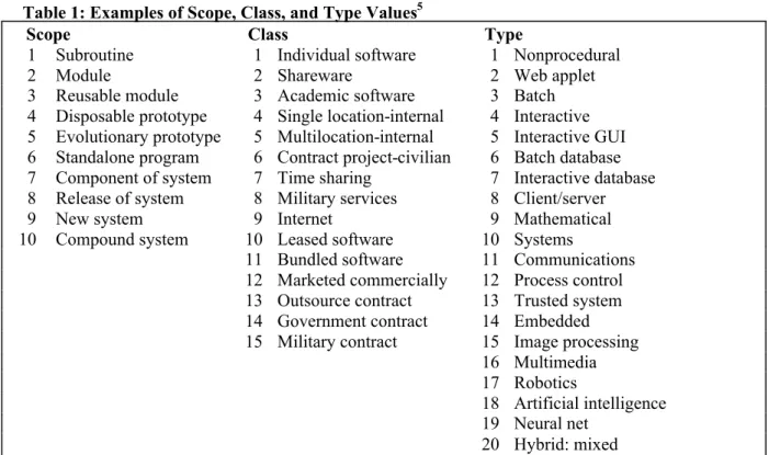
For calculating the estimated function points three kinds of factors have to be defined: the scope, the class and the type. Every factor has a list of values, in which the appropriate value has to be chosen.

Larger numbers have more significance than smaller numbers.

Table 1: Examples of Scope, Class, and Type Values⁵

Scope Class Type

1 Subroutine 1 Individual software 1 Nonprocedural

2 Module 2 Shareware 2 Web applet

3 Reusable module 3 Academic software 3 Batch 4 Disposable prototype 4 Single location-internal 4 Interactive 5 Evolutionary prototype 5 Multilocation-internal 5 Interactive GUI 6 Standalone program 6 Contract project-civilian 6 Batch database 7 Component of system 7 Time sharing 7 Interactive database 8 Release of system 8 Military services 8 Client/server

9 New system 9 Internet 9 Mathematical

10 Compound system 10 Leased software 10 Systems

11 Bundled software 11 Communications 12 Marketed commercially 12 Process control 13 Outsource contract 13 Trusted system 14 Government contract 14 Embedded 15 Military contract 15 Image processing

16 Multimedia 17 Robotics

18 Artificial intelligence 19 Neural net

20 Hybrid: mixed

For utilizing this rough sizing method, it is only necessary to follow the three steps⁶:

1. Apply the numeric list values to the project to be sized in terms of the scope, class, and type factors (see Table 1).

2. Sum the numeric values from the three lists.

3. Raise the total to the 2.35 power.

5 [Jones98], p185

6 [Jones98], p185/186

Applying this method to the following two examples⁷: Client/server application:

Step 1

Scope = 6 (standalone program) Class = 4 (internal-single site) Type = 8 (client/server)

Step 2 Sum = 18

Step 3 18^2.35 = 891

891 function points is a rough approximation, but it is not too bad because client/server applications are often in the range of 1000 function points.

Personal application:

Step 1

Scope = 4 (disposable prototype) Class = 1 (individual program) Type = 1 (nonprocedural)

Step 2 Sum = 6

Step 3 6^2.35 = 67

Most personal applications are less than 100 function points, so this approximation is a good approximation.

Even if these results yield good approximations, it is not recommended to use this method for any other purpose than estimating size prior to the requirements definition. Nevertheless, this method can be very useful for estimating the range of costs.

The ranking of this calculating method is not fix. Users can both experiment with their own ranking system and vary the power used for the function point approximation.

2.2.2 Estimation Methods derived from Function Points

A lot of different metrics can be derived from the function point metrics. In his book Estimating Software Costs⁸ T.C. Jones describes 12 rules of how to estimate other metrics based on function points. On the next pages I will describe these rules.

Rule 1 – Sizing source code volumes

Because a lot of software projects have been measured with lines of code (LOC) and function points, empirical ratios have been developed for converting LOC in function points, and vice versa. These rules are based on the number of logical statements rather than physical ones because physical LOC are more sensitive to the programming style and the language.

Rule 1:

One function point = 320 statements for basic assembly language One function point = 213 statements for macro assembly language One function point = 128 statements for the C programming language One function point = 107 statements for the COBOL language

One function point = 107 statements for the FORTRAN language One function point = 80 statements for the PL/1 language

7 [Jones98], p185/186

8 [Jones98], Chapter 11

One function point = 71 statements for the ADA 83 language One function point = 53 statements for the C++ language One function point = 15 statements for the Smalltalk language

As we can see from the table, the conversation factor of a procedural source code is about 100-to-1.

An object-oriented programming language results about 20 statements per function point on average.

This rule of thumb has a high margin of error because programming style and programming language can vary the results significantly! The direct conversation from the number of lines to function points is called backfiring.

Rule 2 – Sizing Software Plans, Specifications, and Manuals

Software development is very paper intensive. Especially for large systems, producing paper documents costs much more than the coding. Here is a remarkable example: “For a few really large systems in the 100’000-function point range, the specifications can actually exceed the lifetime reading speed of a single person, and could not be finished even by reading 8 hours a day for an entire career!”⁹

Rule 2:

Function points raised to the 1.15 power predict approximate page counts for paper documents associated with software projects.

Rule 2 predicts the approximate volume of the documentation. This calculation refers to a normal page used in the United Stated with about 400 English words on it. The power of the calculation can drift depending on the kind of standard used for the documentation (e.g. ISO 9000-9004).

Rule 3 – Sizing Creeping User Requirements

New or changing requirements after the completion of the requirements analysis are a serious problem of software development. These additional expenses can be calculated with another rule of thumb:

Rule 3:

Creeping user requirements will grow at an average rate of 2 percent per month from the design through coding phases.

According to practical value experience, the range of creeping requirements goes from close to 0 to 5 percent per month. A better requirements analysis can reduce the cost of creeping requirements! In order to avoid disagreements on creeping requirements, it is important to specify the cost for creeping requirements in the contract. A time-dependent calculation has advantages because the later the changes the bigger the costs.

Rule 4 – Sizing Test-Case Volumes

The function point metric can also be useful for calculating the number of test cases.

Rule 4:

Function points raised to the 1.2 power predict the approximate number of test cases created.

There are a lot of different kinds of test cases, such as unit testing, system testing, etc. This rule of thumb should be used with caution because it shows only the sum of all test cases!

9 [Jones98], p192

Rule 5 – Sizing Software Defect Potentials

The defect potential is the sum of all errors in a software development project. There are five major kinds of errors¹⁰:

1. Requirements errors 2. Design errors 3. Coding errors

4. User documentation errors

5. Bad fixes, or secondary errors introduced in the act of fixing a prior error

More than half of all software defects are found in the first two points. To know the defect potential is important for the overall cost estimation, so a rule of thumb can be very useful.

Rule 5:

Function points raised to the 1.25 power predict the approximate defect potential for new software projects.

A similar rule can also predict the defect potential for enhancement. Because of possible defects in the base system (latent defects), the number of function points has to be raised with the 1.27 power.

Rule 6 – Sizing Testing Defect-Removal Efficiency

After having estimated the software defects it is also useful to know an approximation for the defect- removal efficiency. There are some rules as well:

Rule 6:

Each software test step will find and remove 30 percent of the bugs that are present.

The efficiency of testing is extremely low! Less than one bug out of three can be found by testing.

An Example: Let us assume that we want to develop a personal application with about 70 function points (FP). Applying Rule 5 and raising 70 FP to the 1.25 power gives us about 200 bugs and defects.

By applying Rule 6 you will find about 30% percent of the bugs: 60 bugs out of 200. We repeat this testing step (with another function test) and yield 42. Still 98 bugs are left! If you continue testing by using this method you will have to repeat these steps about 8 to 9 times and you will still have about 10 bugs left!

Thus, the tests have to be repeated to get a high quality level. Fortunately, there are also other methods with better efficiency.

Rule 7 – Sizing Formal Inspection Defect Removal Efficiency

In fact, formal design and code inspection have a higher efficiency. To perform a formal inspection, for example a review, is not cheap. Different employees have to participate in the review. They also need some preparation time. Despite this expense, the formal inspections have the best return on investment because testing and maintenance costs can be reduced drastically.

Rule 7:

Each formal design inspection will find and remove 65 percent of the bugs present.

Each formal code inspection will find and remove 60 percent of the bugs present.

10 [Jones98], p196

Rule 8 – Postrelease Defect-Repair Rates

It is also interesting how many bugs a maintenance programmer can repair per staff month.

Rule 8:

Maintenance programmers can repair 8 bugs per staff month.

According to T. C. Jones¹¹ this maintenance repair rate has been around the software industry for more than 30 years and still seems to work. This value can possibly be improved with good defined processes and tools.

2.2.3 Rules of Thumb for Schedules, Resources, and Costs

The next part will focus on the prediction of schedules, resources and costs. There are also some simple rules which can be calculated with a pocket calculator, a spreadsheet or even mentally.

First we have to focus on two key concepts¹²:

1. The assignment scope (A scope) is the amount of work for which one person will be responsible on a software project.

2. The production rate (P rate) is the amount of work that one person can perform in a standard time period, such as a work hour, workweek, work month, or work year.

These two rates can be expressed with convenient metrics such as function points, source code statements or word per page!

Rule 9 – Estimating Software Schedules

The most important topic for clients, project managers and software executives is usually the schedule estimation, which can be approximately calculated with rule 9.

Rule 9:

Function points raised to the 0.4 power predict the approximate development schedule in calendar months.

The power of this formula depends on the kind of project. (A military software usually takes more time than others.)

This rule should not be used for serious business purposes either! This result is just a rough approximation but can be very useful as a sanity check! It has to be compared with historical data within the own company, and the power has to be adapted to the historical values.

11 [Jones98], p199

12 [Jones98], p200

Rule 10 – Estimating Software Development Staffing Levels

For planning a project it is important to know how many personnel will be needed. The next rule can help you to estimate this number.

Rule 10:

Function points divided by 150 predict the approximate number of personnel required for the application.

It is based on the A scope¹³. This means that a technical staff member is responsible for 150 function points. Of course this value depends on the skills and experience of the staff. Nevertheless, it can help as a starting point for a detailed staff analysis.

Rule 11 – Estimating Software Maintenance Staffing Levels

Rule 11 is similar to the preceding rule and can help you to estimate the number of personnel required to maintain a software project.

Rule 11:

Function points divided by 750 predict the approximate number of maintenance personnel required to keep the application updated.

In other words, one person can keep about 750 function points of software operational!

Rule 12 – Estimation Software Effort

Rule 12:

Multiply software development schedules by number of personnel to predict the approximate number of staff months of effort.

An example to explain this rule:

For example Microsoft Word 2000 is about 5000 function points (FP) in size.

• Applying Rule 9 and raising 5000 FP to the 0.4 power yields about 30 calendar months.

• Using Rule 10 and dividing 5000 FP by 150 gives a staff of about 33,3 full-time personnel.

• Multiplying 30 calendar months by 33.3 personnel yields a total of about 999 staff months to build MS Word.

(“Incidentally, another common but rough rule of thumb defines a staff month as consisting of 22 working days with 6 productive hours each day, or 132 work hours per month.”¹⁴)

13 Assignment scope

14 [Jones98], p204

3. Further Manual Software Cost-Estimation Methods

In this chapter I will give a short introduction to some other manual techniques. There is to be found more detailed information in B. Boehm’s book: Software Engineering Economics¹⁵.

3.1 Expert Judgment

In the expert judgment technique, one or more experts hand in an estimation of the costs of a software project. The experts use their experience and their understanding of this project.

There are different advantages and disadvantages :

+ An expert is able to factor in the difference between a past and a future project. He can recognize mistakes and therefore avoid difficulties.

+ He can also factor in exceptional personal characteristics and interactions!

- The estimation depends on the objectivity of the estimator, who may be biased or unfamiliar with the important factors of the project.

In order to reduce the disadvantages, the Delphi techniques have been developed.

3.1.1 The Standard Delphi Technique

In order to solve the problem of the objectivity, more than one expert is involved in the estimation.

The different estimations will be combined to one single estimation.

The Standard Delphi technique has its origin at The Rand Corporation in 1948. It has its name from the location of the ancient Greek oracle.

There are five steps to notice¹⁶:

Standard Delphi Technique for Cost Estimation

1. Coordinator presents each expert with a specification and a form upon which to record estimates.

2. Experts fill out forms anonymously. They may ask questions to the coordinator, but should not discuss the situation with each other.

3. Coordinator prepares a summary of the experts' responses on a form requesting another iteration of the experts' estimate, and the rationale behind the estimate.

4. Experts fill out forms, again anonymously, and the process is iterated for as many rounds as appropriate.

5. No group discussion is to take place during the entire process.

During the entire process, no group discussion is to take place, so nobody can be influenced by others.

15 [Boehm81]

16 [Boehm81], p334

3.1.2 The Wideband Delphi Technique

The written feedback in the standard Delphi technique provides not enough information for the decision-making. So Farquhar and Boehm developed an alternative Delphi technique, the Wideband Delphi technique¹⁷. This technique supports the group discussion.

The Wideband Delphi technique¹⁸: Wideband Delphi Technique

1. Coordinator presents each expert with a specification and an estimation form.

2. Coordinator calls a group meeting in which the experts discuss estimation issues with the coordinator and each other.

3. Experts fill out forms anonymously.

4. Coordinator prepares and distributes a summary of the estimates on an iteration form.

5. Coordinator calls a group meeting, specifically focusing on having the experts discuss points where their estimates varied widely.

6. Experts fill out forms, again anonymously, and Steps 4 to 6 are iterated for as many rounds as appropriate.

This technique is a combination of the standard Delphi technique and the advantages of a group meeting. Anonymity of estimates helps to avoid bias towards more assertive or authoritative members of the group.

3.2 Estimation by Analogy

The cost of a new project is calculated by comparison with the costs of other similar completed projects. For example, we know that a web application developed last year costs about 10’000 CHF.

For the new application we have to program 20% more pages, so we’ll need 2’000 CHF more to cover our costs. On the other hand, our personnel have 10% more experience from the old project, so we subtract 1’000 CHF. As a result, the estimated cost will be around:

10’000 CHF + 2’000 CHF – 1’000 CHF = 11’000 CHF

An advantage of this method is that the estimation is based on experience on completed projects.

Difficulties can be avoided by studying the differences between the new project and the old projects.

On the other hand, this method can be risky because the degree of correlation of the new project with old projects is not so clear.

17 [Boehm81], p335

18 [Boehm81], p335

3.3 Parkinsonian Estimation

Parkinson’s Law [Parkinson, 1957] says: “Work expands to fill the available volume.”

For cost estimation this means that the estimation is equal to the available resource. If a product is finished earlier, the time left will be used to develop less useful things, so the human capital will not be used optimal.

It also can be possible that a project needs more resources than that are available. This estimation is very inaccurate. Thus, it is not recommended for use!

3.4 Price-to-win Estimation

In this method, the estimated costs are dependent on customers budget for a job. So this means that the estimation will be equal to the price for getting a software contract.

We can see the sad result of using this technique in the following quote:

“The price-to-win technique has won a large number of software contracts for a large number of software companies. Almost all of them are out of business today.”¹⁹

Because of underestimation the money went out before the job was done. This is a loose-loose- situation: It is neither for the customers nor for the developers satisfying.

The customer has to accept compromises and the developers have to take care that the project will not become a complete disaster.

Like the Parkinsonian estimation, this technique is not recommended either!

3.5 Top-Down Estimating

The overall cost is estimated by taking all global properties of a project into account. The total cost is then split up among the components. This method can be used in association with the methods above.

The main strength of this technique is that the focus is on system level. The estimation is based on previous experiences, so the important system level functions, such as integration, documentation, etc.

will not be missed. The main weakness is that it is difficult to recognize low-level technical problems.

3.6 Bottom-Up Estimating

In the bottom-up estimation costs are separately estimated by the responsible persons of a component.

The parts are than integrated into an overall estimation.

The advantages and disadvantages are vice versa to the top-down technique. The system level parts are frequently forgotten because of the component focus. So bottom-up estimates are often underestimated. It is important to focus consciously on system level functions therefore.

The bottom-up estimates are more expensive, but they have several advantages. Having each part of the project estimated by the person responsible for its success will be helpful in two ways²⁰:

1. Each estimate will be based on a more detailed understanding of the job to be done.

19 [Boehm81], p337

20 [Boehm81], p338

2. Each estimate will be backed up by the personal commitment of the individual responsible for the job.

Another advantage is that the different estimates have the chance to balance out the overall estimate.

So this result can be very stable!

3.7 Summary

This table shows a summary of the strengths and weaknesses of the discussed software cost-estimation methods²¹:

Method Strengths Weaknesses

Expert judgment • Assessment of representativeness, interactions, exceptional circumstances

• No better than participants

• Biases, incomplete recall

Analogy • Based on representative experience • The degree of correlation of the new project with old projects is not so clear

Parkinson • Correlates with some experience • Reinforces poor practice

Price to win • Often gets the contract • Generally produces large overruns

Top-down • System level focus

• Efficient • Less detailed basis

• Less stable Bottom-up • More detailed basis

• More stable

• Fosters individual commitment

• May overlook system level costs

• Requires more effort

It is often necessary to use a combination of these techniques and to compare the different results!

4. Conclusion

As we have seen, manual techniques and rules of thumb are not very accurate. If precise information about costs of a software project is needed, more accurate methods will be necessary. But if this is not that important and you just need some inaccurate estimations, there are different simple tools. It is very important to question the results of such estimations and to compare it with other values.

5. Bibliography

[Boehm81] Boehm, B. (1981). Software Engineering Economics. Englewood Cliffs, N.J.: Prentice Hall.

[Jones98] Jones, T.C. (1998). Estimating Software Costs. New York : McGraw-Hill.

21 [Boehm81], p342