Steering Zitterbewegung in driven Dirac systems: From persistent modes to echoes

Steering Zitterbewegung in driven Dirac systems: From persistent modes to echoes

Phillipp Reck , Cosimo Gorini , and Klaus Richter

^*

Institut für Theoretische Physik, Universität Regensburg, 93040 Regensburg, Germany

(Received 23 October 2019; revised manuscript received 20 February 2020; accepted 21 February 2020;

published 13 March 2020)

Although Zitterbewegung—the jittery motion of relativistic particles—was known since 1930 and was predicted in solid-state systems long ago, it has been directly measured so far only in so-called quantum simulators, i.e., quantum systems under strong control, such as trapped ions and Bose-Einstein condensates.

A reason for the lack of further experimental evidence is the transient nature of wave-packet Zitterbewegung.

Here, we study how the jittery motion can be manipulated in Dirac systems via time-dependent potentials with the goal of slowing down/preventing its decay or of generating its revival. For the harmonic driving of a mass term, we find persistent Zitterbewegung modes in pristine, i.e., scattering free, systems. Furthermore, an effective time-reversal protocol—the “Dirac quantum time mirror”—is shown to retrieve Zitterbewegung through echoes.

DOI:10.1103/PhysRevB.101.094306

I. INTRODUCTION

Zitterbewegung (ZB), i.e., the trembling motion of rela- tivistic particles described by the Dirac equation, was found by Schrödinger already in 1930 [1,2]. The jittery movement is due to the fact that the velocity operator does not commute with the Hamiltonian, and, therefore, it is not a constant of motion. Indeed, the superposition of particle- and antiparticle- like solutions of the Dirac equation leads to harmonic oscilla- tions with, in the case of electrons and positrons, frequency f

=

2mc

²/

h

∼

10

²⁰

Hz and amplitude given by the Compton wavelength

λC∼

10

⁻¹³

m, whose direct measurement is still beyond experimental capabilities [3].

On the other hand, the requirements for the ZB are not unique to the relativistic Dirac equation but can, in principle, be fulfilled in any two- (or multi-) band system. Examples thereof are solid-state systems with spin-orbit coupling as pro- posed by Schliemann et al. in III–V semiconductor quantum wells [4,5] where the energy spectrum is formally similar to the Dirac Hamiltonian. In a solid-state system, the ZB is directly induced by the periodic underlying lattice [6]. The ZB in systems with low-energy effective Dirac-like dispersion was later proposed for carbon nanotubes [7], graphene [8,9], and topological insulators [10,11]. Recently, the ZB was fur- ther predicted for magnons [12] and exciton-polaritons [13].

ZB signatures can also be found in the presence of magnetic fields, e.g., in graphene [9,14] and III–V semiconductor quan- tum wells with spin-orbit coupling [15].

The first experimental observations of the ZB were achieved with a single

⁴⁰

Ca

⁺

ion in a linear Paul trap [16]

and for Bose-Einstein condensates [17,18] with an induced spin-orbit coupling using atom-light interactions [19].

Recently, indirect experimental realizations of the ZB in solid-state systems were also reported [20,21]. Also motivated

*klaus.richter@physik.uni-regensburg.de

by these, we study time-dependent protocols aimed at pro- longing the ZB duration or at generating revivals by effec- tively time reversing its decay. On the theory side, in one case, graphene in an external monochromatic electromagnetic field was considered, and a multimode ZB, i.e., a ZB with addi- tional emerging frequencies, was obtained but found to decay over time [22]. Another work suggests that time-dependent Rashba spin-orbit coupling in a two-dimensional electron gas might indefinitely sustain the ZB [23], whereas adaptation of the two-photon echo method [24], already employed to detect Bloch oscillations [25–27], was also suggested as a tool to create and measure the ZB in carbon nanotubes [28].

Our goal is twofold: (i) To identify nondecaying ZB modes in driven Dirac systems, e.g., graphene; (ii) to consider the possibility of generating ZB “echoes” exploiting the time- mirror protocols put forward in Refs. [29,30].

We start in Sec.

II

with a succinct introduction to the ZB in a static Dirac system, highlighting the mechanisms leading to ZB decay and laying out our general strategy to counteract it via different drivings. In Sec.

III, we show that a monochro-

matic time modulation of the mass term yields a multimode ZB with more frequencies as compared to driving from a monochromatic electromagnetic field where most importantly additional modes turn out to be long lived. Section

IV

deals with the generation of ZB echoes

/

revivals, which, instead, require a short mass gap pulse. Section

V

concludes.

II. ZITTERBEWEGUNG IN DIRAC SYSTEMS:

FREQUENCY, AMPLITUDES, AND DECAY

Consider the static Dirac Hamiltonian,

H

₀=

hv ¯

Fk·σ+

M

₀σz.

(1) Its eigenenergies are

ε_±

(k)

= ±

M

₀²+

h ¯

²v_F²|k|²= ±M0

1

+κ²,

(2)

where

κ=

hv ¯

F|k|/M0.

(3) The eigenstates are

|ϕk,± =

1

√

2

1

+κ²±√

1

+κ²

1

±√

1

+κ² κ

e

^iγk

|k,

(4) with

γk

being the azimuthal angle of

k

measured from the k

x

axis.

Considering an initial plane wave with wave-vector

k

living in the two bands,

|ψ0,k =

c

⁺_k|ϕk,+ +

c

⁻_k|ϕk,−,

(5) its time evolution is trivially given by

|ψk

(t ) = c

⁺_k

e

^−iωk,+t|ϕk,+ +

c

⁻_k

e

^−iωk,−t|ϕk,−,

(6) with eigenfrequencies ¯ hω

k,±=ε_±

(k). The ZB is generated by the interference term in the time-dependent expectation value of the velocity operator,

v^ZBk

(t )

=

2 Re

c

⁺_k

(c

_k⁻

)

^∗

e

^−istktϕk,−|v|ϕk,+

.

(7) Here,

v= ∇k

H

₀/

h ¯

=v_Fσ

is the velocity operator, and the ZB frequency is given by

h ¯

^stk =ε₊

(k)

−ε₋

(k)

=

2M

0

1

+κ²,

(8) where “st” stands for static. Evaluating the matrix element of the velocity operator for the gapped Dirac system yields both parallel and perpendicular ZBs with amplitudes,

A

^st,_k =vF

2|c

⁺_k||c_k⁻|

√

1

+κ² vF

√

1

+κ²,

(9) A

^st,⊥_k =v_F

2

|

c

⁺_k||

c

⁻_k|v_F.

(10) In the perfect (scattering-free) system described by H

₀

, the ZB of a single

k

mode oscillates without decaying with an amplitude and frequency given by the initial band-structure occupation. On the contrary, the ZB of a wave packet has a transient character [31], i.e., it vanishes over time. For an initial wave packet of the general form

|ψ0 =

d

²

k

ψ0

(k)|ψ

_0,k,

(11) one has

v^ZB

(t )

=

d

²

k

|ψ0

(k )

|²v^ZBk

(t )

,

(12) i.e., the wave-packet ZB is the average of the plane-wave ZB weighted by the

k-space distribution of the initial state. As

different

k

modes have different frequencies, such a collective ZB dephases over time and vanishes. Technically, this is due to the phase e

^−istkt

in Eq. (7), whose oscillations as a function of

k

become faster for increasing time t—and, thus, average progressively to zero. Rusin and Zawadzki give an alternative but equivalent explanation for the ZB decay [32]. They start by considering the movement of the two subwave packets in the different

±

bands, each made up of modes with velocities,

v_±= ∇kε±

(k )

/

h ¯

.

(13) Since

v₊

is antiparallel to

v₋

, the subpackets move away from each other and progressively decrease their mutual overlap,

which translates to a decrease in the interference and, thus, in the ZB [33].

Note that the general velocity of Eq. (13) leads also to other unintuitive effects in solids, e.g., Bloch oscillations. There, a constant electric field leads to oscillations of electrons. The reason is that due to the electric field, the momentum of the electrons changes linearly. Due to a periodic band structure in momentum space, this change leads to an oscillatory behavior of the electrons. As opposed to the ZB, Bloch oscillations have been detected experimentally [25–27].

This paper is devoted to circumventing or reverting the decay of the ZB via a time modulation of the mass term M

0→

M

0+

M (t ). More precisely, we consider the general time-dependent Hamiltonian,

H

=

hv ¯

Fk·σ+

M

0σz+

M (t )σ

z=

H

0+

H

1

(t ), (14) and study two scenarios. The first one is based on harmonic (monochromatic) driving, to be dealt with in Sec.

III. Here,

we follow the strategy of Ref. [22], determining analytically the emerging frequencies of the driven ZB in our system via the rotating-wave approximation (RWA) and the high-driving frequency (HDF) limit. Our analytics are then compared to numerical simulations based on the “

TIME

-

DEPENDENT QUAN

-

TUM TRANSPORT

” (

TQT

) software package [34], which also allows us to study the multimode ZB in regimes not accessible analytically. By taking a Fourier transform of the numeri- cally obtained time-dependent velocity, we can identify the oscillation frequencies and aim at finding out long-lived or possibly nondecaying modes—i.e., we are after oscillations which survive on a long timescale. To single out the long-time oscillations, we Fourier transform the simulation signal for t

>

t

^∗

, where t

^∗

is the time when the amplitude of the initial transient oscillations has decayed below 5% of its T

=

0 value, see Sec.

III C.

The second scenario, discussed in Sec.

IV, is radically dif-

ferent: Rather than looking for long-lived modes in response to a persistent monochromatic driving, we consider the effects of a sudden (nonadiabatic) on-and-off modulation of the gap.

The idea is to use the quantum time mirror (QTM) protocol of Refs. [29,30] to effectively time reverse the sub-wave- packet dynamics. Once the latter are brought back together, we expect a reconstruction of the interference pattern yielding a ZB.

III. DRIVEN ZITTERBEWEGUNG IN DIRAC SYSTEMS:

EMERGENCE OF PERSISTENT MULTIMODES

We start from Eq. (14) with a harmonically oscillating mass term of the form

M (t )

=

M ˜ cos(ω

D

t ), (15) and study the resulting ZB, i.e., we time evolve a given initial state according to

i h ¯

∂

∂tψ(t

)

=

H (t )ψ(t ), (16)

and calculate the expectation value of the velocity operator.

A. Driven Zitterbewegung: Analytics

In the following analytical section, we adapt a procedure from Ref. [22], and details of the derivation can be found in Ref. [35].

1. RWA

The RWA is well known and often used in quantum optics to simplify the treatment of the interaction between atoms, i.e., few-level systems and a laser field. Although, here, we con- sider two bands, the system is effectively a two-level system for any arbitrary

k

as long as

k

is conserved, i.e., for homoge- neous pulses. The conditions for the applicability of the RWA are as follows: (i) The amplitude of the time-dependent part ˜ M has to be small compared to other internal energy scales of the system; (ii) its frequency is in resonance with one of the level spacings

ωD≈^stk

. In that case, all high-frequency terms in the Hamiltonian average out at physical timescales, and only the resonant terms survive [36]. Calculations are performed for a single

k

mode since the collective wave-packet ZB is given by the weighted superposition from Eq. (12).

The goal is to solve the time-dependent Dirac equation (14), i.e., to find for all

k

the time-dependent occupations of its two nonperturbed bands, given certain initial conditions.

One first looks for a SU(2) (pseudo)spin rotation which diagonalizes the time-dependent part of the Hamiltonian.

Then, according to the RWA, only slow terms are kept, i.e., outright static ones or those whose time dependence is given by e

^{±i(ωD−stk)t}

. Faster terms, in our case, with a time dependence of e

^{±i(ωD+stk)t}

or e

^±iωDt

, average out rapidly and are dropped. The equations then decouple, yielding a homo- geneous second-order differential equation of the harmonic- oscillator type. Its time-dependent wave function is then used to compute the expectation value of the velocity operator

v.

The ZB perpendicular to the propagation direction

k

yields

v_⊥k=v_F

h ¯

√

1

+κ²

M ˜

κ {|

A

₊|²

(

+ωR

) sin[(

ωD+ωR

)t ]

+ |A₋|²

(

−ωR

) sin[(ω

D−ωR

)t]

+

2

ωR

Im(A

^∗₋

A

₊

e

^−iωDt

)

},

(17) where we define two additional characteristic frequencies,

=^stk−ωD,

(18)

ωR = ²+

M ˜

²

¯ h

²

κ²

1

+κ².

(19)

The quantities A

_±

are given by the initial conditions (occupa- tion of the two bands) as shown in Appendix

A.

The perpendicular ZB oscillates with three distinct fre- quencies:

ωD, ωD±ωR

. This is in contrast to the standard electromagnetic driving scenario where only the two frequen- cies

ωD±ωR

are obtained [22]. Crucially, the additional

ωD

mode turns out to be nondecaying and, thus, determining the ZB long-time behavior as discussed in Sec.

III C. Although

not shown here, the static limit can be derived from Eq. (17), e.g., by taking the limit ˜ M

→

0.

Similar features arise for the parallel-to-k ZB component,

vk =

hv ¯

F

M ˜

κ{|A₊|²

(

+ωR

) cos[(ω

D+ωR

)t ]

+ |A₋|²

(

−ωR

) cos[(ω

D−ωR

)t]

+

2 Re(A

^∗₊

A

₋

e

^iωDt

)}

+

4v

F

cos(ω

R

t )Re{A

^∗₊

A

₋} +

const. (20) There are now four different frequencies,

ωD, ωD±ωR

, and

ωR

as opposed to the single

ωR

mode of electromagnetic driving [37]. The

ωD

mode is once again responsible for the long-time behavior.

2. HDF

We now investigate the ZB for HDFs ¯ h

ωD

M, thus, ˜ extending the analytically accessible regions. The derivation is similar to the RWA with a different initial SU(2) transfor- mation [22]. The HDF approximation e

^{±2i( ˜M/¯hωD) sin(ωDt)}≈

1 allows for solving the remaining differential equations analyt- ically. One obtains (for the perpendicular ZB)

v_⊥k= −

1 k

const

+

2

^stk

Im

B

₊

B

^∗₋

e

^istkt

−

4 ˜ M k hω ¯

D

M

0

¯

h sin(

ωD

t )Re

B

₊

B

^∗₋

e

^istkt ,

(21) and (for the parallel ZB)

vk = −

1 k

const

+

4 M

₀

¯ h Re

B

₊

B

₋^∗

e

^istkt +

2 ˜ M

k h ¯

ωD

^stk

sin(ω

D

t )Im

B

₊

B

₋^∗

e

^istkt ,

(22) where the quantities B

_±

are again given by the initial condi- tions, see Appendix

A. Bothv_⊥k

and

vk

have an

^st_k

mode as in the static case as well as weaker O( ˜ M

/

h ¯

ωD

) oscillations at

ωD±^stk

. Their suppression, going along with the survival of the

^stk

mode, has a simple physical reason: Electrons cannot respond to a driving much faster than the frequencies of their intrinsic dynamics and, therefore, oscillate at

^st_k

as if no extra field was present.

B. Driven Zitterbewegung: Numerics

We test our RWA and HDF analytical results against nu- merical simulations based on the

TQT

wave-packet propaga- tion package [34], which uses the Lanczos method [38] to evaluate the action of the time-evolution operator on a wave packet to time evolve an initial state numerically.

In the following, the initial state is a Gaussian wave packet:

ψ0

(k)

=

1

√π

k

²

exp

−

(k

−k0

)

²

2

k²

,

(23)

that equally occupies both bands and which is time evolved

in the presence of the time-dependent mass potential. If not

otherwise specified, we take M

₀

as the energy unit, choose

the center wave-vector

k₀

such that ¯ hv

F

k

₀ =

0

.

4M

₀

, and a

k-

space width of

k= |k0|/10, where

k

0= |k0|. The velocity

expectation value is obtained by numerically computing the

ωR ωD+ω^R ωD−ωR 2ωD+ωR

2ω_D−ω_R

ω/M0

0 2 4 6

ωD/M0

(b)

ω^D ω^R ω^D

+ω^R

|ωD−ωR|

M/M˜ 0

0 1 2 3 4 5 6 0 1 2 3 4 5

ω/ωD

(c) (a)

0 10 20tωD/(2π)30 40

-2 -1.5

-1 -0.5

0 0.5

1

v(t)/vF

0 1 2 ω/ωD3 4

32 34

0 2 4 6

|v(ω)|2(a.u.) ωR

0 1 2 3

|v(ω)|2 (a.u.) 0 1 HDF

RWA RWA

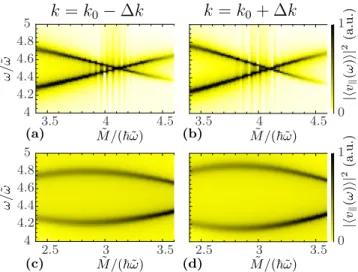
FIG. 1. Frequencies of a driven ZB. (a) The parallel ZBv(t)is shown both as a function of time (black) and as its Fourier transform (blue), i.e., as function of ω for ωD=2M0/h¯ and ˜M=1.2M0. The inset shows a closeup for longer times. Peaks appear in the Fourier transform at multiple integers of ωD with satellite peaks at a distance ofωR (orange line at the first peak) away from the major peaks. (b) and (c) Fourier transform ofvas a function of driving frequencyωD (for fixed ˜M=0.5M0) and amplitude ˜M(for fixedωD=2M0/¯h) of the time-dependent mass term, respectively.

The blue vertical line in (c) marks the function shown in panel (a) (indicated by the blue arrow). The expected frequencies from the RWAωD, ωD±ωR, andωR are shown (red, solid line) as well as higher-order terms inωD (red, dashed line). For smaller ˜M, up to M˜ ≈1.3M0, the RWA results Eq. (20) are well recovered whereas for larger ˜M, the RWA is not justified anymore. In all plots, we choosek0 such thatε₊(k0)=0.4M0, and, thus, the ZB frequency corresponding to the staticH0is^stk₀≈2.15M0/h.¯

time derivative of the wave-packet position expectation value,

v(ti

) =

r(ti+1

) − r(t

i

)

δt ,

(24)

at each time t

i

with

δ

t as the simulation time step. The static ZB frequency is

^stk₀ ≈

2.15M

0/

h. ¯

The upper trace in Fig.

1(a)

shows the simulation data for

v

as a function of time (black) for large-amplitude driving ˜ M

=

1.2M

0

at frequency

ωD=

2M

0/¯

h. After an initial irregular transient (t

ωD/

2

π

20), a stable periodic signal settles. Note, however, that the long-time response is not monochromatic as manifest from the zoom-in inset. We dis- cuss this in detail below in Sec.

III C.

The numerically computed fast Fourier transform of

v

(t ) is shown in Fig.

1(a)

(blue). Clear peaks are visible at integer multiples

ω=

n

ωD,

n

∈N

accompanied by smaller satellite peaks at nω

D±ωR

. To visualize the dependence on the different parameters, the fast Fourier transform

|v

(ω)|

²

is shown in density plots, each vertical slice corresponding to one simulation at a given value of the driving frequency

ωD

for a fixed amplitude ˜ M

=

0

.

5M

₀

[panel (b)] and at a given value of the driving amplitude ˜ M for a fixed frequency

ωD=

2M

0/

h ¯ [panel (c)]. The vertical blue line in panel (c)

ω/M0

0 5

ωD/M0

0 1 2 3 4 5

v(ω)2(a.u.) ωD/M0

0 1 2 3 4 5

long t modes

(a) (b)

M˜ = 1.2M0

M˜ = 1.2M0

0 1

all modes

ω/M0

0 2 4 6 8 10

M/M˜ 0

0 1 2 3 4 5

v⊥(ω)2 (a.u.) 0 1

M/M˜ 0

0 1 2 3 4 5

(c) (d)

ωD= 2M0 ωD= 2M0

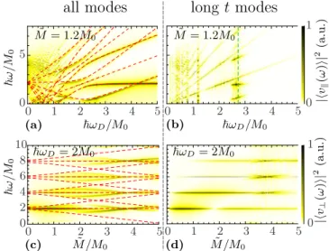
FIG. 2. Searching for infinitely long surviving modes of the Zit- terbewegung. The left panels (a) and (c) show plots of all appearing ZB modes whereas the right panels (b) and (d) show the modes which survive a long time (as defined in the text). The modes of the perpendicular and parallel ZBsv_⊥(ω)(upper panels) andv(ω) (lower panels) are shown as a function either of the parameterωD

or of ˜M. Analytically expected modes from the RWA (red, dashed lines) are indicated in the left panels. In general, the surviving modes for long times are the ones not depending onk, e.g., multiples ofωD, or weaklykdependent where∂ωR/∂k=0 [indicated by the green dashed lines in (b)].

corresponds to the simulation shown in panel (a) as indicated by the blue arrow. The ZB behaves as expected from the HDF Eq. (22) for large

ωD

(only mode:

^stk₀

). Furthermore, in the region of validity of the RWA, the frequencies

ωD, ωD±ωR

, and

ωR

are present [solid red lines in panels (b) and (c)] as long as ˜ M M

0

and

ωD≈^stk₀

. Note that, for ¯ hω

D

M, ˜ one has

ωR −−−−→ωD→∞ ωD−^stk₀

so that one of the RWA modes becomes

|ωD−ωR|−−−−→^{ωD→∞ st}k0

and coincides with the HDF result. Indeed, the line labeled

|ωD−ωR|

in panel (b) merges with the RWA modes in the region

ωD≈^stk₀

.

In addition to the expected frequencies, further modes also emerge, obtained by adding integer multiples of

ωD

to the lower ones. The reason for the appearance of the latter is given in Appendix

B, based on higher-order time-dependent

perturbation theory.

C. Long-time behavior of the Zitterbewegung

We now search for long-lived ZB modes. If present, they should easier to be detected experimentally. The long-time ZB frequencies are easily obtained from the simulation data: By considering the Fourier transform of the signal starting at a time t

>

t

^∗

after the initial transient has decayed. The time t

^∗

is defined by the condition that the relative ZB amplitude in the time-independent setup has decreased to less than 5% in both

v

and

v_⊥

(if both are present).

In Fig.

2, the ZB frequency spectra for a Fourier transform

starting at t

=

0 (left panels) and for a Fourier transform

starting at t

^∗

(right panels) are compared for several parameter

combinations. The simulation data are the same on both sides,

only the time interval for the fast Fourier transform changes:

[0, t

max

] to identify all modes or [t

^∗,

t

max

] to single out the long-lived ones, where t

_max

is maximal time of the simulation.

Comparing the left and right panels in Fig.

2, it is clear

that some branches fade out completely, some remain nearly unchanged, and others still survive only in a small parameter regime. This can be understood by recalling the general arguments from Sec.

II

where the ZB decay was shown to be due to dephasing caused by the varying ZB frequencies of different

k

modes building the propagating wave packet.

Therefore, the ZB modes that weakly depend on

k—or are

outright

k

independent—will not dephase and should, thus, survive.

The RWA and HDF approximations indicate that the only

k-independent ZB mode has frequency ωD

. Indeed, in all plots, modes with frequencies

ωD

and integer multiples thereof are unchanged in the long-time limit. The strangely regular shape of the time line for the long-lived ZB in the closeup of Fig.

1(a)

might be explained by the fact that mostly integer multiples of

ωD

survive. This corresponds to a discrete Fourier transform and, thus, to a

ωD

-periodic behavior in time. These

k-independent modes are the only truly infinitely

lived ones. However, they might be expected since it is not too surprising that a system driven at

ωD

will respond at the same frequency (and at multiples thereof). More interestingly, Fig.

2

(b) shows that sections of certain branches survive even at frequencies which are not integer multiples of

ωD

. Such modes are locally

k

independent, i.e., the ZB frequencies are stationary with respect to changes in

k. Using Eq. (19) for the

RWA frequency

ωR

and setting

∂ωR/∂k=^!

0 yields

∂^stk

∂

k

+vF

M ˜

²

¯ h

κ

(1

+κ²

)

² =

0

⇔ −M0ωD+^stk

M

0+

M ˜

²

2

√

1

+κ²³ =

0. (25) To analyze the data in Fig.

2(b)

where the ZB is shown as a function of

ωD

, we solve Eq. (25) for

ωD

,

ω^critD =^stk

1

+

M ˜

²

4M

₀²

1 (1

+κ²

)

²

.

(26) The result is shown as a green dashed line in Fig.

2(b),

confirming that the system also responds (persistently) at frequencies not directly related to that of the driving. Different ZB modes depend on

k

via

ωR

, and, indeed, each branch intersecting the green line has long-lived components around the intersection point. The long-lived modes are huddled around the exact value of

ω^critD

2.75M

0/¯

h (for the given simulation parameters). Note that additional surviving modes, i.e., (locally)

k

independent, appear at low frequencies, e.g.,

ωD=

1.2M

0/

h. The latter cannot be explained within the ¯ RWA, which loses validity for

ωD< ^stk =

2

.

15M

₀/

h. ¯

The last kind of modes which survive for longer times can be seen in panels (c) and (d) at ˜ M

≈

4M

0

where the nω

D

modes are crossed by other modes. However, their frequencies are close to the surviving nω

D

modes, and, therefore, they do not, particularly, alter the long-time behavior, which is why we relocate the numerical discussion of their appearance to Appendix

C.

IV. ZITTERBEWEGUNG ECHOES VIA EFFECTIVE TIME REVERSAL

We now discuss an alternative way to retrieve late-time information of the ZB. Instead of Eq. (15), we consider a short mass pulse of the form

M (t )

=

M, ˜ t

0<

t

<

t

0+t,

0, otherwise. (27)

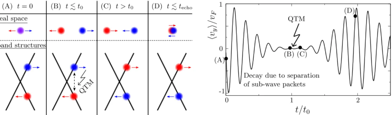
The steplike form (27) is chosen for definiteness and mathe- matical convenience only. Indeed, as long as the mass pulse is diabatically switched on and off, it can act as a QTM, i.e., it can effectively time reverse the dynamics of a wave packet, irrespective of its detailed time profile [30,39]. In general, we expect that effective time reversal will yield an echo of the initial ZB. This is apparent when recalling that a propagating two-band wave packet progressively splits into two subwave packets, each composed of states belonging to one of the two bands, and that the ZB is due to the interference between the subwave packets. As the spatial overlap between the latter decreases, so does their interference, causing the ZB to decay [32]. A properly tuned mass pulse, however, causes the subwave packets to invert their occupation of the two bands (the former electronlike state becomes a holelike state and vice versa) and, hence, inverts their direction of motion.

Thus, the subwave packets start to reapproach each other, and, as they recover their initial overlap, the interference pattern yielding a ZB is reconstructed, see Fig.

3.

A. ZB echoes: Analytics

We closely follow Refs. [29,30] and quantify the strength of the ZB echo by considering the density correlator,

C

(t )

=

d

²

r

|ψ

(r

,

t )

||ψ

(r

,

0)

|,

(28) i.e., the spatial overlap between the initial density and the one at time t. This measure is appropriate for wave packets which are initially well localized in space. The mass pulse action on an initial eigenstate is

k

conserving (the pulse is homogeneous in space) and can, in general, be expressed as a change in the initial band occupation,

|ψk,s =

B

s

(k, t )|ϕ

k,s +

A

s

(k, t )|ϕ

k,−s.

(29) For gapped Dirac systems, the transition amplitude A

s

is independent of s

,

A

s→

A. One has [30]

A(k, t )

=

iκ M ˜

M

₀²+

M

²κ²√

1

+κ²

sin Mt

¯ h

1

+κ²

,

(30) with M

=

M

₀+

M ˜ and

κ

from Eq. (3). Each

k

mode con- tributes to the echo only with its component which switches bands (reverses the velocity) during the mass pulse, i.e., the term proportional to A in Eq. (29). Moreover, the components proportional to B

s

are irrelevant and will be neglected in the following. Given a general initial wave packet,

|ψ0 =

k

ψ0

(k)

ψ₀^k

=

k

ψ0

(k)(c

⁺_k|ϕk,+ +

c

⁻_k|ϕk,−),

(31)

QTM

(A) t= 0 (B) tt0 (C) t > t0 (D) ttecho

t/t

0

v

y

/v

F band structures

real space QTM

(A) (B) (C)

(D)

0

-1 1

0 1 2

Decay due to separation of sub-wave packets

FIG. 3. Retrieving decaying Zitterbewegung through a spin-echo-type time-reversal mechanism. Left panel: An initial wave packet with components in both bands separates due to the different band velocities∝∇kε(k). The decreasing overlap between the subwave packets causes the ZB to decay [(A) to (B)], see the time line of the velocity expectation valuevyin the right panel. Via a short QTM pulse att₀, the subwave packets switch bands, thus, reversing their velocities and returning to their initial positions [see (C)]. The recovery of the overlap in (D) leads to a ZB revival. The black dots in the right panel belong to the time instants sketched in the left panel.

with

|

c

⁺_k|²+ |

c

⁻_k|² =

1, and this amounts to considering only its effectively time-reversed part,

|ψecho

(t

)

=

k

ψ0

(k)

ψecho^k

(t

)

=

k

ψ0

(k )

s=±1

c

^s_k

e

^−iωk,st0

×

A(k, t )e

^{−iωk,−st1}|ϕk,−s.

(32) Here, ¯ hω

k,±s=ε_±

(k), see Eq. (2), whereas t

=

t

0+t+

t

1

is a generic time after the pulse. For the initial wave packet (31), the ZB at time t

reads

v^ZB(t

)

=

d

²

k|ψ

0

(k)|

²v^ZBk

(t

). (33) Before the pulse, each

k-mode contribution is [see Eq. (7)]

v_i^ZB

k

(t

<

t

0

)

=

2 Re

c

⁺_k

(c

⁻_k

)

^∗

e

^−istktϕk,−|vi|ϕk,+

,

(34) where i

∈ {x,

y} denotes the direction.

Recall that the wave-packet ZB decay is due to dephasing among its constituent modes: At longer times t , the expo- nential e

^−istkt

oscillates faster as a function of

k

and, thus, averages out in the integral (33). To reverse this dephasing process, the phase of the oscillations must be inverted. For a time t

after the pulse, the velocity expectation value of each

k

mode of the effectively time-inverted wave-packet

|ψecho

in Eq. (32) yields

v_i^ZB

k

(t

)

= |A(k)|²

2 Re

c

⁺_k

(c

_k⁻

)

^∗

e

^{−istk(t0−t1)}ϕk,+|vi|ϕk,−

.

(35) Indeed, the kinetic phase of the complex exponential e

^{−istk(t0−t1)}

decreases with t

₁

(the time elapsed after the pulse) and reaches zero at t

1=

t

0

—i.e., the initial phase is recovered.

The recovery happens simultaneously for all

k

modes, leading to complete rephasing at the echo time t

echo=

2t

0+t

[40].

For a wave packet centered at

k₀

and narrow enough to approximate A(k)

≈

A(k

₀

), the transition amplitude can be taken out of the integral (see Ref. [29]), and the ratio of the revived ZB amplitude in direction i, B

_i^revival

to the initial one

B

_i^initial

is

B

^revival_i

B

^initial_i ≈ |

A(k

₀

)

|²,

(36) with i

∈ {

x

,

y

}

. On the other hand, the correlator, Eq. (28), is approximately given by the transition amplitude [29],

C(techo

)

≈ |A(k0, t

)|, (37) so that we expect

B

^revival_i

B

^initial_i ≈C²

(t

echo

) (38)

to be checked below numerically.

As a side remark, note that the ZB echo bears a certain resemblance to the spin echo: The latter is achieved when dephased oscillating spins—i.e., an ensemble of two-level systems—are made to rephase again by a

π

pulse. Here, an analogous rephasing among oscillating

k

modes—i.e., an ensemble of delocalized states with a given dispersion—is obtained via the QTM protocol.

B. ZB echoes: Numerics

We numerically compute the correlator

C(t

), Eq. (28) via

TQT

for gapless (M

0=

0) and gapped (M

0 =

0) Dirac systems. In both cases, the transition amplitude is given by Eq. (30). The initial wave packet is composed of

k

modes from both branches of the Dirac spectrum, which is necessary for the ZB at t

=

0. As a proof of principle, we use a Gaussian wave packet, narrow in reciprocal space (k

=

k

0/8), and

compare the results with the estimates Eqs. (36)–(38). The wave packet is peaked around

k₀=

(k

₀,

k

₀

)

^T/√

2 with

κ0=

¯

hv

F

k

₀/

M

=

0

.

4.

Figure

4(a)

compares the correlator

C(t

) to the relative am-

plitude of the revived ZB. The velocities are normalized with

respect to the initial ZB amplitude B

_i^initial

. As expected from

the analytics, at the echo time t

_echo

2t

₀

, the ZB amplitude

coincides with the echo strength

C²

(t

_echo

)

|

A(k

₀,

t )

|²

.

Panel (b) shows the relative amplitude both in the x and

the y directions, Eq. (36), and echo strengths

C²

(t

echo

) as

-0.5 0 0.5

1

vx(t)/Bx^initial

vy(t)/By^initial

C²(t)

0 0.5 1 1.5 2 2.5

t/t0 00 5 10Δt M/15 20 25

0.2 0.4 0.6 0.8 1

0.1 0.2 0.3

(a) κ0

0.2 0.4 0.6 0.8 1

B^revivalx /B^initialx

B^revivaly /B^initialy

C²(techo) (b) (c)

M0= 0 M0= 0 M0= 0

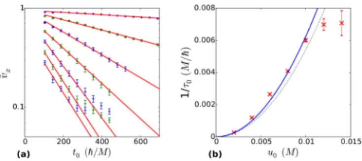
FIG. 4. Comparison between ZB echo simulations and analytical estimates for a gapless [panels (a), (b)] and a gapped [panel (c)] Dirac system. In panel (a), both the velocity expectation value and the correlationC²(t), Eq. (28), are shown as functions of time, whereC²(t) and the ZB amplitude coincide attecho2t0, in agreement with Eq. (38). Panel (b) compares the echo strengthC(techo)≈ |A(k0, t)|(see Ref. [29]), to the relative amplitude of the revived ZB both in thex- and they-directions as a function oftfor fixedκ0=hv¯ _Fk₀/M=0.4. The expected agreement can be seen. Panel (c) shows analogous data for a gapped Dirac system, wheret=1.4 ¯h/Mwhereas the mean wave vector of the wave packet, i.e.,κ0, is varied.

functions of

t, i.e., of the pulse duration t

. Numerically, the amplitude of the echo is obtained by searching for the largest difference between consecutive local maxima and minima, which are in a certain time interval around the ex- pected echo time t

_echo=

2t

₀+

t

,

I

=

[t

_echo−τ,

t

_echo+τ

], to exclude the initial ZB from the automatic search in the data.

We define the echo amplitude B

^revival_i

of the ZB as B

^revival_i =

max

t∈I

v^max_i

(t )

−v^min_i

t

+π/^ZBk₀

2

,

(39)

where

v_i^max

is a local maximum and

v^min_i

is a local minimum of the velocity in direction i. Here, we use as interval width

τ =

0.5t

0

, but the exact value does not matter as long as the revival is included in the interval I and the ZB that does not belong to the revival is excluded. Since no difference between

C²

and the ratio between initial and revived amplitudes is visible in panel (b), the echo of the ZB has the expected strength, see Eq. (38).

In panel (c), a gapped Dirac system (M

0=

0) is considered, and the echo strengths are shown for varying mean wave- vectors

κ0=

hv ¯

F

k

₀/

M and fixed

t

=

1

.

4 ¯ h

/

M. The relative amplitude of the revived ZB matches the quantum time mirror echo strength obtained by the correlation

C²

(t

echo

), confirming again our analytical expectations.

Hence, we have shown that the ZB echo behaves as the quantum time mirror in Ref. [30] where, for different band structures, the effects of position-dependent potentials in the Hamiltonian, such as disorder and electromagnetic fields are discussed additionally. To show that we recover the same results for the ZB echo also in these cases, we discuss the effect of disorder on the ZB echo in Appendix

E. As expected,

the relative echo strength decreases exponentially in time where the decay time is given by the elastic-scattering time.

Although we stay on the single-particle level, Rusin and Zawadzki [28] suggest that methods from nonlinear laser spectroscopy, such as the established two-photon echo [24]

can be used to extract the ZB in a many-particle setup as has been performed for Bloch oscillations [25–27]. Most impor- tantly, these suggested methods together with our proposed

ways to prolongate the lifetime of the ZB, could be sensitive enough to finally measure the ZB in solids.

V. SUMMARY AND CONCLUSIONS

The ZB as a promient hallmark of dynamics governed by the Dirac equation has so far resisted a direct measurement, although it is expected to exist in solid-state physics in sys- tems, such as graphene, that can be described by an effec- tive Dirac equation. We theoretically investigated different aspects of the dynamics of the driven ZB via analytical and numerical methods within a single-particle picture [41]. The basic concepts for understanding and describing the ZB in static Dirac systems were introduced in Sec.

II

where we also outlined our two strategies to counteract the ZB decay (that has hindered direct measurements) witj both strategies based on the time-dependent Hamiltonian (14).

The first one was discussed in Sec.

III. A periodically

driven mass term in (gapped) Dirac systems, see Eq. (15), was shown to give rise to a multimode ZB. The latter long- time behavior reveals the existence of persistent ZB modes, emerging at frequencies stationary with respect to wave- vector changes and not necessarily at simple multiples of the driving frequency. Such long-lived modes should allow for an experimental detection of the ZB much easier than standard rapidly decaying ZB modes.

The second strategy was dealt with in Sec.

IV. The ZB

revivals or echoes were shown to be generated via a protocol acting as a quantum time mirror [29,30], i.e., requiring a short pulse opening temporarily a mass gap as defined in Eq. (27).

The echo signal decays exponentially for weak disorder, i.e., behaves as expected in the presence of impurities or imper- fections. Although ZB experiments remain challenging [20], it would be interesting to transfer established spin-echo-based protocols—mostly T

2

-weighted imaging—to the ZB.

ACKNOWLEDGMENTS

We acknowledge support from Deutsche Forschungsge-

meinschaft (DFG, German Research Foundation) through