Testing linear forms of variance components by generalized fixed-level tests

Testing linear forms of variance components by generalized xed{level tests

Boris Weimann ¹ Department of Statistics

University of Dortmund Vogelpothsweg 87 D{44221 Dortmund

Germany

Abstract

This report extends the technique of testing single variance components with gen- eralized xed{level tests | in situations when nuisance parameters make exact testing impossible | to the more general way of testing hypotheses on linear forms of vari- ance components. An extension of the denition of a generalized test variable leads to a generalized xed{level test for arbitrary linear hypotheses on variance components in balanced mixed linear models of the ANOVA{type. For point null hypotheses an alternative for the known method is given, which ist straightforward in contrast to the classic form. An example (2{way nested classication with random eects) illustrates the way how to use the results and simulation studies are carried out to prove the quality of the presented methods.

Key Words: Variance components, generalized xed{level test, mixed linear models, nui- sance parameters, linear hypotheses, approximate testing.

1 Introduction

For various statistical models there do not exist exact tests for the hypotheses of interest because of nuisance parameters. Such situations can always occur if the model includes two or more random eects. Typical representatives of this class of models are the mixed linear models.

Literature is widely available for approximative and asymptotic tests for many very special situations. A classical example is the approximative test by Satterthwaite (1946), an F{test with adapted degrees of freedom for hypotheses on single variance components. In a paper

1

This research was supported by the Deutsche Forschungsgesellschaft (DFG); Sonderforschungsbereich

475

1

by Thursby (1989), a number of approximative tests is compared. All of these procedures are only of restricted usability.

The concept of testing with generalized p{values was introduced by Tsui and Weerahandi (1989). Weerahandi (1991) and Zhou and Mathew (1994) used generalized p{values for tests on variance components in their papers, where the hypotheses were usually only formulated for single variance components.

In this paper the test with generalized p{values is extended to the case of arbitrary linear hypotheses in balanced mixed linear models. In order to do this, the denition of a gen- eralized test variable which was rst introduced by Tsui and Weerahandi (1989) has to be extended, because it proves to be too restrictive. The new procedure is demonstrated on the example of the hierarchical two{way classication. Simulation studies show that the new method usually holds the nominal signicance level quite well, even in the case of small data sets.

Two{sided hypotheses which are to be tested against composite alternatives are a problem mostly unregarded up to now. Weerahandi (1995) proposed a solution, but he did not formulate a concrete construction principle for the test procedure. This paper will show up a straightforward procedure which, as far as the signicance level is concerned, is comparable to tests for one{sided hypotheses.

In variance component models the problem of a quite small power may occur for some parts of the alternative for any kind of test. For some constellations of parameters the empirical power functions are given for a special testing problem in the above mentioned hierarchical two{way classication. A detailed analysis of the power function will be a subject of further research.

The restriction to balanced models can be abandoned in some situations. Khuri (1990) showed that generalized p{values can be applied if the model in unbalanced on the last stage only. An application of this procedure to testing linear hypotheses and a generalization to arbitrary forms of unbalancedness is desirable.

2 General testing principle

Consider an observable random vector Y with the cumulative distribution function F(y;), where = (#;^T)^T is a vector of unknown parameters, # being the parameter of interest, and a vector of nuisance parameters. Let be the sample space of possible values of Y and be the parameter space of #. An observation of Y is denoted by y.

2

Denition 2.1

A random variable of the form T = T(Y;y;) is said to be a generalized test variable if it has the following three properties:

1. tobs =T(y;y;) does not depend on unknown parameters.

2. When#is specied,T has a probability distribution that is free of nuisance parameters.

3. For xed y and , Pr(T t^j#) is a monotone function in# for any given t.

Without loss of generality the rst property can be considered to be redundant, because if it is not satised we can cross over to the transformation ~T := T(Y;y;)^;T(y;y;) and impose properties 2 and 3 on ~T.

Property 2 is imposed to ensure that p{values based on generalized test variables are com- putable when # is specied. Property 3 ensures that the sample space can be stochastically ordered on the basis of the generalized test variable. If Pr(T > t) is a nondecreasing function in #, then T is said to be stochastically increasing in#.

Consider the problem of testing one{sided hypotheses of the form H⁰ : # #⁰ vs. H¹ : # > #⁰ ;

(1)

where #⁰ is a prespecied value of the parameter #.

Denition 2.2

LetT =T(Y;y;) be a stochastically increasing (in the parameter of interest#) test variable according to denition 2.1. Then, the subset of the sample space dened by

Cy() = ^fY ^2jT(Y;y;)tobs^g

(2)

is said to be a generalized extreme region for testing H⁰ against H¹.

Denition 2.3

If Cy() is a generalized extreme region according to (2), then p(tobs) = sup

##⁰Pr(Y ²Cy()^j#) (3)

is said to be its generalized p{value for testing H⁰. 3

Corollary 2.4

The generalized p{value according to (3) is equivalent to p(tobs) = Pr(Y ²Cy()^j#=#⁰) ;

(4)

which is easy to determine.

Proof:

This follows directly from property 3 of a generalized test variable: if T is stochastically increasing in #, the supremum over ⁰ =^f#^j# #^0g is obtained on the upper boundary of

⁰. ²

Denition 2.5

Letp(tobs) be a generalized p{value on a continuous generalized test variableT =T(Y;y;).

Let H⁰ : # ^{2 0} be the null hypothesis being tested against the alternative H¹ : # ^{2 1}. Then, the rule dened as

reject H⁰ if p(tobs) (5)

is said to be a generalized xed{level test of level .

Corollary 2.6

The generalized p{value according to (3) as a function of the observed value tobs resp. y is not uniformly distributed over the interval [0;1]. For that reason, the generalized xed{level test according to (5) is not an exact test of level , but an approximate one.

Proof:

Assume a continuous generalized test variableT. The generalized p{value p(tobs) = Pr(T(Y;y;)tobs^j#=#⁰) = 1^;FT(tobs;#⁰)

is a function of the observed value of T. Considering the observed tobs = T(y;y;) as a random variable T = T(Y;Y;) leads in general to dierent distributions for T and T, because only the distribution of T depends on the observed value tobs. From the probability integral transform it follows, that FT(T) has a uniform distribution over the interval [0;1].

Because of

p(T) = Pr(T(Y;y;)T(Y;Y;)^j#=#⁰)

= 1^;FT(T;#⁰)

6 1^;FT(T)

it follows, that p(T) in general does not have an uniform distribution over [0;1]. ² 4

Denition 2.7

Let (y;#) := Pr(Y ² Cy()^j#) be the data{based power function of T. A test based on a generalized extreme region Cy() is said to be p{unbiased if

(y;#)(y;#⁰) for all #²¹ ; (6)

and p{similar (on the boundary) if, given any y ², (y;#⁰) =p(tobs)

(7)

does not depend on the nuisance parameters , where p(tobs) ist the generalized p{value according to (3).

This concept of testing with generalized p{values was rst introduced by Tsui and Weera- handi (1989) and is presented in detail in Weerahandi (1995).

3 Testing point null hypotheses

Consider point null hypotheses and composite alternative hypotheses of the form H⁰ : # =#⁰ vs. H¹ : #⁶=#⁰

(8)

where #⁰ is a particular value of the parameter that has been specied.

In such situations Weerahandi extends denition 2.1 by substituting

4. Given any xed tobs and , the probability Pr(T ²Cy()) is a nondecreasing function of (i)#^;#⁰ when ##⁰, and (ii) #^0;# when # < #⁰.

for property 3 of a generalized test variable.

By this denition the data{based power function(y;#) increases on ¹ with the distance to ⁰. Particularly the resulting generalized xed{level test is p{unbiased. A problem occurs when the generalized extreme region is to be constructed, because the construction is not as obvious and clearly determined as in the case of one{sided null hypotheses.

A possibility to avoid the problem of constructing a generalized extreme region is to use the same generalized test variable for one{sided and point null hypotheses and dene the generalized p{value for the point null hypothesis in the usual way by

p(tobs) = 2min^fPr(T(Y;y;)> tobs);Pr(T(Y;y;)< tobs)^g (9) = 2min^fPr(Y ²Cy());1^;Pr(Y ²Cy())^g

5

This proceeding also guarantees the p{unbiasedness of the resulting generalized xed{level test. Moreover, there cannot be problem{immanent reasons against the incidentally assumed symmetry of the generalized extreme region. Nevertheless by using (9) for point null hy- potheses it is no longer possible to construct extreme regions of maximal length or other optimality properties.

4 Linear hypotheses

Consider testing problems on linear hypotheses of the form H^0I : d^T =c vs. H^1I : d^{T 6}=c ;

H^0II : d^T c vs. H^1II : d^T > c ; H^0III : d^T c vs. H^1III : d^T < c ; (10)

where d²IRⁿ,c²IR and n is the dimension of the parameter space .

In the case of testing linear hypotheses, the classication of the parameter vector into the parameter of interest # and the vector of nuisance parameters has to be modied.

In general, all parameters now are of interest, but all parameters also function as nuisance parameters.

So we transform the hypotheses (10), leaving an arbitrary single parameter on the left side of the special null hypothesis:

H^0I : i = 1di

0

@c^;X

j⁶⁼idjj

1

A vs. H^1I : i ⁶= 1di

0

@c^;X

j⁶⁼idjj

1

A ; H^0II : i 1

di

0

@c^;X

j⁶⁼idjj

1

A vs. H^1II : i > d¹i

0

@c^;X

j⁶⁼idjj

1

A ; H^0III : i 1

di

0

@c^;X

j⁶⁼idjj

1

A vs. H^1III : i < d¹i

0

@c^;X

j⁶⁼idjj

1

A ; (11)

Now by denition i takes the role of the parameter of interest (#) and all otherj (j ⁶=i), collected in the vector

:= (¹;:::;i^;1;i⁺¹;:::;n)^T ; function as nuisance parameters.

It will be necessary to modify the denition of a generalized test variable, because property 2 in the case of testing linear hypotheses will prove to be too restrictive. So we come to an adjustment of denition 2.1:

6

Denition 4.1

A random variable of the form T = T(Y;y;) is said to be a generalized test variable if it has the following three properties:

1. tobs =T(y;y;) does not depend on unknown parameters.

2. Wheni is specied, and under the assumption of H^0I (according to (11)), the random variable T has a probability distribution that is independent of the vector of nuisance parameters .

3. For xed y and , Pr(T t^ji) is a monotonic function of i for any given t.

The other denitions in section 2, related to the new denition of a generalized test variable, are no further aected and can be kept in the original form.

Without loss of generality let a generalized test variable be dened as stochastically in- creasing rather than stochastically monotonic in the parameter of interest. In the case of a stochastically decreasing random variable T it is either possible to invert the inequalities in (12) or, for example, to cross over to the transformation T := 1=T which then once again is stochastically increasing in the parameter of interest.

So, the generalized p{values for the three testing problems (10) resp. (11) are given for H^0I : p(tobs) = 2minPr(T(Y;y;)tobs^jH^0I) ; Pr(T(Y;y;)tobs^jH^0I) H^0II : p(tobs) = Pr(T(Y;y;)tobs^jd^T=c)

H^0III : p(tobs) = Pr(T(Y;y;)tobs^jd^T=c): (12)

Calculating p(tobs) under the assumption d^T = c is equivalent to determining the special supremum over H⁰. Because of the monotonic property of T, the supremum in all cases is placed on the boundary.

7

5 Mixed linear models

Consider mixed linear models of the form z X!;^Xm

i⁼¹_i²Ui

!

; i.e. E(z) =X! ; Cov (z) =^Xm

i⁼¹²_iUi ; (13)

with

X!=^Xq

i⁼¹Xi!i = 1n+^Xq

i⁼²Xi!i and Um =In :

If we cross over to a reduced model that is invariant with respect to mean value transforma- tions, we get

y = ProjR⁽X^)?z =Mz with M =In^;XX⁺ ;

whereR(X) is the range of the matrixX and X⁺ is the Moore{Penrose inverse ofX. So,y is the projection of z onto the complement of R(X) and it follows that

y 0;^Xm

i⁼¹_i²Vi

!

with Vi =MUiM : (14)

In ANOVA{models V¹;:::;Vm are linearly independent and there always exists a basis of pairwise orthogonal projectors P¹;:::;Pm which span the same vector space asV¹;:::;Vm. So, the basis transformation matrix = ('ij)i;j⁼¹;::::m is determined by

Vi = ^Xm

i⁼¹'ijPj ; i= 1;:::;m : (15)

The sum of squares Si and mean squares Mi are given by Si = z^TPiz ; i= 1;:::;m ;

Mi = 1trPiz^TPiz ; i= 1;:::;m : (16)

Under the assumption of normality of the random vectorz is follows, that the mean squares Mi are stochastically independent with expectation

E(Mi) = ^Xm

⁼¹²'i ; i= 1;:::;m ; (17)

8

and the following terms have central ²{distributions:

trPi Mi

E(Mi) ^2tr_Pⁱ : (18)

For some special null hypotheses | if two mean squares have the same expectation under H⁰| (18) can be used to construct exact F{tests. In general a construction of exact F{tests is impossible.

For more detailed information about balanced mixed linear models see Hartung et al. (1997) or Khuri and Sinha (1998) for the unbalanced case.

For the problem of testing an arbitrary linear hypothesis of variance components (cf. (11)) consider the following random variable

T(Y;y;²) =

X

l²Ll E(Ml)sl

Sl +⁰c ⁰AsSⁱi + ^X

k²Kk E(Mk)sk

Sk

; (19)

with ² = (²¹;:::;_m²)^T, si the observed value of Si, K;L ^f1;:::;i^;1;i+ 1;:::;m^g, constants k;l ²IR and

A = E(Mi)^;_i²'ii+'ii

2

41 di

0

@c^;X

j⁶⁼idj²_j

1

A 3

5 ; (20)

so that

⁰A+ ^X

k²Kk E(Mk) = ^X

l²Ll E(Ml) +⁰c ; (21)

and all added terms shall be nonnegative:

kE(Mk) 0 ⁸ k ²K ; ⁰A0 ; lE(Ml) 0 ⁸ l ²L ; ⁰c0 : (22)

9

Theorem 5.1

The random variable T(Y;y;²) from (19) with assumptions (21) and (22) possesses the three properties of a generalized test variable according to denition 4.1.

Proof:

1. The observed value of T tobs = T(y;y;²) ⁽¹⁹⁾=

X

l²Ll E(Ml) +⁰c ⁰A+ ^X

k²Kk E(Mk)

(21)= 1

is constant and therefore especially independent of any parameters.

2. Since k;l and si are constant and due to (18)

X

k²Kk E(Mk)sk

Sk and ^X

l²Ll E(Ml)sl

Sl

are linear combinations of independent 1=²{expressions, free of any unknown para- meter. ⁰ and care constant. Finally, for the left term in the denominator ofT in (19) we get

⁰AsSⁱi = ⁰si A

E(Mi) E(Mi) Si

H=^{I0 0}si E(Mi) Si ; (23)

also a 1=²{expression, which at least under the assumption of H^0I is free of nuisance parameters.

3. By construction the parameter of interest _i² (the former i in section 4) in T only appears in E(Mi) in the denominator of (23), which again only appears in the de- nominator of T in (19). With respect to the vector of variance components ² we have

T(Y;y;²) ^/ q¹ q² A

E(Mi) +q³ :

Because of (22) it follows that q¹;q²;q^{3 2} IR⁺⁰, and for that reason T is stochastically increasing in_i².

With 1., 2. and 3. T indeed is a generalized test variable in the sense of denition 4.1. ² The question that occurs is how to get the constants k and l. This can be done by an iterative proceeding:

10

Construction principlefor generating generalized test variables for testing linear hypothe- ses in balanced mixed linear models.

1. Formulate and transform the linear hypothesis of interest, so that a single parameter _i² is isolated on one side of the hypothesis as it is done in (11).

2. For generating T iteratively start with the expression ⁰=A which yields all variance components except for_i² and A is given by (20).

3. The aim now is to set tobs equal to 1. Therefore we have to add 1=²{expressions in the numerator and denominator of T.

4. To nd an admissible set of k and l, the easiest way is to eliminate the variance components according to their appearance in the model (14) from left to right. For example: If the leftmost variance component in the numerator (that is not yet egalized in the denominator) is to be egalized, take that 1=²{expression according to (18) with an expectation (17) whose leftmost variance component is the one to be egalized.

5. The last step is to set ⁰ which is clearly determined as ⁰ :=⁰'ii=di by the former proceeding.

6 An illustrative example

The balanced 2{way nested classication model with random eects is given by yijk = +ai+bij+eijk i= 1;:::;r j = 1;:::;s k= 1;:::;t

with E[yijk] = ; ai (0;_a²) ; bij (0;_b²); eijk (0;_e²) (24) ai;bij and eijk stochastically independent :

Under the assumption of normally distributed random eects ai, bij and eijk, we have the following distribution statements for the sums of squares (cf. (18)):

Sa (st_a²+t_b²+_e²)²_r^;1 Sb (t_b²+_e²)²_r⁽_s^;1) Se _e²²_rs⁽_t^;1) :

11

A generalized test variable for arbitrary linear hypotheses (under the restriction of d^{1 6}= 0) is

T(Y;y;²) = 1^; sd² d¹

!

(t_b²+²_e)sb

Sb +sd² d¹ _e²se

Se + st d¹c

std¹¹⁽c^;d²b^2;d³e²) +t²b +e²

sa

Sa +std³ d^{1 2}ese

Se

(25)

= 1^;sd²

d¹

! sb

²_r⁽_s^{;1) +}sd² d¹ se

²_rs⁽_t^{;1) +} st d¹c

std¹¹⁽c^;d²_b^2;d³_e²) +t²_b +_e² st_a²+t_b²+_e² sa

²r^;1 + std³ d¹ se

²_rs⁽_t^;1)

H=^I0 1^; sd² d¹

! sb

²_r⁽_s^{;1) +} sd² d¹ se

²_rs⁽_t^{;1) +} st d¹c sa

²_r^{;1 +}std³ d¹ se

²_rs⁽_t^;1)

Because no assumptions aboutd²IR³except ford^{1 6}= 0 have been made, negative terms can occur in T. Should this be the case, these negative terms have to be added to the numerator and the denominator of T, which neither inuencestobs = 1 nor leads to a dependence of the generalized test variable on nuisance parameters.

Suppose the hypotheses of interest are for example H^0I :²_a=_b² vs. H^1I :_a^{2 6}=_b²

(26) and

H^0II :_a^{2 2}_b vs. H^1II :_a² > _b² : (27)

This means d= (1;^;1;0)^T and c= 0, and the generalized test variable T is T(Y;y;²) = (1 +s) sb

²_r⁽_s^{;1) ;}s s²_rs^(e_t^;1) st_b²+t²_b +_e²

st_a²+t²_b +_e² sa

²_r^;1 :

Since it is not obvious whether T is a monotone function in _a², the function T(Y;y;²) = (1 +s) sb

²_r⁽_s^;1) st_b²+t_b²+_e²

st_a²+t_b²+_e² sa

²_r^{;1 +}s s²_rs^(e_t^;1) 12

is regarded and then T obviously is a stochastically increasing function in_a². This necessary transformation is not a consequence of the general construction principle (cf. section 5), but caused by using (25) with an arbitrary d ² IR³. In the case of starting with a certain hypothesis and a xed d²IR³ the problem of negative term in T does not occur.

Provided H^0I is true, then T(Y;y;²) = (1 +s) sb

²_r⁽_s^;1) sa

²_r^{;1 +}s s²_rs^(e_t^;1) :

The generalized xed{level test is given by the rule Reject H^0I

H^0II at the nominal level ; if

(2min^fPr(T >1);Pr(T < 1)^g Pr(T >1)

)

< : The probabilities P(T > 1) andP(T <1) are determined by simulation.

For various constellations of the parameters r;s;tand ²_a=_b², with_e² = 1 and the nominal signicance level of = 0:05 the following generalized p{values resulted from simulation studies (1000 runs in each simulation):

p(tobs) p(tobs) r s t ²_a=_b² H^0I H^0II r s t _a² =_b² H^0I H^0II 3 4 2 0:2 0:040 0:059 6 2 2 0:2 0:040 0:058 3 4 2 1 0:055 0:056 6 2 2 1 0:044 0:052 3 4 2 5 0:062 0:054 6 2 2 5 0:050 0:053 3 4 2 10 0:061 0:052 6 2 2 10 0:050 0:053 3 4 8 0:2 0:041 0:068 2 5 3 0:2 0:036 0:067 3 4 8 1 0:042 0:057 2 5 3 1 0:038 0:053 3 4 8 5 0:043 0:054 2 5 3 5 0:046 0:044 3 4 8 10 0:042 0:054 2 5 3 10 0:047 0:044

The simulations show, that even with small sample sizes the approximative tests have an es- timated signicance level near to the nominal one. With risingrthe approximation becomes even better. In general the one{sided test for problem (27) tends to be more conservative than the two{sided test (26).

13

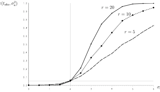
For s = 3, t = 2, b = 2, e = 1 and a nominal signicance level of = 0:05 the following data{based power{functions (tobs;a²) are computed by simulation in dependence on r:

r= 20

r = 10

r = 5

Figure 1: Estimated power of the two{sided test (cf. 26) as a function of a

a

(tobs;²_a)

r = 20

r = 10 r= 5

Figure 2: Estimated power of the one{sided test (cf. 27) as a function ofa

a

(tobs;²_a)

14

For the estimated data{based power{functions (tobs;_b²) in dependency of _b², with a = 2 and under the same parameter constellation we get the following result:

r = 20 r= 10

r= 5

Figure 3: Estimated power of the two{sided test (cf. 26) as a function ofb

b

(tobs;²_a)

r= 20 r= 10

r = 5

Figure 4: Estimated power of the one{sided test (cf. 27) as a function of b

b

(tobs;²_b)

15

References

Hartung, J., Elpelt, B., and Voet, B. (1997). Modellkatalog Varianzanalyse. R. Oldenbourg, Muenchen.

Khuri, A. I. and Sinha, B. K. (1998). Statistical Tests for Mixed Linear Models. John Wiley

& Sons, New York.

Khuri, I. A. (1990). Exact tests for random models with unequal cell frequencies in the last stage. Journal of Statistical Planning and Inference,24^{, 177{193.}

Satterthwaite, F. E. (1946). An approximative distribution of estimates of variance compo- nents. Biomet. Bulletin,2^{, 110{114.}

Thursby, J. G. (1989). A comparison of several exact and approximative tests for structural shift under heteroscedascity. Journal of Econometrics, 53^{, 363{386.}

Tsui, K. and Weerahandi, S. (1989). Generalized p{values in signicance testing of hypothe- ses in the presence of nuisance parameters. Journal of the American Statistical Association,

84^{, 602{607.}

Weerahandi, S. (1991). Testing variance components in mixed models with generalized p- values. Journal of the American Statistical Association,86^{, 151{153.}

Weerahandi, S. (1995). Exact Statistical Methods for Data Analysis. Springer, New York.

Zhou, L. and Mathew, T. (1994). Some tests for variance components using generalized p{values. Technometrics,36^{, 394{402.}

16