Zooplankton mortality effects on the plankton community of the northern Humboldt Current System: sensitivity of a regional biogeochemical model

(1)

https://doi.org/10.5194/bg-18-2891-2021

Zooplankton mortality effects on the plankton community of the northern Humboldt Current System: sensitivity of a regional biogeochemical model

Mariana Hill Cruz¹, Iris Kriest¹, Yonss Saranga José¹, Rainer Kiko², Helena Hauss^1,3, and Andreas Oschlies^1,3

1GEOMAR Helmholtz Centre for Ocean Research Kiel, Düsternbrooker Weg 20, 24105 Kiel, Germany

2Laboratoire d’Océanographie de Villefranche-sur-Mer, Sorbonne Université, Villefranche-sur-Mer, France

3Kiel University, 24098 Kiel, Germany

Correspondence:Mariana Hill Cruz (mhill-cruz@geomar.de) and Iris Kriest (ikriest@geomar.de) Received: 11 November 2020 – Discussion started: 9 December 2020

Revised: 16 March 2021 – Accepted: 22 March 2021 – Published: 12 May 2021

Abstract.Small pelagic fish off the coast of Peru in the eastern tropical South Pacific (ETSP) support around 10 % of global fish catches. Their stocks fluctuate interannually due to environmental variability which can be exacerbated by fishing pressure. Because these fish are planktivorous, any change in fish abundance may directly affect the plankton and the biogeochemical system.

To investigate the potential effects of variability in small pelagic fish populations on lower trophic levels, we used a coupled physical–biogeochemical model to build scenarios for the ETSP and compare these against an already-published reference simulation. The scenarios mimic changes in fish predation by either increasing or decreasing mortality of the model’s large and small zooplankton compartments.

The results revealed that large zooplankton was the main driver of the response of the community. Its concentration increased under low mortality conditions, and its prey, small zooplankton and large phytoplankton, decreased. The response was opposite, but weaker, in the high mortality scenarios. This asymmetric behaviour can be explained by the different ecological roles of large, omnivorous zooplankton and small zooplankton, which in the model is strictly her- bivorous. The response of small zooplankton depended on the antagonistic effects of mortality changes as well as on the grazing pressure by large zooplankton. The results of this study provide a first insight into how the plankton ecosystem might respond if variations in fish populations were modelled explicitly.

1 Introduction

Eastern boundary upwelling systems (EBUSs) are among the most productive regions in the ocean. Despite their small size, they support a large fraction of the world’s fisheries (Chavez and Messié, 2009). The northern Humboldt Cur- rent System (NHCS) in the eastern tropical South Pacific (ETSP) Ocean is the most productive EBUS, producing 10 % of global fish catches (Chavez et al., 2008) and supporting the fishery of the Peruvian anchovyEngraulis ringens, which is the biggest single-species fishery on the planet (Chavez et al., 2003). The ETSP is also characterised by substantial interannual variability (i.e. El Niño–Southern Oscillation; Holbrook et al., 2012) and an intense midwater oxygen minimum zone (OMZ), resulting in high denitrification rates (Farías et al., 2009).

As in other EBUSs, small pelagic fish are highly abundant (Cury et al., 2000) in the NHCS, building up large populations that are severely affected by climate fluctuations. For example, anchovy biomass in the NHCS fluctuated between 10×10⁶ and 16×10⁶t in the 1960s (Alheit and Niquen, 2004). Its area of distribution spans from northern Peru to northern Chile and the Talcahuano region off central Chile (Fig. 1 in Alheit and Niquen, 2004). During the El Niño event of 1972, it dropped to 6×10⁶t (Alheit and Niquen, 2004), presumably caused by warming and the resulting decrease in upwelling and production. These unfavourable growth conditions for anchovy might have been exacerbated by fishing pressure (Beddington and May, 1977; Hsieh et al., 2006).

From 1992 to 2008, the population of anchovy off the Peru-

(2)

vian coast fluctuated between 3×10⁶and 12×10⁶t (Fig. 13 in Oliveros-Ramos et al., 2017).

The Peruvian anchovy is a planktivorous fish whose diet changes over its ontogenic development. Anchovy first- feeding larvae consume mainly phytoplankton, and when they reach a length of 4 mm their diet gradually switches to zooplankton, especially nauplii of copepods (Muck et al., 1989). Adult anchovies’ main sources of energy are euphausiids and copepods although phytoplankton is still found in their diet (Espinoza and Bertrand, 2008). The other promi- nent small planktivorous fish species in the NHCS is the Pa- cific sardineSardinops sagax, which feeds on smaller parti- cles than anchovy, including phytoplankton and small zooplankton (Ayón et al., 2008a). These two species can therefore be expected to impose a direct top-down control on plankton; at the same time, they may be bottom-up affected by changes in plankton abundance caused by variations in physical forcing.

Pauly et al. (1989) estimated that the total population of anchovy off Peru consumes 12.1 times its own biomass in 1 year. Assuming an area of 6×10¹⁰m²(Ryther, 1969) and a conversion factor of zooplankton wet weight to nitrogen of 1000 mg ww(mmol N)⁻¹(Travers-Trolet et al., 2014a), a fluctuation in anchovy population of 9×10⁶t would result in a change in zooplankton mortality of 5 mmol N m⁻²d⁻¹ from anchovy predation alone, in a top-down-driven ecosystem assuming no non-linearities. The assumption that anchovy can exacerbate a top-down control on zooplankton is supported by a decline in zooplankton concentration in dense aggregations of anchovies (Ayón et al., 2008a, b). On the other hand, co-occurring long-term fluctuations of zooplankton and anchovies at the population scale also indicate a relevant bottom-up control in the NHCS (Alheit and Niquen, 2004; Ayón et al., 2008b).

Numerical models are valuable tools to examine the potential tight coupling across a large range of trophic levels and the mutual interactions among the different components, including top-down and bottom-up effects. Rose et al.

(2010) pointed out the increasing need for so-called end- to-end models of the marine food webs; these set-ups cou- ple models including physical and biogeochemical processes with models for higher trophic levels. When lower-trophic- level (biogeochemical) and higher-trophic-level (fish) models are coupled, the link is typically made at the plankton level, with the former models providing food for the latter (e.g. Travers-Trolet et al., 2014b).

In stand-alone biogeochemical models that do not include higher trophic levels, zooplankton mortality is a closure term, used to return the additional biomass to detritus. It represents all processes that reduce the concentration of zooplankton and are not explicitly included in the model (for instance, predation by gelatinous organisms, predation by higher trophic levels and non-consumptive mortality). For example, Getzlaff and Oschlies (2017) used it to mimic predation and immediate egestion or mortality by higher trophic

levels. Zooplankton mortality may also form the link to fish models, when these are explicitly considered in the context of biogeochemical models (e.g. Travers-Trolet et al., 2014b).

However, there is no consensus on the form of the mortality term, linear (µ·[Z], where[Z]is the zooplankton concentration andµis a mortality rate) and quadratic (µ·[Z]²) being two common forms (e.g. Evans and Parslow, 1985; Fasham et al., 1990; Koné et al., 2005; Kishi et al., 2007; Aumont et al., 2015). A common argument for preferring quadratic to linear mortality is the reduction in unforced short-term oscillations (Steele and Henderson, 1992), although Edwards and Yool (2000) argue that quadratic mortality does not always remove such oscillations. A quadratic mortality term may also be interpreted as an increase in diseases because of high population densities, cannibalism or increased predation due to high densities of prey. Because it is very difficult to determine zooplankton mortality in the field, there is also no agreement on the exact value of mortality (either linear or quadratic), and this term, in practice, is often adjusted to tune the model. However, not using mortality rates based on observations may limit the capability of the model to accurately represent the zooplankton compartment (Daewel et al., 2014) and to draw predictions about the state and dynamics of the marine ecosystem (Anderson et al., 2010). Hirst and Kiørboe (2002) predicted a global mortality of copepods of 0.062 d⁻¹ at 5^◦C and 0.19 d⁻¹at 25^◦C in the field. Two-thirds of such mortality is due to predation. In models, the values of the quadratic mortality rate (hereafter calledµZ) in the literature vary over a large range, from 0.025 (Fennel et al., 2006) up to 0.25(mmol N m⁻³)⁻¹d⁻¹(Lima and Doney, 2004).

For the NHCS, the high variability in forcing, biogeochemistry and plankton and the high abundance of planktivorous fish, together with its economic importance, indicate the need for end-to-end models that include details of all components. However, developing such a model is chal- lenging, and studies in this area have so far focused on either fish (Oliveros-Ramos et al., 2017) or physics and biogeochemistry (Jose et al., 2017). Given the large importance of zooplankton mortality as a link between these two model systems (Mitra et al., 2014) and the uncertainty associated with it, in this study we focus on the effects of this parameter on the biogeochemical system of the ETSP as a first step towards a fully coupled system.

In order to model the highly dynamic nature of both physical and biogeochemical processes in the ETSP, we employed a biogeochemical model specifically designed for EBUSs, coupled to a finely resolved regional circulation model. The coupled model has already been validated against oxygen, nitrate and chlorophyll (Jose et al., 2017); this configuration serves as a starting point and reference for the sensitivity experiments. In this study, we focus on the four plankton groups of the model: small and large phytoplankton and small and large zooplankton. Large phytoplankton is highly abundant near the coast of Peru in the nutrient-rich upwelling region.

Towards the open ocean it is grazed down by its preda-

(3)

tor, large zooplankton; and further offshore, as conditions become oligotrophic, small zooplankton and phytoplankton take over.

In this study, we first extend the model validation by Jose et al. (2017) and assess the reliability of the large zooplankton compartment in the model by comparing it against mesozooplankton observations obtained by net hauls. Note that in this paper we always refer to simulated phyto- and zooplankton by their size class (small or large), while observations are referred to as mesozooplankton. We then present two sensitivity experiments in which we varied the mortality rate of quadratic zooplankton mortality by ±50 %. Model sensitivity is examined with regard to concentrations of model components and inter-compartmental fluxes. Besides the overall response of the prognostic variables to an increase or decrease in zooplankton mortality, we describe how changing zooplankton mortality affects the trophic structure of plankton, with focus on the highly productive coastal domain. Fi- nally we discuss the implications of our study for the plankton community and for modelling higher trophic levels.

2 Methods

2.1 ROMS–BioEBUS model set-up

The Regional Oceanic Modeling System (ROMS; Shchep- etkin and McWilliams, 2005) is a high-resolution, free- surface, terrain-following coordinate ocean model that solves the primitive equations considering Boussinesq and hydro- static assumptions. The Biogeochemical model for Eastern Boundary Upwelling Systems (BioEBUS), which was derived from a N₂P₂Z₂D₂ model from Koné et al. (2005), is coupled online to the physical part (Gutknecht et al., 2013a, b).

In this study the coupled ROMS–BioEBUS model has the same configuration as in Jose et al. (2017). It contains a small, high-resolution domain forced by a larger coarse- resolution domain, using the AGRIF (adaptive grid refine- ment in Fortran) 2-way nesting procedure. The small inner grid has a horizontal resolution of 1/12^◦spanning from about 69 to 102^◦W and from 5^◦N to 31^◦S (Fig. 1). The large outer grid spans from 69 to 120^◦W and from 18^◦N to 40^◦S with a resolution of 1/4^◦. The biological processes occur in three time steps of 900 s for each physical time step of 2700 s in both domains. The two domains have 32 sigma layers with a vertical resolution of less than 5 m at the surface and decreasing to around 500 m at a maximum depth of 4500 m.

The coarse-resolution domain temperature, salinity and horizontal velocity are forced at the lateral boundaries with monthly climatological (1990–2010) SODA reanalysis (Car- ton and Giese, 2008). Both domains are forced at the surface with 1/4^◦ resolution wind velocity fields from QuikSCAT (Liu et al., 1998) and monthly heat and freshwater fluxes from COADS (Worley et al., 2005). At the lateral boundaries

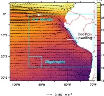
Figure 1.Annually averaged sea surface temperature (^◦C) and horizontal advection vectors (m s⁻¹) and location of the analysed regions (see labels) and of a vertical section for analysing plankton spatial succession (white line at 12^◦S). The coastal upwelling region (see Sect. 2.5) spans from the coast to about 40 to 50 km offshore.

of the coarse-resolution domain, the biogeochemical model is forced with monthly nitrate and oxygen values from CARS (Ridgway et al., 2002) and surface chlorophyll from SeaW- iFs (O’Reilly et al., 1998). Phytoplankton and zooplankton boundary conditions are derived from a vertical extrapola- tion of the chlorophyll data. Detailed information about the boundary and initial conditions and validation of the model is available in Jose et al. (2017).

2.2 Biogeochemical model description

The evolution of a biological tracer in time is represented by Eq. (1). On the right-hand side of the equation, the first term represents the advection with the velocity vectoru. The eddy and molecular diffusion is represented by the second and third terms, whereK_his the horizontal diffusion coefficient andK_zthe vertical diffusion coefficient. The last term is a source-minus-sink (SMS) term due to biological processes.

The full set of equations and detailed explanation about each process are available in Gutknecht et al. (2013a).

∂C_i

∂t = −∇ ·(uC_i)+Kh∇²C_i+∂

∂z

K_z∂C_i

∂z

+SMS(C_i) (1) The BioEBUS model is adapted for the biogeochemical processes specific to the low-oxygen conditions of EBUSs, with some processes being oxygen dependent (see Gutknecht et al., 2013a). It has two compartments of phytoplankton, two compartments of zooplankton and two compartments of

(4)

detritus. The zooplankton and phytoplankton groups are divided into two size classes (small and large). There is not an explicit size parameter in the model; however, the compartments aim at representing the main ecological functions of the plankton community falling within each group. Hence, small phytoplankton (P_S) represents organisms smaller than about 20 µm that require low nutrients such as flagellates, while large phytoplankton (P_L) represents larger organisms such as diatoms. Similarly, small zooplankton (Z_S) simulates the role of a zooplankton community smaller than about 200 µm, such as ciliates, and large zooplankton (Z_L) represents a community larger than 200 µm, such as copepods.

The two size classes of detritus (smallDSand largeDL) are produced from phytoplankton and zooplankton mortality and by release of unassimilated grazing material. The model also contains three compartments of dissolved inorganic nitrogen (NH⁺₄, NO⁻₂ and NO⁻₃), dissolved organic nitrogen (DON), oxygen (O₂) and nitrous oxide (N₂O).

The BioEBUS model (Gutknecht et al., 2013a) includes oxygen-dependent remineralisation processes, which are divided into ammonification, nitrification and denitrification, as well as anammox, and are based on the formulations by Yakushev et al. (2007). N₂O is a diagnostic variable for model output, and its production does not affect the concentration of the other variables. It is based on the parameterisation of Suntharalingam et al. (2000, 2012), which relates the production of N2O to the consumption of O2from decompo- sition of organic matter in oxic and suboxic conditions. O2

concentrations depend on primary production, zooplankton respiration, nitrification and remineralisation. This model includes gas exchange of O2and N2O with the atmosphere.

2.2.1 Phytoplankton

The SMS terms in the small and large phytoplankton compartments are determined by Eqs. (2) and (3), respectively:

SMS(PS)=(1−εP_S)·JP_S(PAR, T ,N)· [PS] (2)

−G^P_Z^S

S· [Z_S] −G^P_Z^S

L· [Z_L] −µ_P_S· [P_S], SMS(PL)=(1−εP_L)·JP_L(PAR, T ,N)· [PL] (3)

−G^P_Z^L

S· [ZS] −G^P_Z^L

L· [ZL] −µP_L· [PL]

−w_P_L· d dz[P_L].

Here G^X_Zⁱ

j represents feeding rates by zooplankton (see Sect. 2.2.2); µ_P_i· [P_i] is the mortality term, representing all not explicitly modelled phytoplankton losses;w_P_L is the sinking speed of large phytoplankton sedimentation, which is an additional loss term for this compartment;ε_P_i is the ex- udation fraction of primary production; andJ_P_i(PAR, T ,N)

is the growth rate limited by light, temperature and nutrients:

JP_i(PAR, T , N )= Jmax_P_i·αP_i·PAR q

Jmax²_P

i+(αP_i·PAR)²

(4)

·f_P_i(NO⁻₃,NO⁻₂,NH⁺₄),

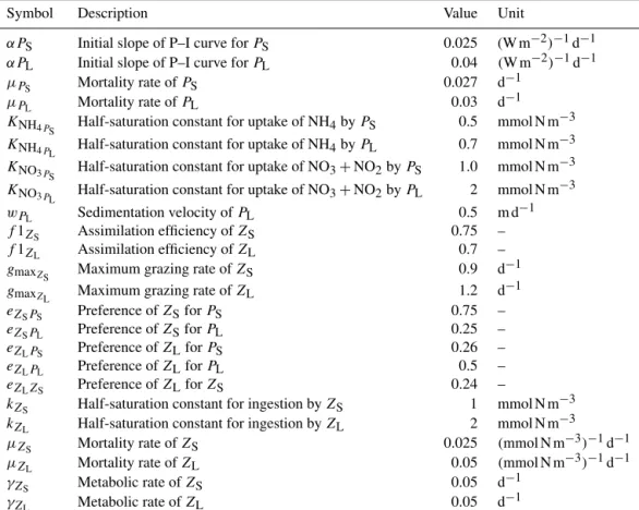
wheref_P_i(NO⁻₃,NO⁻₂,NH⁺₄)is the growth limitation by nutrients, PAR is the photosynthetically available radiation (see Koné et al., 2005), JmaxP_i is the maximal light-saturated growth rate which is a function of temperature andαPi is the initial slope of the photosynthesis–irradiance (P–I) curve (Gutknecht et al., 2013a). Large phytoplankton is characterised by a steeper initial slope of the P–I curve and by larger half-saturation constants for nutrient uptake (see Ta- ble A1). Therefore, it grows better than small phytoplankton under low-light conditions, but its nutrient uptake increases more slowly as nutrient concentrations increase.

2.2.2 Zooplankton

Zooplankton increases its biomass through grazing on phytoplankton and in the case of large zooplankton also on small zooplankton. Metabolism; mortality; and, in the case of small zooplankton, predation by large zooplankton are sink terms.

Predation by fish and other higher trophic levels is implicit in the quadratic mortality term. The biomass lost by metabolism and mortality is assumed to become detritus which may sink to the sediments or become remineralised, and a small fraction of zooplankton losses become ammonium and dissolved organic nitrogen, which is also subjected to remineralisation.

The SMS terms of the small and large zooplankton compartment are determined by Eqs. (5) and (6), respectively:

SMS(ZS)=f1Z_S·(G^P_Z^S

S+G^P_Z^L

S)· [ZS] (5)

−G^Z_Z^S

L· [ZL] −γZ_S· [ZS] −µZ_S· [ZS]², SMS(Z_L)=f1_Z_L·(G^P_Z^S

L+G^P_Z^L

L+G^Z_Z^S

L)· [Z_L] (6)

−γZ_L· [ZL] −µZ_L· [ZL]².

Here f1Z_S and f1Z_L are assimilation coefficients (see also Table A1).G^X_Zⁱ

j is feeding rates of predatorZ_j (either large or small zooplankton) on preyX_i (small and large phytoplankton and small zooplankton) calculated with the formulation by Tian et al. (2000, 2001). There is a linear loss rate accounting for basic metabolism (γ_Z_i) and a quadratic loss rate also referred to as mortality. The mortality parame- tersµ_Z_S andµ_Z_L of the reference simulation are 0.025 and 0.05(mmol N m⁻³)⁻¹d⁻¹ for small and large zooplankton, respectively, as in Jose et al. (2017) and Gutknecht et al.

(2013a).

The feeding rate follows the formulation from Tian et al.

(2000, 2001):

G^X_Zⁱ

j=g_max_Zj·e_Z_j_X_i· [X_i] kZ_j+Ft

, (7)

(5)

wheregmax_Zj is the maximum grazing rate of predatorZj, eZ_jX_i is the preference of predatorZjfor preyXi,kZ_j is the half-saturation constant andFtis the total availability of food for predator Zj. Large zooplankton responds more slowly to changes in food due to the high kZL. In the case of large zooplanktonFt=eZLP_S·[PS]+eZLPL·[PL]+eZLZ_S·[ZS], and in the case of small zooplanktonF_t=e_Z_S_P_S· [P_S] +e_Z_S_P_L· [P_L](Gutknecht et al., 2013a).

2.3 Zooplankton evaluation

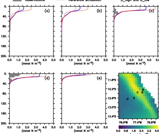
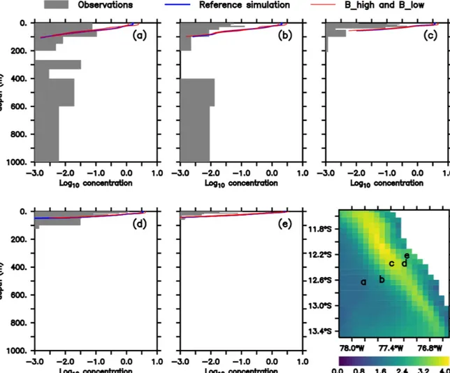
As noted above, this model was already validated against oxygen, nitrate and chlorophyll (Jose et al., 2017). As a com- plement, we here compare the large zooplankton compartment of the model, averaged from January to March, with observational data collected on RVMeteorcruise M93. The samples obtained during this cruise include day- and nighttime hauls with a Hydro-Bios multinet (nine nets, 333 µm mesh) between 10 February and 3 March 2013 on a transect off the Peruvian coast (≈12^◦S; see Fig. 2f), captur- ing the vertical and horizontal gradient in zooplankton concentration. Samples were size-fractionated by sieving and processed according to the ZooScan method (Gorsky et al., 2010). Observations included crustaceans, chaetognaths and annelids greater than 500 µm. For model comparison we con- verted the observation from nighttime hauls to dry biomass according to Lehette and Hernández-León (2009) and further to nitrogen units as suggested by Kiørboe (2013). A detailed description of the zooplankton processing is provided by Kiko and Hauss (2019). Only night observations were compared since our model does not include diel vertical mi- gration.

In both the model and observations, concentration of large zooplankton is greatest in the surface and decreases with depth (Fig. 2). At the surface, modelled concentrations are 1 order of magnitude larger than observations at almost all stations (Fig. 2). Only at station d do observations reach 1 mmol N m⁻³, while the model exhibits maximum values close to 4 mmol N m⁻³. At most stations, the distribution of modelled concentrations is similar to that of observed concentrations in the surface layer (upper 100 m), although model estimates are consistently higher. This is also the case when comparing against a different dataset of observations (see Supplement). Below 100 m, however, model estimates are consistently lower than the observations, which is in particular evident at the deep offshore stations (Appendix B, Fig. B1a and b). Zooplankton in our model does not consume detritus or bacteria; small zooplankton feeds on phytoplankton, and large zooplankton feeds on small zooplankton and on phytoplankton. Therefore, in contrast to observations, its presence is not expected in deep water. In summary, the model matches the observed spatial pattern of zooplankton distribution but tends to overestimate zooplankton concentration in the surface layer and to underestimate it in the

mesopelagic depths. Possible reasons for this mismatch will be discussed in Sect. 4.1.

2.4 Experimental design

To mimic changes in grazing pressure on zooplankton due to small-pelagic-fish biomass fluctuations, we followed the approach by Getzlaff and Oschlies (2017) and varied the mortality rate of each zooplankton compartment by±50 % in comparison to the reference scenario described by Jose et al. (2017). Thereby, an increase in mortality assumes a large consumption of zooplankton by fish, while a decrease in mortality assumes fewer fish. Because the model does not include an explicit compartment for fish, it is assumed that all zooplankton biomass consumed by fish becomes part of the detritus pool via immediate fish mortality and defecation. In reality, a fraction of the biomass is extracted from the system by the fishing industry, predation by sea birds that defecate over land and migrations.

Our model has two zooplankton compartments. In order to explore the different roles of large zooplankton as top predator and small zooplankton as grazer and prey, we performed four experiments, in which we varied the respective mortality rate of large and small zooplankton (0.05 and 0.025 [mmol N m⁻³]⁻¹d⁻¹, respectively) by±50 %:

– A_high with 1.5×µ_Z_L – A_low with 0.5×µ_Z_L

– B_high with 1.5×µ_Z_L and 1.5×µ_Z_S – B_low with 0.5×µ_Z_L and 0.5×µ_Z_S,

where µ_Z_i is the mortality rates of large and small zooplankton. The average nitrogen flux to detritus due to large zooplankton mortality over the upper 100 m depth near the coast of Peru (coastal upwelling region; see Sect. 2.5 and Fig. 1) in the reference scenario is 3.1 mmol N m⁻²d⁻¹(µZ_L· [ZL]², Fig. 3). Neglecting any non-linear and feedback effects within the model, a 50 % change in the mortality rate would result in a change in zooplankton loss due to mortality of 1.55 mmol N m⁻²d⁻¹. It is thus a conservative value, compared to a change of 5 mmol N m⁻²d⁻¹that anchovy population fluctuations could theoretically exert, as estimated in Sect. 1.

All model experiments and the reference scenario were spun up for 30 climatological years. Annual means of the state variables and nitrogen fluxes from the last climatological year of the high-resolution domain were analysed.

2.5 Model analysis

The ETSP is highly dynamic at temporal and spatial scales, with nutrient-rich cold water near the coast of Peru and oligotrophic regions offshore. Therefore, we analysed three different regions: the “full domain” without boundaries (F),

(6)

Figure 2. (a–e)Zooplankton concentrations (mmol N m⁻³). Lines indicate modelled large zooplankton concentrations in the reference scenario and experiments B_high and B_low averaged from January to March. Shaded area shows observed nighttime mesozooplankton biomass concentrations over the sampled depth intervals (m). Observations are lower than 0.1 mmol N m⁻³below 200 m; thus they have not been included. For a plot including deep-water observations, please see Appendix B, Fig. B1, and Fig. 4 in Kiko and Hauss (2019). Bottom right:

modelled large zooplankton biomass concentration at the surface in the reference scenario (mmol N m⁻³) and locations where observations were collected.

Figure 3. Nitrogen flux from large(a) and small (b) zooplankton to detritus due to zooplankton mortality, integrated over the upper 100 m of the water column in the reference scenario (mmol N m⁻²d⁻¹).

an “oligotrophic” region (O) offshore and the “coastal upwelling” region (C) near the Peruvian coast (Fig. 1). Since the upwelling system of Peru is quite heterogeneous with lots of mesoscale processes, we restricted the C region to the very

coastal upwelling area, where the concentration of large phytoplankton is high, up to about 40 to 50 km offshore. Region O was picked to be as far as possible from the nutrient-rich areas along the Equator and along the coast but apart from the domain boundary to avoid boundary effects. For most of our analysis, percentage relative differences between the reference scenario and the other scenarios were calculated.

In addition, we analyse the development of plankton succession from the coast of Peru towards the open ocean at 12^◦S (Fig. 1, white line). Because plankton concentrations are neg- ligible below 100 m depth and we are mainly interested in the plankton community, we focus most of our analysis on the upper water layers. For our analysis we therefore integrate or average plankton concentrations over the upper 100 m or, in the case of shallower waters, down to the seafloor. Also, all analyses in our study take into account only annual averages.

However, we recognise that there is high temporal variability in the NHCS (see Appendix C and Supplement).

(7)

3 Results

We first provide an overview of the general performance of the reference scenario, with respect to the different model components and biogeochemical provinces (Sect. 3.1). We then investigate their response to changes in zooplankton mortality and the response of the plankton ecosystem structure (Sect. 3.2). The coastal upwelling region (C) is especially productive and the habitat of the largest aggregations of small pelagic fish, whose temporal variability inspired this study. Therefore, in Sect. 3.3 we place special emphasis on this region. Finally, we investigate the response of the zooplankton losses due to mortality in the experiments, in order to understand whether the model structure buffers or increases the effect of varying the zooplankton mortality rate on such a term (Sect. 3.4). This would give us an insight into potential feedbacks to higher trophic levels.

3.1 Biogeochemistry and plankton distribution in the reference scenario

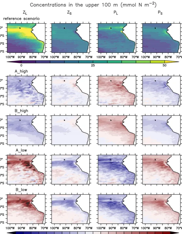
In this section we describe the concentrations of the inorganic and organic compartments in our model reference scenario, averaged between a 0 and 100 m depth (Fig. 4) unless oth- erwise specified. Oxygen concentrations increase offshore, with an average of 226.6 mmol O2m⁻³ in the oligotrophic region (O) compared to 69.7 mmol O2m⁻³ in the coastal upwelling region (Fig. 4). The concentration decreases further below 100 m, reaching an average of 5.3 mmol O2m⁻³ between 100 and 1000 m in the coastal upwelling region (C). Nitrate is the most abundant nutrient all over the domain, ranging from 0.6 in O to 21.7 mmol N m⁻³ in C. On the other hand, ammonium and nitrite are only 0.8 and 3.2 mmol N m⁻³in C, respectively (Fig. 4). Please refer to Jose et al. (2017) for a further in-depth analysis of biogeochemical tracers in the reference scenario.

Phyto- and zooplankton are generally absent in the deep water. In the surface layer between a 0 and 100 m depth (Fig. 4), phytoplankton is clearly favoured by nutrient- rich coastal upwelling, where total phytoplankton reaches 0.93 mmol N m⁻³on average, compared to 0.25 mmol N m⁻³ in the oligotrophic region (Fig. 4). Total detritus follow the concentration trend of plankton, with 0.26 in C and only 0.03 in O.

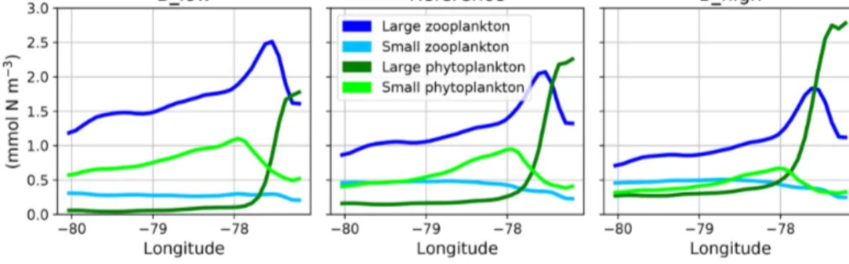
When zooming into the coastal region (Fig. 5), large phytoplankton exhibits a sharp peak near the coast which drops offshore. Moving further offshore, large zooplankton peaks at the decline in the large phytoplankton peak, followed by increased concentrations of small phytoplankton. Given the (Ekman-driven) transport of surface waters (Fig. 1) this spatial pattern might be interpreted as a form of succession as the water is advected offshore. In general, modelled concentrations of large zooplankton are high not only in the coastal upwelling region (Sect. 2.3) but also in large parts of the do-

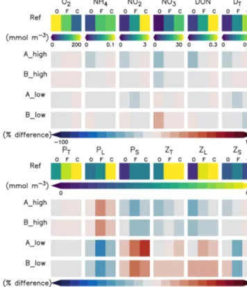
Figure 4.Annually, spatially (oligotrophic (O) region, full domain (F) and coastal upwelling (C) region; see Fig. 1 for further reference) and depth-averaged (0–100 m) concentrations (mmol N m⁻³ or mmol O₂m⁻³) of the biogeochemical prognostic variables in the model reference scenario and normalised percent difference between the reference scenario and experiments.P is phytoplankton;

Zis zooplankton;Dis detritus; DON is dissolved inorganic nitrogen; T is total; L is large; S is small.

main (Fig. 4), except for in the oligotrophic south-western region (Fig. 4).

The growth rate of phytoplankton is limited by temperature, nutrients and light (see Eq. 4). Hence, the spatial pattern of plankton near the coast can be explained by the competitive advantage of large phytoplankton in deep water due to its steeper initial slope of the P–I curve (see Appendix A, Ta- ble A1), eutrophic conditions in the nutrient-rich upwelling water and relatively low predation due to the lack of large zooplankton. This opens a loophole for large phytoplankton to grow in the upwelling waters. As water is transported offshore (Fig. 1), large zooplankton starts to grow and grazes on large phytoplankton. More oligotrophic sunlit conditions even further offshore favour small phytoplankton growth at the surface. Therefore, this first analysis reveals spatial seg- regation and succession from the coast to offshore waters.

These patterns are caused by the model’s parameterisation of plankton groups and their mutual interactions.

(8)

Figure 5.Zonal distribution of surface plankton concentrations at 12^◦S annually averaged in the reference and the two B scenarios, respectively. The location of this section is indicated as a white line in Fig. 1.

3.2 Response to zooplankton mortality

When changing zooplankton mortality, the inorganic variables (Fig. 4) are not noticeably affected by the experiments.

Plankton responds very similarly to changes in mortality in experiments A and B (Fig. 4 and Appendix D, Fig. D1).

Phytoplankton and large zooplankton follow the same direction of response in all regions: concentrations of large zooplankton decrease in the high mortality scenario and increase in the low mortality scenario, as could be expected.

Large phytoplankton responds inversely to large zooplankton, evidencing a top-down control of its main grazer. On the other hand, the response of small phytoplankton is inverse to that of large phytoplankton. In contrast, small zooplankton shows an asymmetric response to changes in mortality, as it mainly decreases in the low mortality scenarios but responds only weakly in the high mortality scenarios (Fig. 4 and Ap- pendix D, Fig. D1).

The spatial plankton distribution along the transect (Fig. 5) remains the same when zooplankton mortality changes, but the absolute concentrations of each compartment change. In all scenarios large phytoplankton peaks close to the coast.

When large zooplankton concentrations are reduced because of its higher mortality in experiment B_high, the large phytoplankton peak increases (Fig. 5, right). Similarly, large phytoplankton decreases with lower zooplankton mortality, due to higher grazing of zooplankton on phytoplankton (Fig. 5, left). This pattern is also similar in experiments A. Because the largest effects occur in the very productive coastal region (C), in the following section we narrow our analysis to this domain.

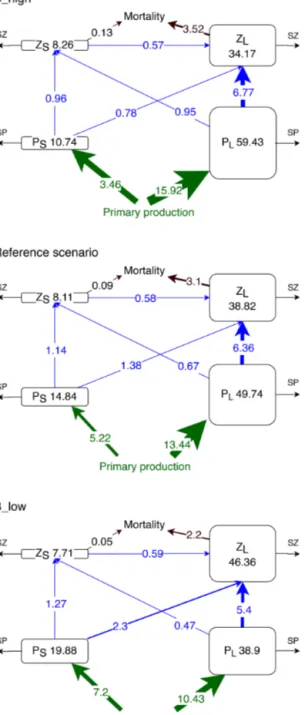
3.3 Effects on the food web in the coastal domain An increase in zooplankton mortality causes only small changes in total primary production in the coastal upwelling region (C), but the partitioning between the two phytoplankton groups changes (Fig. 6). In particular, total primary productivity of the system is increased by 3.9 % in B_high and reduced by 5.5 % in B_low. Large phytoplankton is the dom-

inant group. However, its productivity increases by about 19 % in B_high and decreases by 22 % in B_low; i.e. its changes are much more pronounced than the overall phytoplankton response. Because small phytoplankton shows an inverse response in production, this dampens the change in total primary production. Thus, a low zooplankton mortality favours small phytoplankton and its growth, and a high mortality favours large phytoplankton; changes in both phytoplankton groups result in a weak response of total primary production.

Experiment B_high exhibits the highest total plankton biomass in the upper 100 m of the upwelling system (112.6 mmol N m⁻², Fig. 6), which is mostly concentrated in the large phytoplankton compartment (59.43 mmol N m⁻²).

In this experiment the main pathway of nitrogen transfer to large zooplankton is via its grazing on large phytoplankton (6.77 mmol N m⁻²d⁻¹). As mortality decreases, small phytoplankton and large zooplankton gain biomass. Large phytoplankton grazing remains the main nitrogen source for large zooplankton. However, large zooplankton consumption of small phytoplankton is almost 3 times higher in B_low than in B_high (Fig. 6). Thus, a reduction in mortality causes a switch in the diet of large zooplankton, from mainly large phytoplankton to a diet that consists of more than one-quarter small phytoplankton.

Small zooplankton biomass decreases by ∼ 0.4 mmol N m⁻² (about 5 % of the reference value) in B_low, but it only increases by 0.15 mmol N m⁻² (about 2 %) in B_high (Fig. 6). Despite the changes in small zooplankton biomass, the consumption of its biomass by large zooplankton remains approximately the same in all experiments, resulting in a higher proportional biomass loss of small zooplankton in scenario B_low. Hence, predation by large zooplankton as well as competition for food negatively affects small zooplankton. Under high mortality conditions, the availability of large phytoplankton as food increases (Fig. 6). However, small phytoplankton, the preferred prey of small zooplankton, declines as explained above. Such

(9)

Figure 6. Concentrations (mmol N m⁻²) and nitrogen fluxes (mmol N m⁻²d⁻¹) between plankton compartments (small and large phytoplankton P_S and P_L and small and large zooplankton Z_SandZ_L, respectively) integrated over the upper 100 m or up to the seafloor if shallower than 100 m and averaged over latitude and longitude in the coastal upwelling region (see Fig. 1). SZ and SP indicate the sinks which include phytoplankton mortality, zooplankton metabolism, large phytoplankton sedimentation, unassimilated primary production and unassimilated grazing (Gutknecht et al., 2013a).

Figure 7. Percentage normalised difference in the nitrogen flux from large and small zooplankton to detritus due to zooplankton mortality, integrated over the upper 100 m of the water column, between experiment B_high and experiment B_low and the reference scenario (see Fig. 3 for the reference scenario).

antagonistic effects on small zooplankton buffer its response in this scenario.

3.4 Zooplankton losses due to mortality response In this section, we describe the response of the nitrogen loss due to mortality, also referred to as the quadratic mortality term (µ_Z_i· [Z_i]²; see Eqs. 5 and 6). The integratedµ_Z_i· [Z_i]² in the reference scenario was provided in Sect. 2.4, Fig. 3. In experiment B,µ_Z_S· [Z_S]²andµ_Z_L· [Z_L]² exhibit different behaviours. In the coastal upwelling region, bothµ_Z_S· [Z_S]² andµ_Z_L· [Z_L]² increase in B_high and decrease in B_low (Fig. 6). However, the relative response of µ_Z_L· [Z_L]² is mild and fluctuates between±30 % outside the oligotrophic area (Fig. 7). In contrast,µZ_S· [ZS]²exhibits a clear relative increase all over the domain in B_high, and a decrease in B_low. The moderate response of large zooplankton loss can be attributed to the combined effects of changes in zooplankton concentration ([ZL]) and changes in the mortality parameter (µ_Z_L), which we varied by±50 % in this study. Large zooplankton concentration increases whenµ_Z_L is decreased, and vice versa. This opposite trend buffers the effect of a change inµ_Z_L. On the other hand, small zooplankton concentration ([Z_S]) changes in the same direction asµ_Z_S, due to the combined effects of changes in its concentration, due to grazing pressure exerted by large zooplankton and competition for food with this group, and changes inµ_Z_S.

(10)

To summarise, increasing and decreasing zooplankton mortality by 50 % generates a rearrangement of the plankton ecosystem; however, the overall changes in the large zooplankton loss are not as high as would be expected from a change in the mortality rate alone. This might buffer the system once the biogeochemical model is coupled to a model of higher trophic levels.

4 Discussion

4.1 Constraining the zooplankton compartment An increasing need for the development of end-to-end models has generated interest in using results of biogeochemical models as forcing for higher-trophic-level models (fish, macroinvertebrates and apex predators) (see Tittensor et al., 2018, for a review). In a one-way coupling set-up, the biomass of plankton available as food for higher trophic levels has been adjusted during calibration of the latter, reduc- ing the amount of plankton that is available for fish consumption (e.g. Oliveros-Ramos et al., 2017; Travers-Trolet et al., 2014b). However, for two-way coupling set-ups, this adjustment of the available plankton biomass could buffer the effect of higher trophic levels on lower trophic levels (e.g. Travers-Trolet et al., 2014b). Biogeochemical models can produce a wide range of output depending on their parameter values (Baklouti et al., 2006) and their non-linearity.

For example, a quadratic zooplankton mortality exacerbates the reduction in zooplankton biomass when concentrations are very high and prevents its extinction at very low concentrations. In addition, the multiple-resource form of the Holling type-II grazing function allows the predator to mod- ify its grazing preference towards the most abundant prey (Fasham et al., 1999). Finally, Lima et al. (2002) noted that coupled physical and food web models can transition from equilibrium to chaotic states under even small changes in their parameters. Few studies have aimed to understand such behaviour (Baklouti et al., 2006) and examined the sensitivity of the model to parameters (Arhonditsis and Brett, 2004;

Shimoda and Arhonditsis, 2016). Our model study was partly motivated by the uncertainty associated with the zooplankton mortality. Indeed our model showed that a small alteration in the mortality parameter (small compared to the wide range of values that have been used for this parameter in different biogeochemical models) can strongly affect the mass flux within the simulated ecosystem. Hence, there is an increasing need for accurate plankton representation in biogeochemical models without dismissing other compartments, such as nutrients or oxygen. Nevertheless, lack of data for validation especially of higher trophic levels is a common problem for biogeochemical models of the northern Humboldt Up- welling System (Chavez et al., 2008). Oxygen, chlorophyll and nitrate in our model have been evaluated previously (Jose et al., 2017). Here we presented the first attempt to compare

the large zooplankton compartment of the ROMS–BioEBUS ETSP configuration with mesozooplankton observations.

At the surface, zooplankton concentrations simulated by our model in the reference scenario are 1 order of magnitude higher than observations at most stations. However, sampling in the upper 10 m depth may be impacted by water disturbance by the ship adding additional errors to the measurements. The match to observations improves with depth. Modifying the mortality rate by+50 % (−50 %) produced only a change of−12 % (+19 %) in large zooplankton concentration, indicating that either the induced changes in mortality rate were not large enough or this parameter is not overly influential in improving the model fit to observations. Systems with a non-density-dependent, or linear, mortality rate respond to perturbations in a “reactive” way, as defined by Neubert et al. (2004), drifting away from equilibrium, in contrast to systems with density-dependent closure terms which tend to buffer the perturbations (Neubert et al., 2004). Therefore, we might have expected a stronger impact if we had manipulated the linear closure term of the model, or metabolic losses (see Sect. 2.2.2), rather than the quadratic term. For an average nitrogen flux due to large zooplankton mortality of 2.2, 3.1 and 3.52 mmol N m⁻²d⁻¹and large zooplankton integrated concentrations of 46.36, 38.82 and 34.17 mmol N m⁻²in the coastal upwelling region (see Sect. 3.3), the mortality rate would be 0.04, 0.08 and 0.1 d⁻¹ in scenarios B_low, reference and B_high, respectively. In all cases the values are lower than the 0.19 d⁻¹ estimated by Hirst and Kiørboe (2002) for copepods in the field at 25^◦C. The closest scenario to observations is B_high where the mortality rate is only about half of the estimate by Hirst and Kiørboe (2002). This is also the scenario that better re- sembles mesozooplankton observations, since it exhibits the lowest concentrations. On the other hand, the mortality rate estimated for the reference scenario (0.08 d⁻¹) is closer to the 0.065 d⁻¹ estimation by Hirst and Kiørboe (2002) at 5^◦C.

This is considerably lower than the temperature in our modelled region (see Fig. 1). Note, however, that zooplankton mortality in our model does not depend on temperature.

Some part of the mismatch between model and observations might be related to how both data types are generated.

Therefore, a direct comparison between model and observations has to be viewed with some caution. In our model, large zooplankton acts as a closure term which is adjusted to balance the biomass and nitrogen flux to other compartments and does not resemble a specific set of species. Its parameters (maximum grazing rate, feeding preferences, etc.) are meant to represent larger, slow-growing species with a preference for diatoms. As such, they might not be directly comparable to the observed groups. The observations, on the other hand, are susceptible to sampling errors such as net avoidance and do not cover the whole taxonomic and size spectrum of mesozooplankton. For instance, no gelatinous organisms are accounted for, which may account for an im- portant fraction of the wet biomass (Remsen et al., 2004);

(11)

only mesozooplankton greater than 500 µm is considered in the sampling (Kiko and Hauss, 2019); and fragile organisms, such as Rhizaria, are not quantitatively sampled by nets (Biard et al., 2016). Therefore, the observations might be bi- ased low in comparison to the model. Furthermore, a lack of an explicit size term in the model limits a direct comparison with observations because these depend on the mesh size of the sampling net. Finally, given the above-mentioned rather pragmatic parameterisation especially of zooplankton growth and loss rates, it is very likely that the model could be improved by a tuning or calibration exercise that targets a good match between observed and simulated zooplankton concentrations. Both the mortality estimation by Hirst and Kiørboe (2002) and the zooplankton observations in the field suggest that further tuning of the model should lean towards higher mortality rates. Nevertheless, this may require the further tuning of other parameters. Despite the complexity of the model, the considerable uncertainty in model parameters and the sparsity of observations that can constrain these parameters, this is a complex task (see e.g. Kriest et al., 2017).

Therefore, we have refrained from this effort for the present but aim at providing a better-calibrated model in the future.

The spatial variability between different profiles of zooplankton is greater in the observations than in the model, and the variability in concentrations within each single pro- file is much larger than the differences between the modelled mortality scenarios (Fig. 2). Several sources of variability are not accounted for in the model as it only simulates the most relevant processes in the system. We employ a climatological model which aims at simulating the average dynamics over several years, dismissing interannual variability. Fur- thermore, we here compare a 3-month average from January to March, while observations provide only a snapshot of a highly dynamical system. In addition, we only compared our simulated zooplankton against night observations because in our model zooplankton is always active at the surface. In reality, zooplankton is known to perform diel vertical migrations (DVMs), which could increase the export flux to the deep ocean (Aumont et al., 2018; Archibald et al., 2019; Kiko and Hauss, 2019; Kiko et al., 2020). The lack of DVM could affect the export of organic matter to greater depths and therefore the biogeochemical turnover at the surface. Zooplank- ton likely also experiences lower mortality at depth (Ohman, 1990); however, off Peru these benefits might be counter- balanced by reduced oxygen availability and the concurrent metabolic costs. These obstacles for comparing zooplankton models with observations had already been described by Mullin (1975) more than 4 decades ago: (a) “the zooplankton is a very heterogeneous group, defined operationally by the gear used for capture rather than by a discrete position in the food web” (Mullin, 1975). (b) Zooplankton is irregularly distributed in space, not necessarily following physical fea- tures. (c) Adult stages of some zooplankton groups perform vertical migrations (Mullin, 1975).

To summarise, some biases and mismatches between model and observations remain; given the uncertainties and episodic nature associated with the observations and their correspondence to their model counterparts, further studies will be necessary to more precisely calibrate the model. For a complete model evaluation, however, the small zooplankton compartment should also be evaluated against microzooplankton samples. The high mortality scenario, B_high, is the one that is closest to the observations, due to producing the smallest concentrations of large zooplankton at the surface.

However, changing this parameter was obviously not enough to match the observations. In fact, in our model an increase of 50 % in the mortality rate produced only an increase of 14 % (0.4 mmol N m⁻²d⁻¹) in large zooplankton mortality loss (see Sect. 3) because of the high non-linearity of the model. Indeed, potential changes in zooplankton losses of 5 mmol N m⁻²d⁻¹, derived by fluctuations in anchovy stocks and grazing pressure (see Sect. 1), point towards much larger values for the mortality rate. An even stronger increase in the zooplankton mortality rate (e.g. Lima and Doney, 2004, applied a 5-times-larger value), along with a subsequent adjustment of other parameters, may be necessary to approach observed values. In addition, complementary observations with other sampling methods could provide a better estimation of mesozooplankton concentrations for tuning the model.

4.2 Zooplankton mortality and the response of the pelagic ecosystem

Our model study showed the strongest response of the ecosystem to changes in the mortality rate in the highly productive coastal upwelling. Here, the response of the model ecosystem was mainly driven by large zooplankton. This can be concluded from the close similarity of model solu- tions A_high and B_high, as well as of A_low and B_low (see Appendix D). The mortality term for small zooplankton played a lesser role; in addition to the direct effect of the mortality rate, this compartment was also affected by grazing by, and competition with, large zooplankton. Large zooplankton fluctuations due to mortality directly affected large phytoplankton through grazing. Small phytoplankton, on the other hand, was affected by grazing but also by competition with large phytoplankton. Changing the mortality rate produced little effect on the mass loss of large zooplankton due to mortality; however, it altered the nitrogen pathways along the trophic chain and ultimately the concentrations of most plankton groups, albeit in different ways, depending on the direction of change. Under conditions of high zooplankton mortality the food chain is dominated by nitrogen transfer from large phytoplankton to large zooplankton, the classical food web attributed to highly productive upwelling systems (Ryther, 1969). When zooplankton mortality is reduced, large zooplankton increases its consumption of small phytoplankton, taking over the role of small zooplankton.

(12)

In our model, large zooplankton has a competitive advantage by feeding on its competitor, small zooplankton, a strategy that was also found to evolve in simple ecosystem models as an advantageous alternative to direct competition (Cropp and Norbury, 2020). We find that under low mortality conditions, this advantage increases. The importance of competition is further evidenced in the changes in small phytoplankton concentrations in the coastal upwelling region.

These were partly driven by changes in the availability of resources arising from fluctuations in large phytoplankton concentrations, which constitute the dominant group in the coastal upwelling. Natural selection, competitive exclusion and different resource utilisation strategies, together with bottom-up forcing by the physical processes in the environ- ment, can shape the plankton community in global models (Follows et al., 2007; Dutkiewicz et al., 2009; Barton et al., 2010) and indicate bottom-up effects on the phytoplankton community. On the other hand, Prowe et al. (2012) showed that variable zooplankton predation can increase phytoplankton diversity by opening refuges for less competitive phytoplankton groups and thus exert top-down effects. In our study, the biological interactions between two phytoplankton groups, mainly competition for resources (bottom-up), are additionally affected in a top-down manner by changes in zooplankton concentrations.

The processes driving the ecosystem response in our regional study are dominated by trophic interactions among the size classes of phytoplankton and zooplankton. We found a top-down-driven response affecting mainly the plankton compartments of the model. The direction of the total zooplankton and total phytoplankton change is determined by the large zooplankton and large phytoplankton groups.

Small zoo- and phytoplankton buffer the response when they present opposite trends to their larger counterparts (Table 1).

In the following, we will compare our results with a similar study by Getzlaff and Oschlies (2017).

Getzlaff and Oschlies (2017), in their sensitivity study, modified the zooplankton mortality by ±50 % in a global biogeochemical model with a spin-up time of 300 years.

Their model has only one zooplankton size class with a quadratic mortality term. For their analysis, Getzlaff and Os- chlies (2017) evaluated three regions: the whole domain, also referred to here as “global”; the region from 20^◦S to 20^◦N which in this coarse-resolution model is mainly an oligotrophic region and is referred to as “tropics”; and the region south of 40^◦S where nutrient concentrations are high and is named “Southern Ocean”. After the model spin-up, global zooplankton biomass changes by about−(+)5 %, and phytoplankton biomass by about+(−)1 % in the high (low) mortality scenario (Getzlaff and Oschlies, 2017, their Fig. 2).

In contrast, in our study, total zooplankton averaged over the full domain decreases (increases) by−11 % (10 %), and total phytoplankton changes by about+(−)6 % in the high (low) mortality scenario (Fig. 4 and Table 1). Hence, the effects of changing zooplankton mortality follow the same trend in

Table 1.Qualitative comparison of the response of total, large and small zooplankton (Z_T,Z_L,Z_S) and phytoplankton (P_T,P_L,P_S) to a 50 % higher and lower zooplankton mortality parameter in our experiments B, with the results from Getzlaff and Oschlies (2017) (Z_GO,P_GO). Full, oligotrophic and coastal upwelling refer to the regions in our study (see Fig. 1) integrated over the upper 100 m;

global, Southern Ocean and tropics refer to the study by Getzlaff and Oschlies (2017, their Figs. 2 and 3 at year 300). We grouped together global and full because both refer to the whole model domain in each of the two studies. Similarly, oligotrophic and tropics refer to regions characterised by low nutrient concentrations, and coastal upwelling and Southern Ocean are both regions with high nutrient concentrations.

ZT PT ZL PL Z_S P_S Z_GO P_GO Full and global

High − + − + − − − +

Low + − + − − + + −

Oligotrophic and tropics

High − + − + − + − −

Low + − + − + + + +

Coastal upwelling and Southern Ocean

High − + − + + − + +

Low + − + − − + − −

both studies, but they are slightly milder in the study by Get- zlaff and Oschlies (2017). At the regional scale, the responses in the study of Getzlaff and Oschlies (2017) have a feedback from lower trophic levels, either to phytoplankton in the nutrient-replete region or all the way to nutrients in the oligotrophic region. Therefore, the biomass of both zooplankton and phytoplankton is ultimately bottom-up affected. This is evidenced by a change in zooplankton and phytoplankton concentrations in the same direction (Getzlaff and Oschlies, 2017, their Fig. 3). On the other hand, although our study also exhibits a feedback from phytoplankton to zooplankton, the strongest driver remains the top-down predation of zooplankton on phytoplankton (Table 1).

The regional differences between our study and that by Getzlaff and Oschlies (2017) can likely be explained by the different model structures and experimental set-ups, namely the number of phyto- and zooplankton compartments, different timescales considered for model simulation and analysis, and the spatial domain: while Getzlaff and Oschlies (2017) applied a global biogeochemical model with just one size class of phyto- and zooplankton, simulated until near a steady state, our regional model study applies a more complex biogeochemical model with a strong seasonal cycle (see Ap- pendix C), simulated for only 30 years and constantly forced at the boundaries. Further, the short few-year timescale of our model simulations might have prevented the effects of changed zooplankton mortality from propagating to deeper

(13)

water layers which contain the largest concentrations of nutrients. Finally, the region modelled in our study is spatially already very dynamic at the mesoscale resolution, as evidenced by well-defined plankton spatial succession from the coast of the continent towards the open ocean. The phytoplankton bloom, which develops closest to the coast and then is offset while water is transported offshore, can be explained by an imbalance between sources and sinks, triggered by changing environmental conditions. For example, Irigoien et al. (2005) applied the concept of “loopholes”, proposed by Bakun and Broad (2003) to explain fish productivity and re- cruitment success, to phytoplankton: according to their concept, phytoplankton blooms are formed when environmental conditions open a loophole in the plankton community of a mature ecosystem. Then, particularly phytoplankton species that are able to escape microzooplankton predation are those that will take advantage of the loophole and bloom (Irigoien et al., 2005). Our model results suggest that similar processes occur. Low concentrations of large zooplankton allow large phytoplankton to bloom near the coast. While the water is advected offshore, zooplankton growth and grazing offset the bloom. Observations by Franz et al. (2012) also reported spatial succession with large diatoms abundant in the coastal upwelling region being replenished by nanophytoplankton offshore. However, they propose silicate as the limiting nutrient offsetting the diatoms’ peak, which is not present in our model. Furthermore, such succession is not unique to the NHCS but a characteristic feature of upwelling regions (Hutchings, 1992). We note that in the present configuration the BioEBUS model does not include any temperature- dependent zooplankton grazing rate. We expect that, if this were implemented, the loophole for phytoplankton growth in the cold waters of the coastal upwelling region would even be widened, amplifying the spatial succession we observed. However, temperature might also affect zooplankton metabolism, with colder temperatures decreasing its loss rates, which could in turn mute these effects again. On the other hand, the global model by Getzlaff and Oschlies (2017) does not resolve mesoscale processes. Furthermore, while they divided their study into the tropics, as an oligotrophic region, and the Southern Ocean, as an upwelling region, the upwelling system off Peru in the eastern tropical South Pa- cific is a nutrient-rich area. For all of this, we based our comparison on similarities in the nutrient concentration (high nutrients, oligotrophic and whole domain), rather than on geo- graphic overlap.

In Getzlaff and Oschlies (2017), the zooplankton loss due to mortality is not provided. However, it can be calculated from the zooplankton concentration and mortality rate. Assuming integrated zooplankton biomasses at year 300 (Getzlaff and Oschlies, 2017, their Fig. 2) of 98, 93 and 89 Tg N in the low mortality, reference and high mortality scenarios, respectively; mortality parameters of 0.03, 0.06 and 0.09(mmol N m³)⁻¹d⁻¹; and a quadratic mortality term, then there is a difference of−44.5 % and 37.4 % in the zoo-

plankton loss due to mortality between the low and reference scenario and between the high and reference scenario, respectively. As shown in Sect. 3.4, the mortality rate in our study is also smaller than the±50 % changes that would be expected from a change in the mortality parameter of±50 % (see Sect. 2.4). The non-linearity of both global and regional models seems to reduce the effect of changes in the mortality parameter on zooplankton loss.

In summary both studies show a similar global response to changes in zooplankton mortality, driven by zooplankton preying on phytoplankton. Two zooplankton and phytoplankton size classes present opposite trends in our studies, buffer- ing the overall response. Nevertheless, the relative changes in total zooplankton and total phytoplankton are on the same order of magnitude as in Getzlaff and Oschlies (2017) and even slightly higher. Regionally different feedbacks operated in the two models, possibly due to the specific set-up of each study, spin-up time and resolution. Finally, the relative change in the zooplankton loss due to mortality is smaller than the expected±50 % in both studies.

4.3 From plankton to higher trophic levels

In our study, we changed the zooplankton quadratic mortality, which could be regarded as the effect of a predator tar- geting highly aggregated zooplankton populations, or whose concentration closely follows that of zooplankton. This can be viewed as a way to parameterise the effect of changing fish abundance on the biogeochemistry of the system. In this case, a low zooplankton mortality implies fewer small pelagic fish (such as anchovies and sardines), while a high zooplankton mortality implies a higher abundance of such fish. Further, our experiments are based on two different assumptions: one where small pelagic fish feed only on large zooplankton (experiments A) and one where they feed on and affect the mortality of both large and small zooplankton (experiments B).

The diet of anchovy is still under debate. While previ- ous studies had considered that anchovies feed mainly on phytoplankton, Espinoza and Bertrand (2008) concluded that anchovies feed on zooplankton, especially euphausiids and copepods. Furthermore, the diet of anchovy seems to be more flexible than previously considered (Espinoza and Bertrand, 2008). For instance, the anchovy collapse in 1972 was corre- lated with a shift from a population feeding mostly on phytoplankton to a southern population feeding on zooplankton (Hutchings, 1992). On the other hand, small zooplankton groups such as ciliates have been reported as a minor com- ponent of anchovy diet (Table 5 in Espinoza and Bertrand, 2008). Thus, experiments A are more likely to resemble the fluctuations in anchovy populations. On the other hand, sardines, with their finer gill rakers, obtain most of their nu- trition from microzooplankton (van der Lingen et al., 2006).

Although currently sardines are not as abundant as anchovies off Peru, historically they have also built up large concen-