What are Marine Ecological Time Series telling us about WKH}RFHDQ"

(1)

Technical Series 129

What are Marine Ecological Time Series telling us about WKH}RFHDQ"

A STATUS REPORT

Intergovernmental Oceanographic Commission United Nations

(GXFDWLRQDO6FLHQWL¿FDQG Cultural Organization

(2)

Intergovernmental Oceanographic Commission of UNESCO (IOC-UNESCO)

UNESCO’s Intergovernmental Oceanographic Commission (IOC), established in 1960, promotes international cooperation and coordinates programmes in marine research, services, observation systems, hazard mitigation, and capacity development in order to understand and effectively manage the resources of the ocean and coastal areas. By applying this knowledge, the Commission aims to improve the governance, management, institutional capacity, and decision-making processes of its 148 Member States with respect to marine resources and climate variability and to foster sustainable development of the marine environment, in particular in developing countries.

Disclaimer

The designations employed and the presentation of the material in this publication do not imply the expression of any opinion whatsoever on the part of the Secretariats of UNESCO and IOC concerning the legal status of any country or territory, or its authorities, or concerning the delimitation of the frontiers of any country or territory.

The authors are responsible for the choice and the presentation of the facts contained in the publication and for the opinions expressed therein, which are not necessarily those of UNESCO and do not commit the Organization.

For bibliographic purposes, this document should be cited as:

O’Brien, T. D.¹, Lorenzoni, L.², Isensee, K.³, and Valdés, L.⁴ (Eds). 2017. What are Marine Ecological Time Series telling us about the ocean? A status report. IOC-UNESCO, IOC Technical Series, No. 129: 297 pp.

1 National Oceanic and Atmospheric Administration (NOAA), Silver Spring, Maryland, United States

2 University of South Florida (USF), St. Petersburg, Florida, United States

3 Intergovernmental Oceanographic Commission of UNESCO (IOC-UNESCO), Paris, France

4 Instituto Español de Oceanografía (IEO), Santander, Spain

Copyright pictures on front cover (from right to left):

Kirsten Isensee, Maria Grazia Mazzocchi, James R. Wilkinson SIO-CalCOFI, Digna Rueda

What are Marine Ecological Time Series telling us about the ocean? A status report

is available online in electronic format at:

http://ioc.unesco.org

(3)

Intergovernmental Oceanographic Commission

What are Marine Ecological Time Series telling us about the ocean?

A status report

Editors:

Todd D. O’Brien Laura Lorenzoni Kirsten Isensee Luis Valdés

With the support of the Korea Institute for Ocean Science and Technology (KIOST)

T echn ica l S e ri es 129

(4)

Foreword

Some of most valuable scientific discoveries and some of the most beautiful and iconic illustrations in en- vironmental sciences (e.g. the Keeling Curve

¹

) were only possible thanks to the data obtained by long‐term systematic observations – the so called Time Series‐ of natural events and conditions. Such time series have been carried out to discover facts about them and to formulate laws and principles based on these facts.

Data provided by ship-based biogeochemical and ecological ocean time‐series provide the information to quantify the rate and range of variability of many oceanographic parameters, environmental variables and biological communities. These time series enable estimates of the rate of ocean warming and the effects of global change on the ecosystem processes, e.g. production and sedimentation. They provide reference base- lines that are essential to define the extent of environmental disturbances and estimate recovery times. In short, the time series are instrumental in providing the data required to describe, characterize, and quantify the cycles, patterns, variability, and trends of the marine environment and its biota.

Almost since its foundation, the Intergovernmental Oceanographic Commission of UNESCO (IOC‐

UNESCO) has promoted and advocated for the establishment of ocean observatories. However, it was only in 2013 that the IOC‐ UNESCO decided to support the International Group for Marine Ecological Time Series (IGMETS) as a result of synergistic activities of the Ocean Carbon and Biogeochemistry Program (OCB), the International Ocean Carbon Coordination Project (IOCCP), and the International Council for the Exploration of the Sea (ICES), with generous funding provided by the Republic of Korea. This initiative aims to aggregate and analyse the existing biogeochemical and ecological time series distributed around the world in an effort to augment the observing power to look at changes within different ocean regions, to explore plausible reasons for their similarities and differences, and to seek connections in the driving forces at ocean basin and global scale. The global perspective will highlight locations of especially large changes that may be of particular ecological importance.

In a first step, IGMETS identified and compiled the metadata from a large number of ship-based biogeo- chemical and ecological ocean time‐series that are currently conducting regular measurements. This exer‐

cise ‐as if we were following a treasure map ‐ resulted in the identification of many existing time series which now comprise part of IGMETS and their locations are displayed in a graphical world map

²

with the metadata accessible in the IOC website. The experts engaged with IGMETS, including the IOC Secretariat, were strongly motivated and convinced that the collective value of these data is greater than that provided by each time series individually. Because the individual time series are distributed across different oceans and managed by different countries, collaboration with countries’ institutions conducting the time‐series was essential. Their aggregation and synthesis would provide a quantum jump in regional and global ocean ecosystem science. This was how this publication came about.

The statistical analysis and writing process was a rewarding process. We realized very soon that if we

wanted to use the existing time series to predict future changes or drifts in the ecosystem dynamics we had

to overcome obstacles like the limited number, the non-uniform dispersion, and variable length of the time

series themselves. The message was clear: more sampling sites and much longer series are needed in order

to gain statistical accuracy if the data are to be used for a plausible prognosis.

(7)

Another realization that occurred over and over again in the IGMETS discussions was that, in spite of their scientific value and relevance, long‐term monitoring programmes are often heavily dependent on the per‐

sonal effort and dedication of individual scientists whose tenure is finite. Thus, many sampling pro- grammes are abandoned after a few years. It is hard to understand why it has proved to be so difficult to establish sustained long‐term environmental monitoring programmes. In some cases, it is due to the reluc‐

tance from funding agencies to commit long‐term support for projects that are constantly seen as “work in progress” and/or treated as “repetitive monitoring”. Hopefully this situation will reverse in the near future, as the environmental pressures the ocean is facing and the associated information needs (e.g. Climate change and the UN Sustainable Development Goals) are largely dependent on dedicated and widely dis- tributed observation networks and therefore more long‐term monitoring projects should be established worldwide.

With this report, the Intergovernmental Oceanographic Commission of UNESCO is showcasing the im- portance of the ship‐based biogeochemical and ecological time series as one of the most valuable tools to characterize and quantify ocean ecosystems. These results are intended to encourage other colleagues and their institutions to establish new time series and/or continue the sustained systematic sampling of the existing ones and promote data sharing.

The preparation of the report was only possible thanks to the colleagues that run the time-series pro- grammes across different oceans, month after month and year after year, and who generously gave us access to their data. We gratefully acknowledge all of them. I would like to thank my fellow IGMETS mem- bers for their commitment, talent, and hard work to summarize the existing, fragmented science, and as- semble and make sense of the time series used in this analysis. I also want to thank everyone who contrib- uted to the reviewing and editing of this volume for their dedication and time. Working together, a com- prehensive assessment has been produced of ocean biogeochemical and ecological knowledge that demon- strates the scientific potential of ship-based and ecological ocean time‐series around the world.

Luis Valdés

(8)

Preface

(placeholder … coming soon)

(9)

Guide to the Report

This section describes the format of the IOC-UNESCO Technical Series 129 Report and its chapter’s structure. The report was peer reviewed by experts specializing in the different regions of the ocean addressed within the report. The report was written for an audience with a certain level of scientific knowledge, with exception of the Executive Summary, which is designed to be accessible to a broader audience.

Executive Summary

The Executive Summary describes the major findings of this report, the IOC-UNESCO Technical

Series 129 Report “What are Marine Ecological Time Series telling us about the ocean? A status

report”, and highlights some of the significant points of each chapter.

Introduction, Methodology and Ocean Basin Chapters

A general introduction, highlighting the purpose of and scientific questions behind this report, is followed by a section describing the methodology applied in the ocean basin chapters. These chap- ters include key findings, which are based on the authors’ analysis of the available time‐series data and scientific, peer‐reviewed literature from that region. The time-series analysis in this report only considers data through the end of 2012. This time gap was necessary to ensure that the participating institutions/time-series sites had sufficient time to process their samples (especially plankton counts) and to complete verification of their data. In brief, the results presented herein provide an overview of information from time‐series sites and describe general hydrographic, climatic, and biological characteristics and trends, as well as changes over different time scales. Additional anal- yses integrate relationships to major climatic indices for the different ocean basins.

The order of the chapters follows the ocean conveyor belt (thermohaline circulation), starting up north with the Arctic Ocean, followed by the North and South Atlantic Ocean, subsequently ana- lyzing time‐series information in the Southern, Indian, South Pacific and finally North Pacific Ocean. The Global Chapter aims at understanding connections between ocean basins and assessing changes at a larger, global scale.

Annex

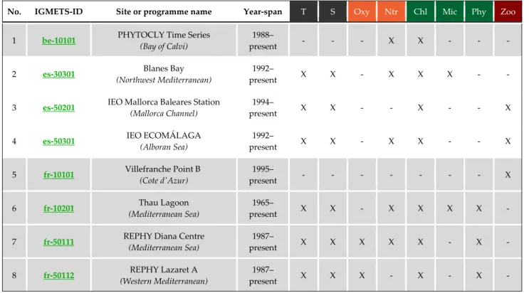
The Annex includes detailed information about the time‐series sites and surveys that participated in this analysis. For each chapter, a table lists the different time‐series sites/surveys located in the ocean basin, the duration, the country conducting the sampling and analysis, and the parameter groups measured. Each site is described with a short paragraph accompanied with a geographic location map. More detailed information on all of the programmes and time series can be accessed online at http://igmets.net/metabase/.

List of Acronyms

(10)

Executive Summary

Sustained ocean observations, including ships, autonomous platforms, and satellites, are critical for monitor- ing the health of our marine ecosystems and developing effective management strategies to ensure long‐

term provision of the marine ecosystem services upon which human societies depend. Ocean observations are also essential in the development and validation of ocean and climate models used to predict future conditions. Ship‐based biogeochemical time series provide the high‐quality biological, physical and chem- ical measurements that are needed to detect climate change‐driven trends in the ocean, assess associated impacts on marine food webs, and to ultimately improve our understanding of changes in marine biodi- versity and ecosystems. While the spatial ‘footprint’ of a single time series may be limited, coupling observations from multiple time series with synoptic satellite data can improve our understanding of criti- cal processes such as ocean productivity, ecosystem variability, and carbon fluxes on a larger spatial scale.

The International Group for Marine Ecological Time Series (IGMETS) analyzed over 340 open ocean and coastal datasets, ranging in duration from five years to greater than 50 years. Their locations are dis- played in a world map (Discover Ocean Time Series, http://igmets.net/discover) and in the IGMETS information database (http://igmets.net/metabase). These cross‐time‐series analyses yielded important in- sights on climate trends occurring both on a global and regional scale.

At a global level, a generalized warming trend is observed over the past thirty years, consistent with what has been published by the IPCC (2013) report as well as other research. There are regional differ- ences in temperature trends, depending on the time window considered, which are driven by regional and temporal expressions of large‐scale climatic forcing and atmospheric teleconnections. This warming is accompanied by shifts in the biology and biogeochemical cycling (i.e. oxygen, nutrient, carbon), which impact marine food webs and ecosystem services.

The surface waters of the Arctic Ocean have been steadily warming over the past 30 years, from 1983‐2012.

Chlorophyll biomass, as determined by satellite observations, has increased slightly over the past fifteen

years, from 1998‐2012. The complexity of the Arctic marginal seas and central basin settings, and the scarcity of in situ data, limit the analysis of biogeochemical and biological community changes across the pan‐Arctic.

The first comprehensive analysis of in situ time series provided for the North Atlantic Ocean revealed that, despite being the most studied region of the global ocean, there are large areas in this region still lacking multidisciplinary in situ observations. However, over the 25‐ and 30‐year analysis periods, > 95% of the North Atlantic Ocean

significantly warmed and the chlorophyll concentrations decreased (p < 0.05). At

the same time, negative trends in salinity, oxygen and nutrients, as exemplified by nitrate, were noted.

The analysis of existing time series showed that even in adjacent areas that appear to be relatively homog- enous, there is large variability in ecosystem behaviour over time, as observed in the continental shelves at both sides of the North Atlantic Ocean.

In general, over the 5‐year period prior to 2012, ~70% of the area of the South Atlantic showed cooling

and 66% decreasing chlorophyll concentrations.

However, over the

past 30 years, > 85% of the South Atlantic increased in temperature. The paucity of in situ time series in this region, and the striking changes

that have been reported in South Atlantic ecosystems over the past two decades, highlight the need to have

a better observing system in place.

(11)

Both

long‐term trends and sub‐decadal cycles

are evident in the Southern Ocean on multiple trophic levels, and they are strongly related in complex ways to climate forcings and their effects on the physical oceanographic system. Antarctic marine ecosystems have changed over the past 30 years in response to changing ocean conditions and changes in the extent and seasonality of

sea ice. These changes have

been spatially heterogeneous which suggests that ecological responses depend on the magnitude and direction of the changes, and their interactions with other factors.

Of all the ocean basins, the

Indian Ocean

showed the greatest extent of warming, with

92% of its area showing a significant (p < 0.05) positive trend over 30 years, compared with the Atlantic (89%), the Pacific

(66%), the Arctic (79%) and the Southern (32%) oceans. In addition to having a high degree of warming, the Indian Ocean also had the greatest proportion of its area (55%) showing a significant (p < 0.05) decline

of chlorophyll

between 1998 and 2012. Given the spatial scale of warming in the Indian Ocean, it does seem likely that climate impacts on marine ecosystems will be most pronounced in this basin. The Indian Ocean has very few in situ biogeochemical time series that can be used to assess impacts of climate change on biota or biodiversity.

Over the past 30 years, significant (p < 0.05) surface warming has been recorded for 67% of the area of the

South Pacific Ocean.

A strong physical coupling with planktonic ecology and biology is evident in the South Pacific, with a dominant warming pattern and significantly declining phytoplankton populations.

The North Pacific Ocean has undergone significant changes in ocean climate during the past three decades.

Based on both satellite and ship‐based SST measurements, over

65% of its surface area has undergone significant warming since 1983 (p < 0.05). The patterns of change suggest that the PDO

has been the dominant mode of climate variability in the North Pacific Ocean

between 1983 and 2012.

However, marked variability in SST has been observed, with episodes of warming in 2002, 2004 and 2010 interspersed with periods of cooling, particularly since 2008 due to the combined effects of La Niña and a negative, cooling PDO phase.

Long‐term time series in the

central, subarctic northeast and western North Pacific Ocean show an increase in phytoplankton biomass during the past 30 years. However, satellite observations suggest that over 65% of the surface of the North Pacific has experienced a decline in chlorophyll concentration since

1998. Available time series show an increase in zooplankton biomass in the waters off Hawaii, southern Vancouver Island and the western United States during the last 15 years but an overall decrease at most other locations, with no significant correlation between zooplankton biomass and chlorophyll.

Nutrients, salinity and dissolved oxygen at the ocean surface appear to be negatively correlated with SST across the North Pacific.

The IGMETS effort highlights the value of biogeochemical time series as essential tools for assessing, and

predicting, global and regional climate change and its impacts on ecosystem services. The capacity to

identify and differentiate anthropogenic and natural climate variations and trends depends largely on the

length of the time‐series, as well as on the location. Most of the ship based ecological time series are

concentrated in the coastal ocean. While coastal zones in North America and Europe are being monitored,

there is a conspicuous lack of biogeochemical time‐series in other coastal regions around the world, and an

almost complete absence of such observational platforms in the open ocean, which limits the capacity of

analyses such as this. A more globally distributed network of time‐series observations over multiple decades

will be needed to differentiate between natural and anthropogenic variability.

(12)

(13)

Chapter 1 Introduction

1 Introduction

Luis Valdés and Michael W. Lomas

Figure 1.1. Schematic of the global thermohaline ocean circulation – conveyor belt. Blue arrows indicate generally cooler water currents and red arrows indicate generally warmer currents. The red and blue areas beneath these arrows indicate 10-year (2003–2012) sea surface temperature warming and cooling trends, as summarized in the “Methods and visualization” chapter (e.g. Figure 2.8) and used throughout this report.

1.1 Global importance of time series

The observation of nature and the understanding that there are underlying regularities (cause-and-effect relationships) dates back to the very origin of human cul- ture. In fact, this knowledge allowed for the management of natural resources and for the establishment of the earliest human settlements, e.g. the very first agricul- tural societies. The prediction of Nile flooding was critical not only for food security, but it was also a matter of political power.

There are many examples of records of long-term systematic observations of natural events and conditions from crop yields, planet movements, sun spots, river discharges, and freezing records dating from ancient

times (Bell and Walker, 2013). Many of the most beautiful scientific discoveries were possible thanks to data obtained by regular observations – time series – carried out with the purpose of discovering facts about certain phenomena and to formulate laws and principles based on these facts.¹

1To state that a particular phenomenon always occurs if certain conditions are present is a principle of conservation laws of physics, which reflects the homogeneity of a process in space and time. The search for patterns and symmetries is one of the main goals of science, and reducing uncertainties in a given phenomenon makes us feel comfortable as if we were able to reduce the entropy and minimize the occurrence, or the im-

(14)

Figure 1.2. Temporal and spatial scales of a range of ocean processes. The blue square highlights the range of space- and time-scales that can be addressed by ship-based, time-series measurements (Adapted from Dickey, 2002).

The biogeochemistry of the ocean (Figure 1.1) varies naturally across a range of temporal and spatial scales (Figure 1.2), which is often further conflated with anthropogenic forcing (warming, acidification, pollution, etc.). In a growing effort to distinguish between natural and human-induced earth system variability, sustained ocean time-series measurements have taken on a re- newed importance as they represent one of the most valuable tools that scientists have to characterize and quantify ocean ecosystem cycles and fluxes and their associated links to changing climate.

Ocean time series, particularly ship-based repeated measurements, consist of one type of observation programmes which are crucial to answering scientific questions and improving decision-making in ocean and coastal management (Edwards et al., 2010). They provide the oceanographic community with the long, temporally resolved datasets and high-quality data needed to characterize ocean physics, climate, biogeochemistry, and ecosystem variability and to change what can be used to examine, test, and refine many paradigms and hypothe- ses about the functioning of the ocean (Henson, 2014).

induced changes in marine ecosystems (Reid and Val- dés, 2011).

1.2 Levels of understanding and need for continued sampling

Time-series data help resolve both short- and long-term scales of variability, depending on sampling frequency, and provide context for traditional process-oriented studies.

Depending on motivation, sampling frequency, and length, time series can be used for different purposes (Figure 1.3) and are of critical importance to enable or facilitate: (i) the acquisition of ecosystem baselines and rate and scale of environmental change, including climate change and biodiversity loss, (ii) the understanding of ocean, earth, and climate system processes, (iii) to monitor ecosystem dynamics and its variability, (iv) the detection of hazards and environmental disturbances and the estimation of recovery times, (v) to forecast and anticipate ecosystem changes, and (vi) effective policy- making and sustainable management of the seas and

(15)

Significant advances in our understanding of ocean processes in some well-studied systems have shown that not all ocean regions are changing at the same rate or following the same pattern. This is, in part, because the ocean is characterized by interacting processes, which operate over nearly 10 orders of magnitude in time and space (Dickey, 2001, 2002). Indeed, some regions are more sensitive to environmental change than others.

Exploring this temporal and spatial variability of ocean change, at a basin-scale or greater, is largely the realm of earth ecosystem models at present. Indeed, it is only through models that we can learn about the spatial rep- resentativeness of existing time series (i.e. the footprint of a time series) and, therefore, inform decisions about where to site new time series (Henson et al., 2016).

While our understanding of first-order ocean biogeochemical concepts in these models and their coupling to atmospheric forcing is reasonably well developed (Kel- ler et al., 2014), these models are still limited by lack of mechanistic and observational knowledge in time and space of how the ocean is changing physically, chemical- ly, and biologically and, worse yet, the interactions be- tween these levels of variability (Heinze et al., 2015). This is further exacerbated by the fact that observational time series generally have to be several-fold longer than the time-scale they are trying to resolve, while models can produce multidecadal output with relative ease. For

example, published model output suggests that at least three decades would be needed to resolve climate- change response in the North Atlantic in certain variables (e.g. primary production), but less in others (e.g. sea surface temperature) (Henson et al., 2010, 2016).

Obviously, the “pay check” you receive from consistent long-term, ship-based marine time series is not regular, but many times it is surprising, as demonstrated by recent discoveries, e.g. proof of ocean acidification, ecosystem regime shifts, and exploration of the deep sea, which illustrate that sustained multidecadal observations are ecological and economical important research investments for future generations.

In a time of increasing pressures on the marine environment, time series are central to understanding past, current, and future alterations in ocean biology and to monitoring future responses to climate change (Valdés et al., 2010; Karl, 2014). With many time series now having accumulated sufficient data to quantify variability and trends (see Figures 2.2 and 2.3 in the “Methods and visualization” chapter), it would be foolish to allow reductions or long gaps in sampling to occur, and re- placing the ship-based, long-term series with autonomous platforms should not be the ultimate path to fol- low.

Figure 1.3. Representative sampling time-scales needed to establish a minimum level of understanding across levels of complexity

(16)

While these tools provide high-quality and high- frequency data for certain, generally physical and geo- chemical, parameters, ship-based time series are unique in their multidisciplinarity: physical, chemical, and biological parameters can be measured simultaneously.

Many ecosystem processes and functions (e.g. primary production, phytoplankton composition, utilization of specific nutrients) cannot be directly obtained from these autonomous sensors, and only some can be derived through proxy measurements. Furthermore, regular and consistent calibration of independent sensors, moorings, and remote-sensing techniques can only be assured with standardized in-situ measurements.

1.3 New light for time series: interna- tional collaboration in ship-based ecosystem monitoring

The history of long-term ocean time series started more than 100 years ago. In the Western English Channel and around the British Isles, records go back to the late 19th century. A broad suite of marine time-series sites was established in the middle of the 20th century in the Northern Hemisphere, e.g. Station M in the Norwegian Sea (1948), NOAA Ocean Station P Sea in the North Pacific (1947), Henry Stommel’s ‘Hydrostation S’ in the Sargasso Sea (1954), and Boknis Eck Time Series Station where monthly sampling began in April 1957 (Owens, 2014).

Many other coastal and oceanic time series were established across different oceans and managed by different countries since the 1980s and 1990s following recom- mendations from international programmes such as JGOFS (1990) and GLOBEC (1997).

The value of these measurements has not been fully appreciated, and several sampling sites face severe funding difficulties. Some could not sustain measurements with the same sampling frequency in time, resulting in temporal gaps of observations, and financial resources even ceased, and no alternatives could be obtained (Frost et al., 2006). However, many others survived and gained international prestige (e.g. HOT, BATS, CARIA- CO, ESTOC, Plymouth L4, Helgoland Roads, RADIAL- ES) particularly for providing the reference baselines for different variables at local–regional scales and in different ocean biogeographical provinces.

Difficulties in harmonizing the data, digitalizing results to enhance broad accessibility, and evaluating methods hampered the utilization of these historical datasets. As a contribution to GLOBEC, ICES encouraged the international comparison and analysis of time series, which was adopted by the ICES Working Group on Zooplank- ton Ecology (Valdés et al., 2005; O’Brien et al., 2012;

Wiebe et al., 2016) and then continued by SCOR WG125 and WG137 (WG125: Global Comparisons of Zooplankton Time Series and WG137: Patterns of Phytoplankton Dynam- ics in Coastal Ecosystems: Comparative Analysis of Time Series Observation). Now, the International Group for Marine Ecological Time Series (IGMETS; Figure 1.4), under the auspices of the IOC-UNESCO, is taking on the mantle of improving access to time series. All of these groups stressed the need to broaden the scientific utilization of existing time-series datasets and to link current and past studies.

The goals of IGMETS are to look at holistic changes in different ocean regions, explore plausible reasons and explanations at regional and global scales, and highlight locations of especially large change that might be of particular importance for model projections or ongoing management policies. In the process, IGMETS intends to aggregate existing time-series sampling sites, establish global baselines, assess spatial variability and response to climate at the basin-scale and greater, and provide the basis for projection and forecasting.

(17)

Figure 1.2. Previous and ongoing activities within the scientific community leading up to the IGMETS effort.

1.4 The ocean time series heritage

A time-series workshop in November 2012 was orga- nized by OCB, IOCCP, and IOC-UNESCO. One of the key outcomes of this workshop was the development of a global time-series network compiling more than 140 ship-based time series and to improve evaluation and coordination of methods and communication among marine biogeochemical time series. The compilation of metadata of time series continued under the IGMETS umbrella; more than 340 open ocean and coastal datasets, ranging in length from 5 to >50 years and having a similar set of minimal observations, have so far been identified. Their locations are now displayed in a world map (inner cover of this volume) and in the metadata search on the http://IGMETS.net website. These time- series sampling sites represent a phenomenal heritage legacy, and intergovernmental bodies such as ICES, European Marine Board, or IOC-UNESCO strongly recommend continuing the systematic sampling of the existing sites and establishing new time series based on the knowledge gained.

Given that individual time series are distributed across different oceans and managed by different countries, open collaboration with national institutions managing the time series is essential. Sustaining a ship-based time series requires careful planning, periodic evaluation of approach and methods (including implementation of new methods and measurements as appropriate), and a good data-dissemination policy (Karl, 2010).

IGMETS advocates:

1) Observations which are not made today are lost forever!

2) Existing observations are lost if they are not made accessible.

3) The collective value of datasets is far greater than their dispersed value.

4) No substitute exists for adequate observations.

5) The value of time-series observations is posi- tively correlated with the duration of continuous measurements. Measurements encompassing a time-span of several decades allows identification of seasonal, interannual, and decadal patterns.

6) The analysis of multiple datasets from different time-series stations allows the separation of stressors and the evaluation of connected ecosystem responses.

7) During previous decades, science and technology evolved along with time-series observations. Anticipated development of new techniques will allow streamlining the measurements and improving their geographical coverage.

8) Advanced analysis, including global assess- ments and improved computation, using existing data, creates new science.

9) Models will evolve and improve, but, without data, will be untestable – projections and forecasting require considerable diversification of in situ data.

10) Today’s climate models will likely prove of lit- tle interest in 100 years. But, adequately sampled, carefully quality controlled, and archived data for key elements of the climate system will be useful indefinitely.

(18)

1.5 Overview of this report

There are an extraordinary number of unexploited datasets obtained by long-term ocean time series. Large spatial-scale analyses using many different time series allow us to augment our capacity to detect and interpret links between climate variability and ocean biogeochemistry, ultimately improving our understanding of marine ecosystem change. However, in order to bring together datasets from different time series, it is important that the sampling and analytical protocols used at each site are homogenous, consistent, and intercomparable.

For the purposes of analyses presented in this report, we define a time series as a location that is sampled at least once per season (such that strong seasonal patterns can be removed to study lower-frequency variability). We also only examined near-surface observations. This is, in part, due to taking a global view for this analysis and thus avail ourselves of satellite observations to fill in spatial gaps between in situ observations, but also be- cause there are far fewer ecological time series that sample in the vertical domain. Within the time-series compilation records, 214 contain information on zooplankton, 142 on phytoplankton, and 145 on nutrients. Data obtained after 2012 were not included in the analysis, which allows the data owner to be the first to publish new findings in the peer-reviewed literature.

The result presented herein provide a brief overview of the information provided from the long-term time-series sites and describe general hydrographic, climatic, and biological characteristics and trends, explaining the change over time. This analysis allows for comparisons of changes occurring in distant locations and helps to detect changes occurring at broad scales and to distinguish them from local imbalances or fluctuations. Addi- tional analyses integrate relationships to major climatic indices for the different ocean basins.

Analyzing the datasets obtained at multiple ocean time- series sites has high scientific value, but sharing data has also important economic and social benefits. The de- mand from different stakeholders and decision-makers for answers to the challenges posed by changes in the marine environment is growing rapidly. Sharing and accessing time-series data would reduce uncertainties in the management of marine resources and ecosystem services.

This document reviews the dynamics and climate trends that have been reported from different ocean basins and discusses potential future changes to the ecological processes of marine systems. Forecasting the dynamics of ocean processes requires the use of mathematical models, which are often limited by data availability. Chal- lenges are highlighted in this publication in the hope that continuing research efforts will fill knowledge gaps and thus improve our ability to predict future trends and facilitate the successful management and conservation of marine species, habitats, living marine resources, and ecosystem services.

In summary, this IGMETS report aims to deliver new insights into existing biogeochemical and ecological ship-based times-series and to reduce scientific uncer- tainty regarding environmental change. The report also features an overview of the gaps and needs for better sampling coverage in the different ocean basins and seas.

(19)

1.6 References

Bell, M., and Walker, M. J. C. 2013. Late Quaternary Environmental Change: Physical and Human Perspectives. Routledge, New York. 355 pp.

Dickey, T. 2001. The role of new technology in advanc- ing ocean biogeochemical research. Oceanogra- phy, 14(4): 108–120.

Dickey, T. 2002. A vision of oceanographic instrumenta- tion and technology in the early 21st century. In Oceans 2020: Science, Trends, and the Challenge of Sustainability, pp. 209–254. Ed. by J. G. Field, G. Hempel, and C. P. Summerhayes. Island Press, Washington, DC. 296 pp.

Edwards, M., Beaugrand, G., Hays, G. C., Koslow, J. A., and Richardson, A. J. 2010. Multidecadal oceanic ecological datasets and their application in marine policy and management. Trends in Ecology

& Evolution, 25: 602–610,

doi:10.1016/j.tree.2010.07.007.

Frost, M. T., Jefferson, R., and Hawkins, S. J. (Eds). 2006.

The evaluation of time series: their scientific value and contribution to policy needs. Report prepared by the Marine Environmental Change Network (MECN) for the Department for Environment, Food and Rural Affairs (DEFRA), Marine Biologi- cal Association, Plymouth. Marine Biological As- sociation Occasional Publications No. 22. 94 pp.

GLOBEC. 1997. Global Ocean Ecosystem Dynamics (GLOBEC) Science Plan. Final editing by R. Har- ris and the members of the GLOBEC Scientific Steering Committee (SSC). IGBP Report 40. 83 pp.

Heinze, C., Meyer, S., Goris, N., Anderson, L., Steinfeldt, R., Chang, N., Le Quéré, C., et al. 2015. The ocean carbon sink – impacts, vulnerabilities, and challenges. Earth System Dynamics, 6: 327–358.

Henson, S. A. 2014. Slow science: the value of long ocean biogeochemistry records. Philosophical Transac- tions of the Royal Society A, 372: doi:

10.1098/rsta.2013.0334.

Henson, S. A., Beaulieu, C., and Lampitt, R. 2016. Ob- serving climate change trends in ocean biogeochemistry: when and where. Global Change Biol- ogy, 22(4): 1561–1571, doi:10.1111/gcb.13152.

Henson, S. A., Sarmiento, J., Dunne, J., Bopp, L., Lima, I., Doney, S., John, J., et al. 2010. Detection of anthro- pogenic climate change in the satellite records of ocean chlorophyll and productivity. Biogeosci- ences, 7: 621–640.

JGOFS. 1990. Joint Global Ocean Flux Study (JGOFS) Science Plan. JGOFS Report No 5. 67 pp.

Karl, D. M. 2010. Oceanic ecosystem time-series pro- grams: Ten lessons learned. Oceanography, 23(3):

104–125.

Karl, D. M. 2014. The contemporary challenge of the sea:

Science, society, and sustainability. Oceanogra-

phy, 27(2): 208–225,

http://dx.doi.org/10.5670/oceanog.2014.57.

Keller, K. M., Joos, F., and Raible, C. C. 2014. Time of emergence of trends in ocean biogeochemistry.

Biogeosciences, 11: 3647–3659.

O’Brien, T. D., Li, W. K. W., and Morán, X. A. G. (Eds).

2012. ICES Phytoplankton and Microbial Plank- ton Status Report 2009/2010. ICES Cooperative Research Report No. 313. 196 pp.

Owens, N. J. P. 2014. Sustained UK marine observations.

Where have we been? Where are we now? Where are we going? Philosophical Transactions of the

Royal Society A, 372:

http://dx.doi.org/10.1098/rsta.2013.0332.

Reid, P. C., and Valdés, L. 2011. ICES status report on climate change in the North Atlantic. ICES Coop- erative Research Report No. 310. 262 pp.

Valdés, L., Fonseca, L., and Tedesco, K. 2010. Looking into the future of ocean sciences: an IOC perspective. Oceanography, 23(3): 160–175.

Valdés, L., O’Brien, T. D., and López-Urrutia, A. (Eds).

2005. Zooplankton monitoring results in the ICES area, Summary Status Report 2003/2004. ICES Cooperative Research Report No. 276. 34 pp.

Wiebe, P., Harris, R., Gislason, A., Margonski, P., Skjoldal, H. R., Benfield, M., Hay, S., et al. 2016.

The ICES Working Group on Zooplankton Ecolo- gy: Accomplishments of the first 25 years. Pro- gress in Oceanography, 141: 179–201,

(20)

(21)

Chapter 2 Methods and Visualizations

2 Methods and Visualizations

Todd D. O’Brien

Figure 2.1. An example screenshot from the IGMETS time series Explorer available online at http://igmets.net/explorer and a selection of additional spatio-temporal visualizations available via the Explorer and used throughout this report.

This chapter should be cited as: O’Brien, T. D. 2017. Methods and Visualizations. In What are Marine Ecological Time Series telling us about the ocean? A status report, pp. 19–35. Ed. by T. D. O'Brien, L. Lorenzoni, K. Isensee, and L. Valdés. IOC-UNESCO, IOC Technical Series,

(22)

2.1 Introduction

With a collection of over 340 marine ecological time series, the data-assembling effort behind IGMETS was considerable (Figure 2.1). As these time series also varied in their available variables, methodologies, months of coverage, and years in length (Figures 2.2 and 2.3), a flexible yet robust analytical method was required to synthesize and compare the information. For over 12 years, the Coastal & Oceanic Plankton Ecology, Production, & Ob- servation Database (COPEPOD) been working with marine ecological time-series data assembly, analysis, and visualization when it provided the data backbone for the SCOR Global Comparisons of Zooplankton Time Series working group (WG125). COPEPOD continued its support with other time-series groups, such as the ICES

Working Group on Zooplankton Ecology (WGZE), the ICES Working Group on Phytoplankton and Microbial Ecology (WGPME), and the SCOR Global Patterns of Phy- toplankton Dynamics in Coastal Ecosystems working group (WG137).

During these years of collaboration, a suite of analytical and visualization tools has been created, modified, and expanded to support the specific needs of each of these groups (Mackas et al., 2012; O’Brien et al., 2012, 2013;

Paerl et al., 2015). These tools were again adapted and ex- panded to fit the requirements of IGMETS, creating the first-of-its-kind interactive time series visual explorer (http://igmets.net/explorer) as well as the spatio-temporal trend fields seen throughout the following chapters of the report.

TW05 sites (2008-2012) TW10 sites (2003-2012)

TW15 sites (1998-2012) TW20 sites (1993-2012)

TW25 sites (1988-2012) TW30 sites (1983-2012)

Figure 2.2. Panel of maps showing locations of IGMETS-participating time series based on time-window qualification. Red symbols indicate time-series sites with at least one biological or biogeochemical variable (i.e. excluding temperature- and salinity-only time series) that qualified for that time-window (e.g. TW05, TW20). The time-window concept and method are described in Section 2.3.2. Light gray symbols indicate sites that did not have enough data from the given time-window to be included in that analysis.

(23)

Figure 2.3. Histogram of all IGMETS-participating time series sorted by their length in years. The Continuous Plankton Recorder (CPR) time series is also plotted separately, highlighting its significant contributions to the longer time-spans.

2.2 In situ data sources

The International Group for Marine Ecological Time Se- ries effort focused on ship-based, in situ time series with chemical and/or biological data elements. IGMETS did not pursue data from buoys, floats, pier-mounted sensors, or automated underwater vehicles (AUV). With an interest in ecological time series, IGMETS most heavily pursued datasets that had chemical or biological variables (e.g. nutrients, pigments, or plankton data).

At the time of preparation of this report, more than 340 time series were participating in IGMETS. These sites are listed at the end of each chapter in the “Regional listing of participating time series” tables and are presented in more detail in the Annex of this report. The IGMETS online metabase (http://igmets.net/metabase) also includes this information and offers additional content and search tools (e.g. search by variable, length in years, pro- gramme, investigator, or country). Finally, the metabase also contains any additional time series identified and added after this initial report was published.

The term “participating time series” was used to identify time series that provided data for the IGMETS numerical analysis. Time series acknowledged in the report, but not classified as “participating”, implies that their data were not available for the analysis. Reasons for this unavaila-

The chapters of the IGMETS report are divided into larger ocean-based regions (e.g. North Atlantic, South Pacific, Arctic Ocean), separated by land masses, or, in the case of an in-water division, indicated with black dashed lines (Figure 2.4). Each regional chapter only discusses time series and trends found within that specific region. For the purpose of this report, most of the analyses and visualizations also only focused on trends within oceanic, non- estuarine sites.

2.3 Analytical methods

The IGMETS time series vary greatly in their available variables, methodologies, months of coverage, and years in length (Figures 2.2 and 2.3). A flexible yet robust analytical method was required to conduct the analyses and compare them in a meaningful way. The following sec- tions describe the methods used and the challenges addressed by the IGMETS analysis. Many of these methods are refinements and expansions of earlier work developed by COPEPOD to support other time-series working groups.

(24)

Figure 2.4. Global map illustrating the geographical boundaries of each chapter. The geographical separation of the ocean-basin chapters is set by land masses or, in the case of an in-water division, indicated with black dashed lines.

The IGMETS analysis addressed the following questions:

 How to compare time series with different methods or measuring units (Section 2.3.1),

 How to address time series with different seasonal influences (Section 2.3.1),

 How to compare time series with different time spans (Section 2.3.2),

 How to get a spatially-coherent overview from sparse data (Section 2.3.3).

2.3.1 The IGMETS statistical methodology

The comparison of variables sampled using different methods requires a careful yet flexible analysis. These differences not only include the measurement technique itself (e.g. instrumentation used, chemical method, counting method), but also sampling protocols and depth at which such measurements were collected (e.g. “surface”

vs. a bottle triggered at 10 m vs. an average of the top 10 m vs. an integration of values over the top 10 m).

Quantitatively, these values are not easily intercomparable, if at all. In terms of a time-series study, however, the focus is on how these variables are changing over time relative to themselves and to each other. Using data from different methods, one cannot necessarily intercompare how much they are changing, but it is possible to detect if

these variables are similarly increasing or decreasing over time. As long as the method used within each individual time series is consistent over the duration of that individual time series, a comparison of relative trends among multiple time series, even with different methodologies, is possible.

2.3.1.1 Calculation of trends over time

A monotonic upward (or downward) trend means that the variable consistently increases (or decreases) over time, even though that trend may or may not be linear.

Previous time-series studies by SCOR WG125 (Mackas et al., 2012) and ICES WGZE/WGPME (O’Brien et al., 2012, 2013) looked at trends by calculating the linear regression (slope) of annual anomalies within a time series. These annual anomalies were, in turn, calculated using “the Mackas method” (Mackas et al., 2001; O’Brien et al., 2013), which removed the seasonal cycle during the calculations. The Mackas method is also very tolerant of sparse data or time series with missing years or months (Mackas et al., 2001).

(25)

While the Mackas method itself was robust, ICES WGPME/WGZE found that the (parametric) linear re- gressions used to estimate trends were limited (e.g.

yielded weak p values) when accounting for the statistical complexity in some shorter ecological time series, especially those less than ten years in length. Following the suggestion of these working groups, the IGMETS time- series analysis used the non-parametric seasonal Mann- Kendall (SMK) test to test for monotonic trend in time se- ries with seasonal variation (Hirsch et al., 1982). The SMK works by calculating the Mann-Kendall score (Mann, 1945; Kendall, 1975; Gilbert, 1987) separately for each month; the sum of these values gives the final test statistic. The variance of the test statistic is likewise obtained by summing the variances of each month, and a normal approximation is then used to evaluate the significance level. IGMETS found results from the SMK to be equiva- lent to the Mackas method for time series longer than ten years and that it also frequently helped near-but-not- quite-significant shorter time series cross the “p < 0.05”

borderline.

2.3.1.2 Statistical significance

The IGMETS analyses provide tables and visualization figures that differentiate between statistically significant (p < 0.05) and non-significant trends within the in situ var- iables and satellite-based background fields. In terms of estimating the statistical significance of a monotonic trend, the calculations behind the p value depend on the:

a) number of observations (e.g. the number of years in the time series),

b) strength of the trend (e.g. the magnitude of change over time), and

c) error/variance/noise of the variable.

In terms of time series, this means:

a) A shorter time series may require a stronger trend to be considered statistically significant, while a less pronounced trend may require more years in length before being considered statistically significant.

b) A variable with a large, but natural, variance (e.g. biological or biologically influenced variables) may require more years in length and/or a stronger trend (to be considered statistically significant) than a variable with a relatively lower variance (e.g. temperature).

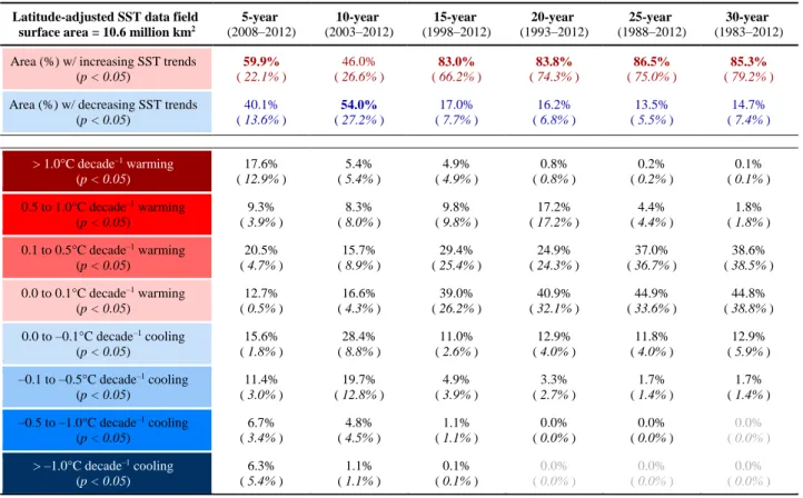
These patterns are easily seen in the “Spatial frequency”

tables (Section 2.4.4), where the ratio of significant to non- significant trends greatly increases with length of time.

Statistically significant or not, spatially coherent patterns of “increasing” and “decreasing” were evident in both temperature and chlorophyll spatio-temporal fields (Sec- tion 2.4.4 and Figures 2.8, 2.9, and 2.10).

2.3.1.3 Combined variables

Within the IGMETS variables set, a handful of related, but slightly different, variables were present. For example, some time series had chlorophyll a measurements, others had total chlorophyll, or fluorescence, and the Continu- ous Plankton Recorder (CPR) time series had data from its Phytoplankton Colour Index (PCI). As stated in the be- ginning of this section (Section 2.3.1), as long as the method used in each individual time series was consistent over the duration of that individual time series, one can compare general trends among time series, even if they used different methodologies to measure the same variable. By grouping the trends from these three methods into a loose “combined chlorophyll” category, it is possible to obtain a larger and more coherent spatial pic- ture than if only considering one method-specific variable at a time. For example, in the North Atlantic, the combined chlorophyll included the CPR PCI trends that fill the entire central transbasin North Atlantic region, an area where no chlorophyll a time series were otherwise available.

Similar combinations were done for the “combined zooplankton” grouping, which included trends from the “total copepods” abundance time series and trends from var- ious total zooplankton biomass methods (e.g. total wet weights, total dry weights, or total sample volumes). This approach has been used by SCOR WG125 as well as the ICES WGZE and WGPME plankton time-series groups (Mackas et al., 2012; O’Brien et al., 2012, 2013).

For those who wish to not combine similar variables, the IGMETS Explorer (http://igmets.net/explorer) can display the distributions and trends of time-series variables both individually and in their combined grouping forms.

(26)

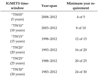
Table 2.1. Year-span and minimum year requirements for the IGMETS time-windows.

IGMETS time-

window Year-span Minimum year re-

quirement

“TW05”

(5 years) 2008–2012 4 of 5

“TW10”

(10 years) 2003–2012 8 of 10

“TW15”

(15 years) 1998–2012 12 of 15

“TW20”

(20 years) 1993–2012 16 of 20

“TW25”

(25 years) 1988–2012 20 of 25

“TW30”

(30 years) 1983–2012 24 of 30

2.3.2 IGMETS time-windows

While it is not really meaningful to compare long-term trends from a 31-year time series with a 12-year time series, it is possible to compare the 10-year trends created from the overlapping 10-year periods shared by these two time series. By splitting each time series into multiple

“time-windows” with common starting and ending dates, the IGMETS analysis looked at patterns of change over time (trends) at a variety of shared time-intervals (e.g. 5 years, 10 years, 30 years).

O’Brien et al. (2012) used a similar approach to look at 10- year and 30-year trends in major North Atlantic phytoplankton taxonomic groups. IGMETS expanded upon this approach to include 5-, 10-, 15-, 20-, 25-, and 30-year time-windows. For this study, an analysis ending date of December 2012 was selected to allow the time-series re- searchers sufficient time to process complex biological samples (e.g. complete microscope identification and enumeration of plankton samples) and to conduct any necessary quality control on their data. The IGMETS time-windows were then calculated by counting back- wards from 2012 (Table 2.1).

Table 2.1 summarizes the year span and minimum number-of-years-present requirements for the six IGMETS time-windows used in this report. Using this criteria, a time series with data for 2007–2012 would be eligible for the 5-year (TW05) time-window, but none of the longer windows. A time series encompassing 1981–2012, with no missing years, would be eligible for all six time-windows.

To ensure that a minimum number of years of data were available for statistical-trend calculations within each time-window, it was required that 80% of the years within the time-window must have data present to qualify for that window. For example, a time series with ten years of data from 2001 to 2010 could qualify for the 10- year (TW10) time-window, but would not qualify for the 5-year time-window as it only had data for three of the required four TW05 years (e.g. 2008, 2009, and 2010 are present, but 2011 and 2012 are both missing). In this example, if data for 2011 or 2012 could also be added, the time series would then qualify for the 5-year (TW05) window. Adding values for both 2011 and 2012 together would also allow this time series to participate in the 15- year time-window, as it would now have the 12 years minimum required by TW15. Under this criterium, a “60- year” time series from 1950 to 2010, but missing data every other year, would fail to qualify for any of the IGMETS time-windows.

2.3.3 Calculation of spatio-temporal trend fields

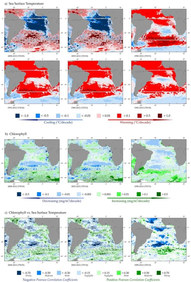
Within some oceanic regions, participating time series were sparse or simply did not exist (e.g. upper Indian Ocean and South Atlantic, central South Pacific). Even within data-rich regions like the North Atlantic, the available sites still often had vast areas with no information (Figure 2.2). While IGMETS is focused on in situ, ship- based measurements, satellite data were used to create globally covered, spatially complete fields that could shed light on the general physical (e.g. sea surface temperature) and biological (e.g. surface chlorophyll) changes that occurred during the different IGMETS time- windows.

The IGMETS spatio-temporal analysis used temperature data from the NOAA Optimum Interpolation Sea Surface Temperature dataset (OISST version 2.0, https://www.ncdc.noaa.gov/oisst) and chlorophyll data from the ESA Ocean Colour CCI dataset (OC-CCI version 2.0, http://www.esa-oceancolour-cci.org/). Both datasets were acquired in a prepared-product form, downloaded as a regular global grid of monthly mean values by year.

By using these preprepared products, the typical con- cerns and issues with satellite data (e.g. instrument inter- calibration, handling of clouds, aerosols, and ice) were al- ready expertly accounted for and documented by the OISST and OC-CCI product teams.

(27)

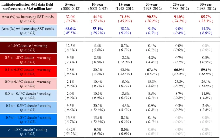
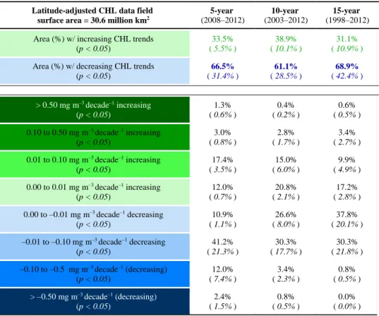
For both datasets, the global datafields were calculated into 0.5° × 0.5° latitude–longitude grids of mean monthly values by year. This process created a global coverage set of nearly 160 000 individual time series, which were then run through the standard IGMETS analysis to calculate trends for each 0.5° box and IGMETS time-window. The OISST, with temperature data from 1982 to present, qualified for all six IGMETS time-windows (TW05–TW30), while the OC-CCI, with chlorophyll data for 1998–2013, only qualified for the 15-year and shorter time-windows (TW05–TW15). The spatio-temporal trends obtained from these datasets were used to create the visual background fields (Section 2.4.4) and to calculate the spatial frequency tables (Section 2.4.5) used in the report.

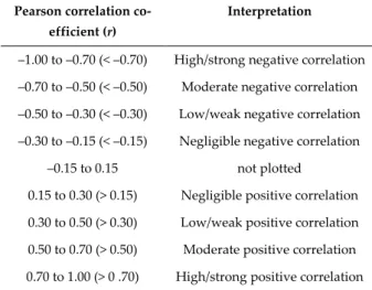
Table 2.2. Summary of correlation strengths based on Pearson correlation coefficient (r) values, modified from Hinkle et al.

(2003).

Pearson correlation co- efficient (r)

Interpretation

–1.00 to –0.70 (< –0.70) High/strong negative correlation –0.70 to –0.50 (< –0.50) Moderate negative correlation –0.50 to –0.30 (< –0.30) Low/weak negative correlation –0.30 to –0.15 (< –0.15) Negligible negative correlation

–0.15 to 0.15 not plotted

0.15 to 0.30 (> 0.15) Negligible positive correlation 0.30 to 0.50 (> 0.30) Low/weak positive correlation 0.50 to 0.70 (> 0.50) Moderate positive correlation 0.70 to 1.00 (> 0 .70) High/strong positive correlation

2.3.4 Correlations with SST and chlorophyll

To detect relationships between in situ variables and sur- face seawater temperatures or chlorophyll concentrations, the Pearson product-moment correlation coefficient was calculated for each in situ variable against its geo- graphically-corresponding, 0.5° × 0.5° satellite-based SST and chlorophyll time series (as discussed in Section 2.3.3).

Satellite data were used, instead of at-site in situ data, in an attempt to create a globally uniform correlation base variable (e.g. not all of the sites had in situ chlorophyll data, and some did not have even in situ temperature data).

The Pearson product-moment correlation is a measure of the strength of a linear association between two variables calculated by trying to draw a best-fit line through these two variables (Hinkle et al., 2002). The Pearson correlation coefficient r indicates how far away these data points are from that best-fit line. This r value indicates the strength of the correlation. Unlike a linear regression, the Pearson product-moment correlation does not declare either variable as dependent or independent and treats all variables equally. Similar to the spatio-temporal trend fields (Sec- tion 2.3.4), spatio-temporal correlation fields were run for each of the 0.5° × 0.5° time-series boxes. Table 2.2 provides interpretations for nine, range-based r value groupings of the Pearson correlation coefficient.

2.4 Visualization of trends

With results from over 340 time series and thousands of variables spanning multiple time-windows, one major challenge IGMETS faced was presenting the results in a way that quickly discerned spatio-temporal trends and patterns within and among variables and regions. This was done by mapping colour-coded symbols that repre- sented in situ trends (Section 2.4.1) and correlations (Sec- tion 2.4.2), creating graphical summary tables (Sec- tion 2.4.3), adding colour-coded backgrounds of spatially complete satellite trends (Section 2.4.4), and summarizing basin-wide statistics of the background field data in a table format (Section 4.5). With thousands of possible variables and time-window configurations, this printed report still only illustrates a small subset of the many different ways to explore the available datasets. For those results not found in this report, the IGMETS Explorer (Sec- tion 2.5) provides an online interface that allows the user to view the full set and variety of all combinations and analyses generated by this first IGMETS analysis.

What are Marine Ecological Time Series telling us about WKH}RFHDQ"

Technical Series 129