Controllability of Time-Aware Processes at Run Time

Controllability of Time-Aware Processes at Run Time

Andreas Lanz¹, Roberto Posenato², Carlo Combi², Manfred Reichert¹

1 Institute of Databases and Information Systems, University of Ulm (Germany)

2 Department of Computer Science, University of Verona (Italy)

Abstract. Companies increasingly adopt process-aware information sys- tems (PAISs) to analyze, coordinate, and monitor their business processes.

Although the proper handling of temporal constraints (e.g., deadlines, minimum time lags between activities) is crucial for many applications, contemporary PAISs lack a sophisticated support of the temporal perspec- tive of business processes. In previous work, we introducedConditional Simple Temporal Networks with Uncertainty (CSTNU)for checking con- trollability of time constraint networks with decision points. In particular, controllability refers to the ability of executing a time constraint network independent of the actual duration of its activities, while satisfying all temporal constraints. In this paper, we demonstrate how CSTNUs can be applied to time-aware business processes in order verify their control- lability at design as well as at run time. In particular, we present an algorithm for ensuring the controllability of time-aware process instances during run time. Overall, proper run-time support of time-aware business processes will broaden the use of PAIS significantly.

Keywords: Process-aware Information System, Temporal Perspective, Temporal Constraints, Process Execution, Controllability

1 Introduction

To stay competitive in their market, companies strive for improved life cycle support of their business processes. In this context, sophisticated IT support for analyzing, modeling, executing, and monitoring business processes becomes crucial [17]. Process-aware information systems (PAISs) offer promising perspec- tives regarding such a process automation. In particular, a PAIS allows defining a business process in terms of an explicitprocess schema, based on whichprocess instances may be created and executed in a controlled and efficient manner [17].

As it has been shown in [12], contemporary PAISs lack a more sophisticated support of the temporal perspective of business processes. However, properly integrating temporal constraints with the design- and run-time components of a PAIS is indispensable to be able to support a greater variety of business processes [3]. Furthermore, in many application domains (e.g., flight planning, patient treatment, and automotive engineering), the proper handling of temporal constraints is crucial for the proper execution and completion of a process [9,4].

instruct procedure

make appointment

inform patient

prepare patient

perform treatment prepare

treatment

Duration maximum 1h

Fixed Date Element appointment Time Lag betw. Activities maximum 2 h

Time Lag betw. Activities minimum 1 h

date

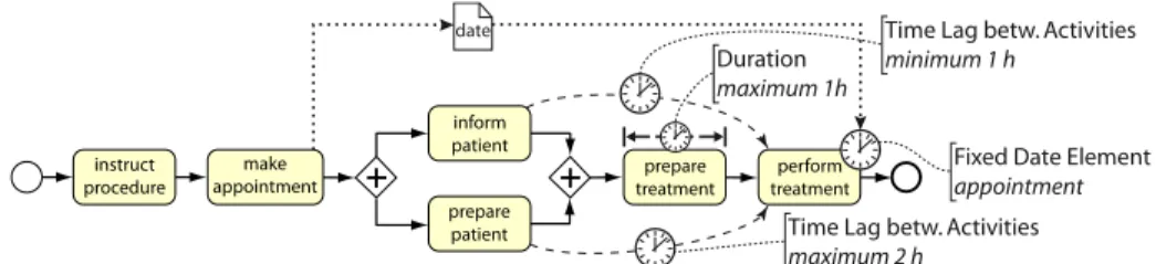
Fig. 1: Illustrating process example with temporal constraints

A fundamental concept related to temporal constraints of process schemas iscontrollability [6]. Controllability is the ability of executing a process schema for all allowed durations of activities and satisfying all temporal constraints. In particular, this ensures that it is possible to execute a process schema without ever having to restrict the duration of an activity to satisfy one of its temporal constraints. Note that this is of paramount importance since activity durations are usually contingent. Indeed, it is possible to set up a duration range for any activity, but the PAIS is aware of the effective duration only after activity completion. Checking controllability is especially important at the presence of alternativeexecution paths (e.g., exclusive choice and loops) as each execution path may lead to different temporal properties of the remaining process.

Checking controllability of a process schema solely at design time, however, is not sufficient. In particular, during the execution of corresponding process instances, temporal constraints need to be continuously updated according to the actual durations of already completed activities as well as the decisions made during run time. Further, note that temporal constraints might not be always known at design time. For example, an appointment with a third party (i.e., the date of a respective activity) is usually made during run time (e.g., in the context of a preceding activity) and is specific for each process instance. As example take the patient treatment process depicted in Fig. 1.³ When considering the temporal perspective of this simplified process, a number of temporal constraints can be observed. In particular, the date for executing activityperform treatment is set by preceding activitymake appointmentand needs to be monitored during run time. In turn, this affects the scheduling of preceding activities due to the other temporal constraints defined, e.g., the patient needs to be preparedat most 2 hours before the actualtreatment takes place. Hence, activityprepare patient needs to be scheduled in accordance with theappointmentof thetreatment.

Obviously, the temporal constraints of this process schema are not very strict, i.e., the temporal perspective of the schema is not over-constrained. Nevertheless, when not meeting these constraints, severe consequences might result. For ex- ample, if the patient is not informedabout the treatmentat least 1 hour before performing thetreatment, the latter must not take place as scheduled for legal reasons and the process has to be aborted. We denote processes obeying a set of defined temporal constraints astime-aware, i.e., the execution of atime-aware

3 Note that we use an extension of BPMN to visualize temporal constraints in processes (cf. Sect. 3 for details).

Category I: Durations and Time Lags TP1 Time Lags between two Activities TP2 Durations

TP3 Time Lags between Events

Category II: Restricting Execution Times

TP4 Fixed Date Elements TP5 Schedule Restricted Elements TP6 Time-based Restrictions TP7 Validity Period Category III: Variability

TP8 Time-dependent Variability

Category IV: Recurrent Process Elements

TP9 Cyclic Elements TP10 Periodicity

Table 1: Process Time Patterns [12]

process is driven by a set of temporal constraints. In particular, for a time- aware process it is necessary to continuously monitor and update its temporal constraints during run time and hence to re-check controllability of the respec- tive process instance. Accordingly, the contribution of this paper is threefold.

First, we discuss fundamental requirements for modeling time-aware processes.

In particular, we provide a basic set of modeling elements required for specifying time-aware processes, as well as for executing corresponding instances during run time. Second, we present a mapping of time-aware process schemas toConditional Simple Temporal Networks with Uncertainty (CSTNU) [5], which allows checking their controllability at build time. Third, we present a sophisticated algorithm that enables flexible controllability checking of time-aware processes during run time as well.

Sect. 2 considers existing proposals relevant in the context of time-aware processes. Sect. 3 provides background information on modeling time-aware processes. In Sect. 4, we show how to check controllability of time-aware processes at both design and run time. Sect. 5 provides a short discussion and evaluation of the proposed approach. Finally, Sect. 6 concludes with a summary and outlook.

2 Related Work

In literature, there exists considerable work on temporal constraints for business processes [10,2,4,13]. However, these approaches focus on design time issues, i.e., issues related to the modeling and verification of time-aware processes. By contrast, run-time support for time-aware processes has been neglected by most approaches so far. The mayor novelty of our work is to explicitly address run-time issues of time-aware processes and to elicit requirements emerging in this context.

In [12], 10 time patterns (TP) are presented, which represent temporal constraints relevant for time-aware processes (cf. Table 1). Further, [11] provides a formal semantics of these time patterns. In particular, time patterns facilitate the comparison of existing approaches based on a universal set of notions with well- defined semantics. Moreover, [11,12] elaborate the need for explicitly considering run-time support for time patterns and time-aware processes, respectively.

Marjanovic et al. [13] define a conceptual model for temporal constraints on a process schema. When taking the time patterns as benchmark, [13] considers time lags between activities (TP1), activity and process durations (TP2), and fixed date elements(TP4). Further, a set of rules for verifying time-aware process schemas is presented. However, no run-time support is considered.

Eder et al. [10] use Timed Workflow Graphs (TWG) to represent temporal properties of activities and their control flow relations. [10] considerstime lags between activities (TP1), activitydurations (TP2),fixed date elements (TP4), andschedule restricted elements (TP5). Further, activity durations are assumed to be deterministic, i.e., be the same for all process instances. In [9], same authors suggest a basic run-time support for time-aware processes assuming that the value of a fixed date element is known when creating the process instance, i.e., setting the particular date during run time is not considered. Based on this,

“internal deadlines” are calculated for each activity making use of the available temporal information.

Bettini et al. [2] suggest an approach quite different from the above ones.

As basic formalismSimple Temporal Network (STN) [8] are used. In an STN, nodes represent time points, while each directed edge a −→^v b between time pointsaandbrepresents a temporal constraintb−a≤v, wherev is a real value.

Note that ifv≥0 holds, the constraint represents the maximum allowed delay betweenb anda; if v <0 holds, it represents the minimum time span elapsed afterabefore the occurrence ofb. Regarding the approach suggested by [2], each activity is represented by two nodes in an STN; i.e., its starting and ending time point. In turn, the edges of the STN represent temporal constraints and precedence relations between the corresponding nodes. [2] considers time lags between activities(TP1), activitydurations(TP2), andfixed date elements(TP4).

However, run-time support of time-aware processes is not considered.

Combi et al. [4] propose a temporal conceptual model for specifying time- aware process schemas. In particular,time lags between activities (TP1), activity durations (TP2),fixed date elements (TP4),schedule restricted elements(TP5), andperiodicity (TP10) are considered. Additionally, [4] discusses how to check consistency of time-aware processes at design time and argues that different strategies for ensuring consistency of a process instance during run time may be applied, depending on the current kind of consistency of a process schema.

The concept of controllability has been mainly investigated in the AI area in connection with temporal constraint networks: [15] proposes an extension of the STN [8], theSimple Temporal Network With Uncertainty (STNU), where the constraints are divided into two classes, the contingent links(not under the control of the system) andrequirement links. In [6], Combi et al. transferred the concept of controllability to time-aware process schemas. In the latter context, informally, controllability is the capability of executing a process schema for all possible durations of all activities and satisfying all temporal constraints.

Recently, [5] extended STNU to Conditional Simple Temporal Network with Uncertainty(CSTNU) that additionally consider alternative execution paths.

3 Modeling Time-Aware Processes

This section provides basic notions needed for understanding this paper. It further defines a basic set of elements for modeling time-aware processes, which allow for a flexible execution of respective process schemas.

3.1 Process Schema

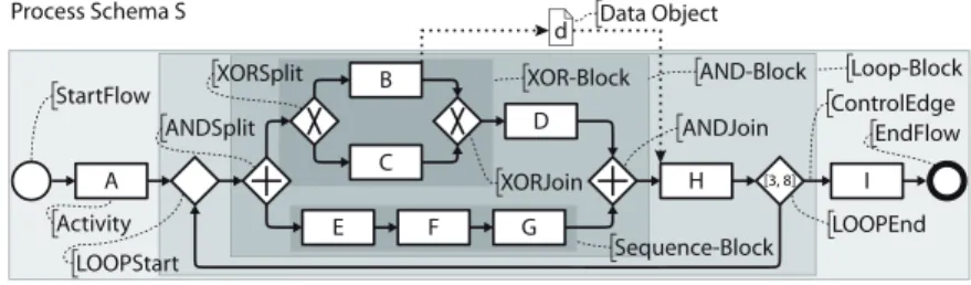
For each business process to be supported, a process schemaneeds to be defined (cf. Fig. 2). In this work, a process schema corresponds to a directed graph, which comprises a set ofnodes – representingactivities andcontrol connectors (e.g., Start-/End-nodes, XOR-splits, or AND-joins) – and a set ofcontrol edges linking these nodes and specifying precedence relations between them as well as loop backward relations. We assume that a process schema is well-structured, i.e., sequences, branchings (i.e., parallel and exclusive choices), and loops are specified in terms of blocks with unique start and end nodes of same type. These blocks—also known as SESE regions [19]—may be arbitrarily nested, but must not overlap; i.e., their nesting must be regular [16]. Fig. 2 depicts an example of a well- structured process schema with the grey areas indicating corresponding blocks.

Each process schema contains a unique start and end node and may be composed of the following control flow patterns [1] (cf. Fig. 2): sequence, parallel split (AND-split), synchronization (AND-join), exclusive choice (XOR-split), simple merge (XOR-join), and structured loops. Note that these patterns constitute the core of any process meta model and allow for the flexible composition of more complex structures [14]; further, they cover most processes found in practice [14].

We further assume that the start and the end nodes of a structured loop are distinct from normal XOR-join and XOR-split nodes, i.e., there is an explicit loop construct in the process meta model (like in ADEPT [7]).⁴ Finally, to be able to reason about the temporal properties of a loop and to ensure termination of any process schema execution, each loop-end node is augmented with a minimum and maximum number of possible iterations of the respective loop. Note that this does not pose an actual restriction as it is always possible to find a maximum number of iterations high enough to cover any possible case.

In addition to the described control flow elements, a process schema contains process-relevantdata objects as well asdata edges linking activities with data objects. More precisely, a data edge either represents a read or write access of the referenced activity to the referred data object.

Process activities may either beatomic orcomplex. While anatomic activity is associated with an application service, a complex activity refers to asub-process.

In our work, we consider complex activities as self-contained, i.e., there is no direct relation between a sub-process and the respective parent process. Therefore, we do not differentiate between atomic and complex activities.

Even though we mostly use the notation defined by BPMN for illustration purpose, the approach described in the following is not specific to BPMN. To set a focus we restrict ourselves to a set of basic modeling elements found in almost every process meta model. Furthermore, to graphically distinguish between loop-blocks and XOR-blocks we use the exclusive gateway symbol with an “X”

to represent an XOR-split/-join and the symbol without an “X” to represent loop-start and loop-end nodes.

4 Note that this does not apply to BPMN causing additional complexity when analyzing processes.

A

B

D C

E F

I G

H ^{[3, 8]}

XORJoin

ANDJoin

Activity LOOPStart

ControlEdge

LOOPEnd StartFlow

ANDSplit XORSplit

EndFlow Process Schema S

Loop-Block AND-Block

XOR-Block

Sequence-Block d Data Object

Fig. 2: Core Concepts of a Process Meta Model

At run time,process instances are created and executed according to the defined process schema. In turn, activity instancesrepresent executions of single process steps (i.e., activities) of such a process instance. If a process schema contains one or more XOR- or LOOP-blocks, not all process instances perform exactly the same set of activities. The concept ofexecution pathallows identifying which activities and control connectors are performed during an execution.

Given a process schema P, an execution path p (exe-path) denotes a connected maximal subgraph of the process schema containing its Start- and End-nodes, in which all XOR-split connectors have exactly one branch and each loop block has a fixed number of repetitions. In particular, each execution path represents one possible execution of the respective process schema. In turn, the set of all exe-paths of process schemaP is denoted asExePaths_P. Anexe-path p can be also briefly described by a string containing the activity identifiers of the exe-pathsorted w.r.t. their execution order and separated by a dash if the order is sequential or by a vertical bar if it is parallel [4]. Considering the schema from Fig. 2, the string A-((B-D)|(E-F-G))-H-Irepresents an example of anexe-path, whereAis followed by a parallel execution of two sequential paths (B-D) (i.e., for the XOR-split the upper path is selected) and (E-F-G); then,Hand Iare sequentially executed. Note that setExePathsP may have an exponential cardinality w.r.t. the number of XOR- or LOOP-blocks in the schema.

3.2 Time-aware Process Schemas

Regarding the time patterns (TP) presented in Sect. 2, to set a focus, this work specifically considers the ones most relevant in practice [12]; i.e.,time lags between two activities(TP1),durations (TP2) of activities,fixed date elements (TP4) of activities, andcyclic elements(TP9).

Anactivity duration(TP2) represents the time span allowed for executing an activity (or node, in general), i.e., the time span between start and completion of the activity [12]. We assume that each activity of a process schema has an assigned duration. Usually, activity durations are described in terms of minimum and maximum values. Even though these values are known for an activity at design time, the actual duration of a corresponding activity instance is only known at run time after its completion (i.e., it is contingent). Consequently, activity durations must not be restricted when checking controllability at design or run time to satisfy all temporal constraints specified on a process schema. However,

in reality, in most cases activity durations are either based on the experience of a domain expert or extracted from process logs. Therefore, activity durations usually represent worst case estimates, i.e., respective maximum durations often cover cases with an exceptionally long duration. Further, execution times of most activities can be shortened if necessary. Accordingly, activity durations may be restricted to some extend during design time when verifying controllability or during run time. In particular, an activity has aflexible maximum duration M axDF. If necessary this may be restricted up to a contingentminimum and maximum duration range [M inDC, M axDC], which, in turn, must be at least available to the agent when executing the activity. Therefore, activity durations are expressed in terms of restrictable time intervals [[M inDC, M axDC]M axDF]G where 1≤M inDC ≤M axDC≤M axDF5 andGcorresponds to the time unit used (i.e., temporal granularity like minutes, hours,. . . ).⁶If a flexible maximum duration is not applicable for an activity, we write [[M inD_C, M axD_C]]G for short. If a process designer does not set a duration for an activity [[1,1]∞]M inG is used as default value, where M inGcorresponds to the minimum time unit used by the system. Since control connectors are automatically executed by the PAIS and solely serve structuring purposes, we assume that they have a fixed duration defined by the PAIS (e.g., [[1,1]]M inG) that cannot be modified by the process designer.

Time lags between two activities(TP1) restrict the time span allowed between the starting/ending instants of two activities [12]. Such a time lag may not only be defined between directly succeeding activities, but between any two activities that may be conjointly executed in the context of a particular process instance, i.e., the activities must not belong to exclusive branches. A time lag is visualized by a dashed edge with a clock between the source and target activity (cf. Fig. 3). The label of the edge specifies the constraint according to the following template: hISi[M inD, M axD]GhITi; thereby, hISi ∈ {S, E}and hITi ∈ {S, E} mark the instant (i.e., starting/ending) of the source and target activity the time lag applies to; e.g., hISi = S marks the starting instant of the source activity andhITi=E the ending instant of the target activity. In turn, the interval [M inD, M axD]Grepresents the range allowed for the time span between instants hISi and hITi using time unit G. Further, we assume that−∞ ≤M inD≤M axD≤ ∞holds. In particular, time lags may be used to specify minimum delays and maximum waiting times between succeeding activities. As example consider the time lagE[5,60]min S betweenEandFin Fig. 3. It expresses that there is an end-start time lag (hISi=E, hITi=S) of [5,60]minbetween the two activities; i.e., the delay between the end of Cand the start of F must be at least 5 minutes, while the waiting time between the two must be at most 60 minutes. Finally, it is noteworthy that there exists an

5 0 as minimum value for a duration is disallowed since it is not possible to execute an activity/control connector without consuming time.

6 For the sake of clarity, we assume that all temporal values are expressed using the same granularity; if different granularities are used, it is required to convert them to a common one before executing the process [4].

implicitE[1,∞]M inG S constraint between any couple of directly succeeding activities, i.e., the second activity may only be started after completing the first.

In extension to time lags between activities,cyclic elements(TP9) allow process designers to restrict the time span between activity instances belonging to different iterations of a loop structure [12]. This may either be instances of a specific activity or two different activities of the same loop structure. Like time lags, a cyclic element is visualized as dashed edge (with a clock) between the two activities. To differentiate between the two, the label of a cyclic element is extended by a “^∗” next to the allowed range: hISi[M inD, M axD]G^∗hITi. For the sake of simplicity, we only consider cyclic elements between two directly succeeding iterations. However, this is no restriction of the presented algorithms and may be easily extended if necessary.

Finally,fixed-date elements(TP4) for activities allow restricting the execu- tion of an activity in relation to a particular date [12],⁷e.g., a fixed-date element may define that the activity must not be started before or must be completed by a particular date. Generally, the value of a fixed-date element is specific to a process instance, i.e., it is not known before creating the process instance or even becomes known only during run time. Therefore, the particular date of a fixed-date element is part of process-relevant data, i.e., it is stored in a data object during run time. When evaluating the fixed-date element, the respective data object is accessed and its current value is retrieved [11]. Graphically, a fixed-date element is visualized by a clock symbol attached to the respective activity (cf.

Fig. 3). The labelhDi ∈ {E_S, L_S, E_E, L_E} attached to this clock corresponds to the activity’s earliest start date (ES), latest start date (LS), earliest completion date (EE), or latest completion date (LE), respectively.

As an example, Fig. 3 shows a process schema exhibiting several temporal constraints. Though some of the symbols used for visualizing the temporal constraints resemble timer events from BPMN, their semantics is quite different and should not be mixed up. ActivitiesA,E,F, andH have an activity duration attached. The one of A, for example, expresses thatAhas a flexible maximum duration of 25min. This may be further restricted to a contingent minimum duration of 5minand a maximum duration of 20minif necessary. In turn, the activity duration of H expresses that H has a contingent minimum duration of 60minand a maximum duration of 120min, which must not be restricted any further. Between BandGthere is a time lag described byS[30,120]min S.

Additionally, there is a time lag betweenEand F. Note that, in case a time lag restricts the time span between two directly succeeding activities, for the sake of readability, we attach the clock directly to the control edge and omit the dashed edge of the time lag. However, this is only a graphical simplification and does not change semantics. Next, there is a cyclic element S[0,120]min^∗S between BandF. It describes that between the start of any instance of Band the start of an instance of Fin the succeeding iteration, there is a time span of at most 120min. Finally, Ghas a fixed-date element attached to it, whereby label LE 7 Fixed-date elements are often referred to as “deadlines”. However, this does not

completely meet the intended semantics.

A

B

D C

E

H F

G ^{[3, 8][3, 8]}

[[5, 20] 25]min

[[5, 35] 40]min [[10, 20] 25]min

[[60, 120]]min L_E

S [0, 120]min* S S [30, 120]min S

d

E [5, 60]min S

Cyclic Element Process Schema S

Fixed Date Element

Activity Duration

Date value for Fixed Date Element G Time Lag between two Activities

Time Lag between two Activities Fig. 3: Process with Temporal Constraints

indicates that the latest end date of the activity is restricted by the temporal constraint. In turn, the date of the fixed-date element is provided by activityD through data object d. Particularly, for each iteration of the loop, a new value for the fixed-date element of Gis provided by D.

4 Executing Time-Aware Processes

This section introduces and discusses the concept ofcontrollabilityof a time-aware process schema. Controllability guarantees that a process schema can be correctly executed considering all temporal constraints. More specifically, we first introduce the concept of controllability and the controllability check problem. Then, we show how to deal with the execution of a controllable time-aware process schema.

4.1 Controllability of Time-Aware Process Schemas

In general, controllability corresponds to the capability of a PAIS to execute a process schema for all possible contingent durations of all activities while still satisfying all temporal constraints; i.e., controllability ensures that it is possible to execute a process schema without ever having to restrict the contingent duration of an activity to satisfy one of the other temporal constraints.

In particular, anexe-path(cf. Sect. 3.1) is executed by performing activities and control connectors, thereby observing any structural and temporal constraints of the process schema. We denote a process schema ascontrollableif it is possible to perform anyexe-pathsatisfying all temporal constraints without restricting contingent activity durations involved in the exe-path. If there are no time lags (TP1), or fixed date elements (TP4) the schema is controllable. Otherwise, it is necessary to verify and, possibly, adjust time lags in order to guarantee controllability of the process schema.

In [5], authors proposedConditional Simple Temporal Network with Uncer- tainty (CSTNU) to represent and analyze a network of temporal constraints, where some constraints hold according to specific run-time-evaluated data condi- tions. Furthermore, they presented a sound algorithm that allows checking the controllability of a CSTNU (possibly adjusting non-contingent constraints) in exponential time w.r.t. the number of conditions in the worst (theoretical) case.

Moreover, they provided an implementation of the algorithm showing that it is possible to manage the conditions in an appropriate way in order to avoid the worst case and obtain a practical fast convergence of the algorithm. In this paper, we propose to use the CSTNU checking algorithm to verify the controllability of a process schema extended with the temporal aspects (as discussed in Sect. 3.2). We propose to use CSTNU for two reasons: 1) it is preferable to exploit checking and execution algorithms for a well founded model of extended temporal constraint representation instead of developing new native algorithms, and 2) all other models for temporal constraint representation in literature (e.g., [15,18]) do not allow an effective representation and management of conditional executions with uncertainties.

We now show how to use CSTNU to check the controllability of the considered time-aware process schema (cf. Sect. 3) at design time as well as run time. In particular, a CSTNU is an STN extended with the following constructs:

– observation nodes: each observation node is associated with a specific proposi- tion (cf. node E associated with propositionP in Fig. 5-b). The truth-value of the proposition is determined when the node is executed. Informally, an ob- servation node represents the time point at which a relevant information (i.e., proposition) for the execution of the CSTNU is acquired, i.e., it represents the time point a decision is made.

– labeled nodes and edges: nodes and edges are characterized by a label con- sisting of propositions. Such nodes and labels are considered only when the corresponding propositions hold (cf. edge labelsβ,P β and¬P βin Fig. 5-b).

Informally, during an execution, the system maintains the truth values of propositions as the executionscenario. Then, it considers only nodes and edges having a label consistent with the scenario.

– contingent links: a contingent link represents an uncontrollable-but-bounded temporal interval. Each contingent link is described by the range [x, y], 0< x < y <∞, between two time-point variables (nodes),AandC, where Cis the so calledcontingenttime point. OnceAis executed,Cis guaranteed to execute such thatC−A∈[x, y]. However, the particular time at whichC executes is uncontrollable.

In the CSTNU model, each edge has alabeled valuedescribing the meaning of the corresponding constraint. Alabeled valueis a triplehPLabel, ALabel, Numi where:

– PLabel is a propositional label representing a conjunction of propositions.

Usually,α, β, . . .are used for representing conjunctions of propositions.

represents an empty label.

– ALabel is an alphabetic label, and either is:

• an upper-case letter,C, specifying the upper bound of a contingent link;

• a lower-case letter,c, specifying the lower bound of a contingent link; or

• , representing no alphabetic label, representing an ordinary STN edge.

– Num is a real number, representing the value of the constraint.

A [[xC, yC]yF]

(a)

AS AC AE

hβ,,∞i

hβ,,−1i

hβ,,∞i

hβ,,−1i hβ, ac, xCi

hβ, A_C,−y_Ci

hβ,, yF−xCi hβ,, yFi

hβ,,0i

(b)

Fig. 4: (a) An activity with a duration. (b) CSTNU translation.

A possible technique to translate a process schema into an equivalent CSTNU consists of mapping each process construct into an equivalent (with respect to the temporal constraints) CSTNU fragment.

More formally,

Theorem 1. Given a time-aware process schemaP_S, there exists a correspond- ing CSTNU N such that all temporal features ofP_S are represented in N. Proof. The proof is given by construction. In the following, we will provide the mapping for the time-aware process constructs, discussing the most important mappings from the point of view of the temporal behaviour.

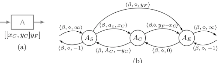
First the Start-/End-nodes of the process schema are mapped to two nodes, Z and W, respectively. In turn, an activity and its incoming/outgoing edges are mapped to CSTNU as shown in Fig. 4. In particular, each activityAwith duration [[xC, yC]yF] corresponds to three nodesAS,AC, andAE, which represent the starting time-point, contingent ending time-point, and ending time-point, respectively, linked by appropriate edges representing the give duration. The contingent ending time-point AC is the uncontrollable ending point bounded by the contingent range [xC, yC] with respect to the starting time-point AS. The ending time-pointAE is the controllable ending point that allows the run- time algorithm to consider the flexible maximum durationyF, represented by a upper-bound constraint between AS and AE with Plabel hβ,, yFi. Edges betweenA_S andA_C represent contingent links in CSTNU; edges between A_C andA_E represent ordinary constraints; finally, any incoming (outgoing) edge of the activity is translated as a pair of edges representing the implicit temporal constraint [1,∞] between the ending (starting) node of the predecessor (successor) activity and the starting (ending) node of the considered activity.

The next construct to be considered is the XOR-split. Fig. 5 depicts the translation of an XOR-split evaluating a propositionP. The connector corre- sponds to two nodes, S and E, representing its starting and ending instants, respectively. These nodes are connected by two edges representing the implicit duration range [1,1]. _Eis theobservation node for propositionP. All edges and nodes corresponding to activities, connectors and control edges in the XOR-block are suitably labeled withP or¬P depending on the branch they belong to. The corresponding XOR-Join is translated in a similar way, but the outgoing edge then corresponds to two edges in which propositionsP/¬P are not present (cf.

Fig. 6).

P?

true

false

(a)

S ^E

P?

hβ,,∞i

hβ,,−1i

hβ,,1i

hβ,,−1i

hP β,,∞i

hP β,,−1i

h¬P β,,∞i

h¬P β,,−1i

(b)

Fig. 5: (a) XOR-split with implicit duration [1,1]. (b) CSTNU translation.

(a)

S E

hβ,,∞i

hβ,,−1i hβ,,1i

hβ,,−1i hP β,,∞i

hP β,,−1i h¬P β,,−1i

h¬P β,,∞i

(b)

Fig. 6: (a) XOR-Join with implicit duration [1,1]. (b) CSTNU translation.

(a)

AE

AS hβ,,1i hβ,,−1i

w1 w2

hβ,,0i hβ,,0i hβ,, t1i hβ,, t2i hβ,,∞i

hβ,,−1i

hβ,,∞i

hβ,,−1i

hβ,,∞i hβ,,−1i

(b)

Fig. 7: (a) AND-Join connector. (b) CSTNU translation.

Another construct to be considered is the AND-Join connector (the mapping of the AND-Split connector is straightforward). Fig. 7-(a) depicts an example of an AND-Join connector with two incoming flows. The execution of this connector requires waiting for all incoming flows: after the last incoming flow has been triggered, the AND-Join is executed before triggering its outgoing edge. The key aspect of the AND-Join is that its incoming flows may arrive at different instants. Therefore, each incoming flow is connected to a “wait” node that, in turn, is connected toAS by two edges, as depicted in Fig. 7-(b). For example, the constrainthβ,,0icorresponding to edge (AS, w1) represents that AS must be afterw1, while the constrainthβ,, t1ion edge (w1, AS) represents the possible maximum delay due to the execution ofw2; the valuet1 is automatically determined by the controllability check at design time. One can easily show that if there are more incoming flows in the original AND-Join connector, it is possible to translate it using a sequence of pairs of “wait” nodes properly connected beforeA_S.

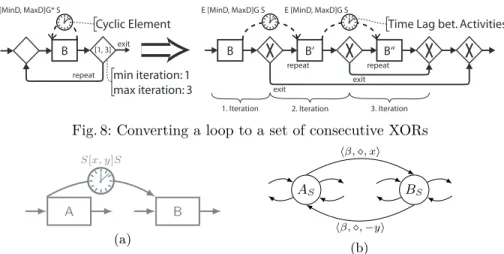
Since for each loop the maximum number of iterations is known, any process schema containing loops can be rewritten into a loop-free one. For this, the loop

B

min iteration: 1 max iteration: 3

repeat [1, 3] exit

Cyclic Element Time Lag bet. Activities

B B‘ B‘‘

repeat repeat

exit exit

1. Iteration 2. Iteration 3. Iteration

E [MinD, MaxD]G* S E [MinD, MaxD]G S E [MinD, MaxD]G S

Fig. 8: Converting a loop to a set of consecutive XORs

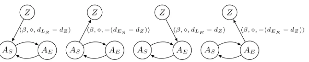
A B

S[x, y]S

(a)

AS BS

hβ,, xi

hβ,,−yi

(b)

Fig. 9: (a) Start-start time lag between activitiesAandB. (b) CSTNU translation.

block is replaced by a block containing clones of the original loop body, which are then linearly connected: all Loop-start connectors are removed and each Loop-end connector becomes an XOR-split connector with one edge connected to the first node of the following clone and the other connected to an XOR- join connector inserted after the last clone. The condition of these XOR-split connectors corresponds to the original condition of the Loop-end connector.

Moreover, cyclic elements (TP9) are transformed to time lags (TP1) between the clones of respective activities. Fig. 8 shows an example of such an unfolding of a loop with at maximum three iterations. Consequently, a loop may be translated to CSTNU the same way as XOR-splits and -joins (cf. Figs. 5 and 6).

Next, a time lag between two activities (TP1) can be translated into a pair of CSTNU edges between between the starting/ending nodes of the two activities. In particular, for each time laghISi[x, y]GhITi, depending on the value ofhISi/hITi, a pair of ordinary constraint edgeshβ,, xiandhβ,,−yiis added between the starting/ending node of the source and the starting/ending node of the target activity. Fig. 9 depicts this transformation exemplarily for a start-start time lag (i.e.,hISi=S andhITi=S).

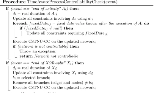
The last major construct we consider for the translation is the fixed date constraint (TP4). It can be translated into a CSTNU edge between the start nodeZ of the process and the node representing the starting/ending node of the activity once the starting timed_Z of the process and the fixed dated_hDi value are known, i.e., the fixed date is represented as the time lag between the start of the process instance and the respective fixed date. Fig. 10 depicts the details of the translation of the different fixed date elements according to the constraint labelhDi ∈ {ES, LS, EE, LE}. This completes the proof. ut 4.2 Run-Time Controllability Check

Controllability of a process schema must be checked both at design and run time. At design time, such a controllability check allows guaranteeing that the

Z

AS AE hβ,, d_LS−dZi

Z

AS AE hβ,,−(d_ES−dZ)i

Z

AS AE

hβ,, d_LE−dZi

Z

AS AE

hβ,,−(d_EE−dZ)i

Fig. 10: Translating possible fixed date constraints on an activity Awhen date dZ of the process start and datedE_S|dL_S|dE_E|dL_E of the constraint are known.

design phase is sound as any process instance may be executed meeting the given temporal constraints. At run time, the controllability check updates the temporal network according to the real durations of already executed activities, to the possible fixed date constraints, and to the current execution path. In particular, controllability has to be checked after the completion of each contingent activity.

When creating a process instance, a copy of the CSTNU created at design time is made. Next, any fixed date constraint known at process creation time is considered by adding the respective constraint(s) (cf. Sect. 4.1). This CSTNU is then updated according to the starting time of the process instance by execut- ing a controllability check. Thus, the time frame for starting the first activity, determined by the previous check, is fixed and is used by the execution engine.

When completing an activity, its real duration and possible date value for fixed date constraints become known. Hence, in order to maintain the right time frames of unexecuted activities, it is necessary to update and check the CSTNU after the completion of each activity. In particular, the check may result in an update of the time frames of the remaining activities. Then, the engine determines the following activities to execute, taking into account the order given by the schema and the time frames provided by the updated CSTNU. Note that there are different possible execution strategies for choosing the exact instant to start an activity within its time frame. In the following we presume an execution strategy that allows executing an activity/connector as soon as it becomesenabled. An activity/connector is enabled when all its previous activities/connectors (w.r.t. the process schema) have been executed and all constraints involving the considered activity/connector are met. However, if—due to some delay—an activity is not started within its time frame or if it takes longer than permitted by the CSTNU, the process instance (potentially) becomes uncontrollable (i.e., it can no longer be guaranteed that the process may be completed without violating any time constraint). In this case, time-specific exception handling (i.e., escalations) should be triggered [9].

Let us label the CSTNU controllability checking algorithm as CSTNU-CC.

For a process instance, the check of its controllability during run time, which we call TimeAwareProcessControllabilityCheck, works as follows:

1. Once the starting time of a process instance is set, all fixed date constraints whose date is also known at process creation time are translated into equivalent constraints w.r.t. to the starting date of the process instance (cf. Fig. 10) in the CSTNU instance. The controllability of the CSTNU instance is then checked

to ensure that any fixed date constraint is consistent with the execution time of the process instances.

2. Each time an activity is completed, the CSTNU instance is updated using the real duration of the completed activity and re-checked to propagate the modified constraints.

3. After the completion of any activity producing a date value for a fixed-date constraint, the CSTNU instance must be updated adding the equivalent constraint(s) as shown in the previous section (cf. Fig. 10) and then re- checked. For networks being controllable at design time it is noteworthy that, besides activity executions not being started within the time frames given by the CSTNU or not respecting the given activity duration constraint, only fixed date constraints could make the network uncontrollable at run time.

4. Each time an XOR-split is completed, the CSTNU instance must be updated by removing all nodes and edges belonging to skipped XOR branches. In particular, the execution of an XOR-split determines the one of the corre- sponding observation node. Such observation node determines the truth value of the associated proposition. Therefore, the executionscenario is updated and all nodes/edges not consistent with it are removed. Note that, due to the removal of the skipped XOR branches, the time frames of unexecuted activities may be potentially relaxed.

Fig. 11 depicts the pseudocode of algorithmTimeAwareProcessControllability- Check. It checks the controllability of the corresponding CSTNU network during

run time according to the above approach.

Let us consider in a more detailed way how many timesTimeAwareProcess- ControllabilityCheck is executed for a process instance. Letk be the number of XOR-split connectors andathe number of activities.TimeAwareProcessControl- labilityCheck is then calledk+atimes in the worst case (sequential XOR-splits containing activities in only one branch each). EachTimeAwareProcessControl- labilityCheck execution corresponds to a single execution of the CSTNU-CC algorithm. The latter has an exponential-time complexity w.r.t. to the numberk⁰ of unexecuted XOR-splits, wherek⁰ =k, k−1, . . . ,1. Each unexecuted XOR-split determines at least 2 different outgoing execution paths and, thus, there exist at least 2^k0 different possible execution paths in the process instance. Sincek decreases linearly during the execution (worst case), the complexity of the follow- ing CSTNU-CC executions—after each XOR-split—decreases exponentially. As for the CSTNU-CC algorithm [5], the real time complexity of the controllability check algorithm is much lower than the theoretical worst case. First experiments we performed have confirmed this.

5 Discussion

Recently, we identified a set of time patterns for evaluating the support of the temporal perspective in PAIS [12,11]. Empirical evidence we gained in case studies has confirmed that these time patterns are common in practice and required for properly modeling the temporal perspective of processes in a variety of

Procedure TimeAwareProcessControllabilityCheck(event) if (event == “end of activity”Ai)then

di= real duration ofAi;

Update all constraints involvingAiusingdi;

foreachf ixedDateij=fixed date value known after the execution of Aido if (f ixedDateij6=null)then

Update all constraints requiringf ixedDateij; Execute CSTNU-CC on the updated network;

if (network is not controllable)then Throw an exception;

returnNetwork not controllable if (event == “end of XOR-split”Xi)then

di= real duration ofXi;

Update all constraints involvingXiusingdi; bi= selected branch;

Remove all branches (edges and nodes)6=bi; Execute CSTNU-CC on the updated network;

returnNetwork controllable;

Fig. 11: Pseudo code for controllability checking of time-aware processes during run time

domains [12]. In particular, our case studies revealed the need for a comprehensive design- and run-time support of time-aware process. This has been confirmed in a number of discussions, we had with process engineers when validating the formal semantics of our time patterns [11].

To ensure the soundness of a process schema and hence robust and correct execution of corresponding process instances, the controllability of their temporal constraints must be checked. In general, to solely verify time-aware process schemas at design time is neither sufficient nor completely possible. Recent work has shown that certain time patterns (i.e., temporal constraints) cannot be verified at design time, as they are specific for each process instance [12].

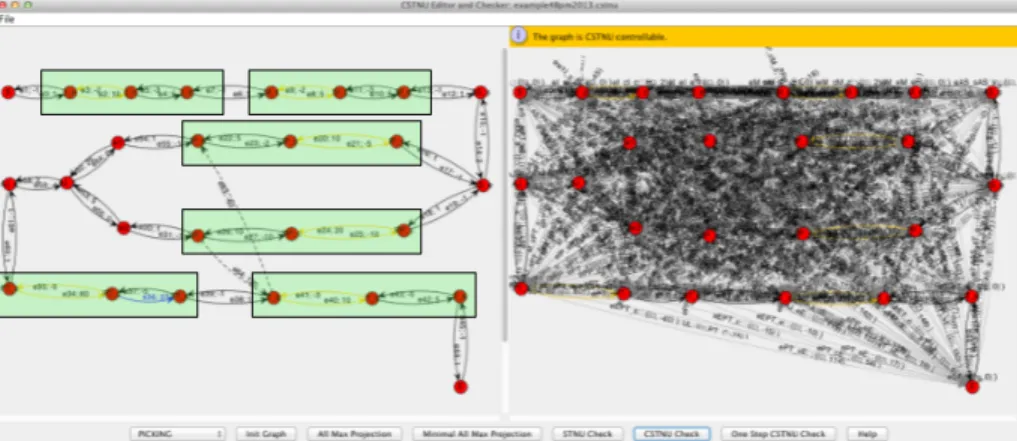
The time patterns considered in this paper were selected based on the empirical evaluation we conducted as part of [12]. In particular, they are the ones most commonly required in practice. Also, note that the particular patterns provide a reference time frame for any instance based on respective time-aware process schemas. To verify and test the practical usability of the proposed transformation and respective algorithms, we implemented a proof-of-concept prototype as part of CSTNUEditor[5]. It allows us to create a CSTNU instance based on a process schema and to check its controllability. First tests have shown that the algorithm finds the solution in an average number of iterations one order of magnitude smaller than the theoretical estimated upper bound. As an example, Fig. 12 depicts the CSTNUEditor screenshot of the controllability check of the process schema of Fig. 1: the left part of the screen shows the CSTNU corresponding to the process schema (green boxes contain nodes and constraints corresponding

Fig. 12: Time-aware Process controllability check in CSTNUEditor to original activities), while the right part depicts all the computed temporal constraints between nodes together with the overall analysis result showing that the process is controllable. Moreover, we have implemented most of the time patterns as part of a proof-of-concept prototype based on the AristaFlow BPM Suite [7]. In this context, we are working on integrating the presented algorithms for controllability checking at build time and during run time to obtain atime- and process-aware information system.

6 Summary and Outlook

Time is a fundamental concept regarding the support of business processes. In a real world environment, where even small delays may cause significant problems, it will be crucial for any enterprise to be aware of the temporal constraints of its business processes as well as to control and monitor them during process execution.

Particularly, it must be ensured that no temporal constraint is violated during run time. This paper considered fundamental requirements for the run-time support of time-aware processes.

First, we defined a set of basic elements for modeling time-aware process schemas, which allow for a flexible execution of related processes instances.

Specifically, we considered the need for dynamically adapting process instances to a specific context, e.g., we consider temporal constraints whose parameters only become known during process execution. The proposed set of temporal constraints is independent from a particular process modeling language.

Second, we presented a transformation of time-aware process schemas toCon- ditional Simple Temporal Networks with Uncertainty for checking controllability of respective process schemas at design time. We then demonstrated how this can be also applied for ensuring the controllability of corresponding time-aware process instances during run time. In particular, we presented an algorithm for controllability checking during run time and discussed its complexity.

In future work, we will investigate the complexity of the presented controlla- bility checking algorithm in more detail. In this context, we will examine how

process abstractions and process views as well as predictive knowledge about XOR decisions may be applied to reduce the complexity of this algorithm. Fur- thermore, we will fully integrate the presented approach with the AristaFlow BPM Suite [7]. Finally, we will evaluate the impact, process changes have on time-aware processes and respective temporal constraints.

References

1. van der Aalst, W.M.P., ter Hofstede, A.H.M., Kiepuszewski, B., Barros, A.P.:

Workflow patterns. Distributed and Parallel Databases 14(1), 5–51 (2003) 2. Bettini, C., Wang, X.S., Jajodia, S.: Temporal reasoning in workflow systems.

Distributed and Parallel Databases 11(3), 269–306 (2002)

3. Combi, C., Gozzi, M., Juarez, J.M., Oliboni, B., Pozzi, G.: Conceptual modeling of temporal clinical workflows. In: Proc. TIME’07. pp. 70–81. IEEE (2007)

4. Combi, C., Gozzi, M., Posenato, R., Pozzi, G.: Conceptual modeling of flexible temporal workflows. ACM Trans. Auton. Adapt. Syst. 7(2), 19:1–19:29 (Jul 2012) 5. Combi, C., Hunsberger, L., Posenato, R.: An algorithm for checking the dynamic controllability of a conditional simple temporal network with uncertainty. In: Proc.

Int. Conf. Agents & Art. Int. (ICAART). vol. 2, pp. 144–156. SciTePress (2013) 6. Combi, C., Posenato, R.: Controllability in temporal conceptual workflow schemata.

In: BPM’09. pp. 64–79. Springer (2009)

7. Dadam, P., Reichert, M.: The ADEPT project: A decade of research and devel- opment for robust and flexible process support - challenges and achievements.

Computer Science - R&D 22(2), 81–97 (2009)

8. Dechter, R., Meiri, I., Pearl, J.: Temporal constraint networks. Artif. Intell. 49(1-3), 61–95 (1991)

9. Eder, J., Euthimios, P., Pozewaunig, H., Rabinovich, M.: Time management in workflow systems. In: Proc. BIS’99. pp. 265–280. Springer (1999)

10. Eder, J., Gruber, W., Panagos, E.: Temporal modeling of workflows with conditional execution paths. In: Proc. DEXA’00. pp. 243–253. Springer (Sep 2000)

11. Lanz, A., Reichert, M., Weber, B.: A formal semantics of time patterns for process- aware information systems. Tech. Rep. UIB-2013-02, University of Ulm (2013) 12. Lanz, A., Weber, B., Reichert, M.: Time patterns for process-aware information

systems. Requirements Engineering (2012)

13. Marjanovic, O., Orlowska, M.E.: On modeling and verification of temporal con- straints in production workflows. Knowl. and Inf. Syst. 1(2), 157–192 (1999) 14. Mendling, J.: Metrics for process models: empirical foundations of verification, error

prediction, and guidelines for correctness. Springer (2009)

15. Morris, P.H., Muscettola, N., Vidal, T.: Dynamic control of plans with temporal uncertainty. In: IJCAI. pp. 494–502 (2001)

16. Reichert, M., Rinderle, S., Kreher, U., Dadam, P.: Adaptive process management with ADEPT2. In: Proc. ICDE’05. pp. 1113–1114. IEEE (2005)

17. Reichert, M., Weber, B.: Enabling Flexibility in Process-aware Information Systems:

Challenges, Methods, Technologies. Springer (2012)

18. Tsamardinos, I., Vidal, T., Pollack, M.E.: CTP: A new constraint-based formalism for conditional, temporal planning. Constraints 8, 365–388 (2003)

19. Vanhatalo, J., Völzer, H., Leymann, F.: Faster and more focused control-flow analysis for business process models through SESE decomposition. In: Proc. ICSOC’07. pp.

43–55. Springer (2007)