Algorithmic transformation of multi-loop Feynman integrals to a canonical basis

(1)

Algorithmic transformation of multi-loop Feynman integrals to a canonical basis

D I S S E R T A T I O N

zur Erlangung des akademischen Grades doctor rerum naturalium

(Dr. rer. nat.) im Fach Physik

Spezialisierung: Theoretische Physik eingereicht an der

Mathematisch-Naturwissenschaftlichen Fakultät der Humboldt-Universität zu Berlin

von

Herrn M.Sc. Christoph Meyer

Präsidentin der Humboldt-Universität zu Berlin:

Prof. Dr.-Ing. Dr. Sabine Kunst

Dekan der Mathematisch-Naturwissenschaftlichen Fakultät:

Prof. Dr. Elmar Kulke Gutachter:

1. Prof. Dr. Peter Uwer 2. Prof. Dr. Dirk Kreimer 3. Prof. Dr. Stefan Weinzierl

Tag der mündlichen Prüfung: 22. Januar 2018

(2)

(3)

Abstract

The evaluation of multi-loop Feynman integrals is one of the main challenges in the computation of precise theoretical predictions for the cross sections measured at the LHC. In recent years, the method of differential equations has proven to be a powerful tool for the computation of Feynman integrals. It has been observed that the differential equation of Feynman integrals can in many instances be transformed into a so-called canonical form, which significantly simplifies its integration in terms of iterated integrals.

The main result of this thesis is an algorithm to compute rational transformations of differential equations of Feynman integrals into a canonical form. Apart from requiring the existence of such a rational transformation, the algorithm needs no further assumptions about the differential equation. In particular, it is applicable to problems depending on multiple kinematic variables and also allows for a rational dependence on the dimensional regulator. First, the transformation law is expanded in the dimensional regulator to derive differential equations for the coefficients of the transformation. Using an ansatz in terms of rational functions, these differential equations are then solved to determine the transformation.

This thesis also presents an implementation of the algorithm in the Mathematica package CANONICA, which is the first publicly available program to compute transformations to a canonical form for differential equations depending on multiple variables. The main functionality and its usage are illustrated with some simple examples. Furthermore, the package is applied to state-of-the-art integral topologies appearing in recent multi-loop calculations. These topologies depend on up to three variables and include previously unknown topologies contributing to higher-order corrections to the cross section of single top-quark production at the LHC.

(4)

(5)

Zusammenfassung

Die Auswertung von Mehrschleifen-Feynman-Integralen ist eine der größ- ten Herausforderungen bei der Berechnung präziser theoretischer Vorher- sagen für die am LHC gemessenen Wirkungsquerschnitte. In den ver- gangenen Jahren hat sich die Nutzung von Differentialgleichungen bei der Berechnung von Feynman-Integralen als sehr erfolgreich erwiesen. Es wurde dabei beobachtet, dass die von den Feynman-Integralen erfüllte Differentialgleichung oftmals in eine sogenannte kanonische Form trans- formiert werden kann, welche die Integration der Differentialgleichung mittels iterierter Integrale wesentlich vereinfacht.

Das zentrale Ergebnis der vorliegenden Arbeit ist ein Algorithmus zur Berechnung rationaler Transformationen von Differentialgleichungen von Feynman-Integralen in eine kanonische Form. Neben der Existenz einer solchen rationalen Transformation stellt der Algorithmus keinerlei wei- tere Bedingungen an die Differentialgleichung. Insbesondere ist der Al- gorithmus auf Mehrskalenprobleme anwendbar und erlaubt eine rationale Abhängigkeit der Differentialgleichung vom dimensionalen Regulator. Bei der Anwendung des Algorithmus wird zunächst das Transformationsge- setz im dimensionalen Regulator entwickelt, um Differentialgleichungen für die Koeffizienten in der Entwicklung der Transformation herzuleiten.

Diese Differentialgleichungen werden dann mit einem rationalen Ansatz für die gesuchte Transformation gelöst.

Es wird zudem eine Implementation des Algorithmus in dem Mathe- matica Paket CANONICA vorgestellt, welches das erste veröffentlichte Programm dieser Art ist, das auf Mehrskalenprobleme anwendbar ist.

Die wesentlichen Funktionen des Pakets werden zunächst mit einfachen Beispielen illustriert.CANONICAs Potential für moderne Mehrschleifen- rechnungen wird anhand mehrerer nicht trivialer Mehrschleifen-Integral- topologien demonstriert. Die gezeigten Topologien hängen von bis zu drei Variablen ab und umfassen auch vormals ungelöste Topologien, die zu Korrekturen höherer Ordnung zum Wirkungsquerschnitt der Produktion einzelner Top-Quarks am LHC beitragen.

(6)

(7)

List of publications

This thesis is based on the following publications.

• C. Meyer,Evaluating multi-loop Feynman integrals using differential equations:

automatizing the transformation to a canonical basis,PoS LL2016(2016) 028.

• C. Meyer, Transforming differential equations of multi-loop Feynman integrals into canonical form, JHEP 04 (2017) 006, [1611.01087].

• C. Meyer,Algorithmic transformation of multi-loop master integrals to a canonical basis with CANONICA, Comput. Phys. Commun. 222 (2018) 295–312, [1705.06252].

(8)

(9)

1 Introduction

The current knowledge of the fundamental constituents of matter and their interactions is largely based on scattering experiments. The pioneering gold foil experiment [1], which led Rutherford to hypothesize the nuclear structure of the atom [2], was the first in a long series of scattering experiments conducted to improve the understanding of subatomic phenomena. With ever more sophisticated instruments, researchers were able to increase both the energy and the intensity of the involved particle beams by several orders of magnitude since the early experiments [3]. Over the course of the last century, this led to the discovery of a plethora of new particles [4], which prompted the conception of the Standard Model of particle physics [5–11] to describe their interactions. In 2012, this development culminated in the observation [12, 13] of the Higgs boson [14–17] at CERN’s Large Hadron Collider (LHC). With the Higgs boson being the last constituent of the Standard Model to be discovered, it is now considered to be complete in the sense that it is self-consistent up to energy scales far beyond current experimental reach.

The Standard Model successfully describes almost all observations made at past and present collider experiments [18, 19], often with remarkable precision. Although the conception of the Standard Model represents a great success of particle physics, it provides no explanation for some observed properties of the universe. Numerous as- tronomical observations strongly suggest the existence of dark matter in the universe [20–22]. In the most commonly accepted scenario of cold dark matter [23, 24], the dark matter is comprised of weakly interacting non-relativistic particles. However, the Standard Model does not offer any suitable candidates for these particles [25]

and thus needs to be extended. A second open problem is posed by the observed asymmetry of matter and anti-matter in the universe [26, 27], since it is unknown which dynamical mechanism, if any, has created it. The observed value of the Higgs boson mass and the amount ofCP-violation in the Standard Model render it very un- likely that the Standard Model can accommodate such a mechanism [28]. A further shortcoming of the Standard Model is that it does not account for the non-vanishing neutrino masses [29–31], which have been experimentally observed [32–34]. Lastly, the Standard Model does not incorporate the gravitational interactions, which would have to be included in any fundamental theory of physics.

In order to address the aforementioned open problems, many extensions of the Standard Model have been proposed. Among the most popular are supersymmetric extensions [35–37], models with additional or composite Higgs bosons [38–42], models with extra dimensions [43–45] and those with heavy partners of the gauge bosons [46, 47]. However, the experimental data from the LHC does currently not show any

(12)

1 Introduction

significant deviations from the Standard Model. Since the LHC is operating almost at its design center of mass collision energy of 14 TeV and the construction of new colliders is likely to take decades [48], it will not be possible to directly probe the Standard Model at much higher energy scales in the near future. The only possibility left is to look for deviations from the Standard Model by increasing the precision of the comparisons between theory and experiment. The principal observables used in this comparison are cross sections of the particle reactions taking place at the LHC. For some processes, the experimental uncertainties [49–51] have reached the level of the theoretical uncertainties and are predicted to drop further with the LHC accumulating more data [52]. Thus, more precise theoretical predictions for the background and the signal processes are necessary to harness the LHC’s full potential.

The calculation of cross section predictions in quantum field theory is very chal- lenging and mostly only accessible by perturbative methods. In the perturbative approach, the cross section is expanded as an asymptotic power series [53] for small values of the coupling constants and truncated at some finite order. This is only a good approximation if the respective coupling strength is small enough at the energy scale the process is considered at. For the typical energy scales of the hard particle reactions at the LHC, the couplings in the Standard Model are small enough for the perturbative approach to be feasible [4].

The accuracy of the theoretical predictions is limited by the accuracy of the experimentally determined input parameters and the order at which the perturbation series is truncated. Therefore, great effort is dedicated to the precise measurement of the input parameters and to the calculation of higher-order corrections in the perturbative expansion. These calculations are highly non-trivial and often take several years until completion. One of the main challenges is posed by the evaluation of integrals over unconstrained momenta, called Feynman integrals orloop integrals. Each order in the perturbative expansion introduces a further unconstrained momentum and thereby increases the difficulty of the respective Feynman integrals.

Given the enormous complexity of higher-order corrections, computers have be- come an indispensable tool for their calculation. Since many calculational techniques apply to a wide range of scattering processes, it is worthwhile to automatize them as much as possible. Over the past decades, great progress has been made in the automation of next-to-leading order (NLO) corrections. There are numerous tools [54]

publicly available allowing the automated calculation of NLO corrections for most processes of interest at the LHC. Among other insights [55–60], it was the explicit knowledge of the Feynman integrals occurring in NLO computations that made these developments possible.

In recent years, several advances [61–66] allowed to also calculate the next-to- next-to-leading order (NNLO) corrections for many processes [67–86]. Even higher- order corrections are known for the Higgs boson production cross section in the gluon fusion channel [87]. The recent progress has in part been enabled by new developments in the field of Feynman integrals. Most calculations of higher-order

2

(13)

corrections are organized such that a huge number of Feynman integrals appear at intermediate stages of the calculation. These integrals are related by an enormous number of linear relations, called integration-by-parts (IBP) relations [88, 89]. By virtue of these relations, all integrals can be expressed in terms of a finite basis of independent integrals, the so-called master integrals. After this reduction process, only the relatively small number of master integrals need to be evaluated.

A vast array of techniques has been developed for the evaluation of Feynman integrals. In practice, however, these techniques remain limited in their scope, and there is currently no general solution available for the problem of evaluating Feynman integrals. A rather general technique is to derive a differential equation [90–92] for the master integrals by differentiating them with respect to the kinematic invariants and masses they depend on. However, solving this differential equation in terms of known functions can, in general, be prohibitively difficult. In 2013 it was discovered by Henn [65] that the solution can often be simplified dramatically by using a particular basis of master integrals coined canonical basis. The differential equation of a canonical basis of master integrals attains a simple so-called canonical form that renders its integration in terms of iterated integrals a merely combinatorial task.

With this remarkable observation, the evaluation of Feynman integrals is essentially reduced to the problem of constructing a canonical basis of master integrals, given it exists. This new technique has been successfully applied to the calculation of numerous previously unknown Feynman integrals [65, 93–126] and thereby contributed to the aforementioned proliferation of NNLO calculations.

Despite the recent advances, the automation of NNLO calculations has not yet reached the same level as NLO calculations have. In contrast to the fully automated frameworks available for NLO cross sections, there are only computer codes available to perform certain steps of the calculation. Concerning the evaluation of the Feyn- man integrals, the systematic application of the IBP relations for the reduction to master integrals is widely considered as a conceptually solved problem, and there is a number of programs available [127–135] to perform this computation. After the reduction to some basis of master integrals, the derivation of their differential equation is straightforward and has been implemented in [129, 130].

This leaves the process of constructing a canonical basis as the next step to be automated. In this thesis, an algorithm will be described to compute a rational transformation to a canonical basis from a given basis of master integrals, provided such a transformation exists. Prior to the publication of this algorithm [136], some methods to attain a canonical basis had already been proposed [65, 96, 98, 99, 102, 118, 137, 138]. In particular, an algorithm to compute a transformation to a canonical form for differential equations depending on only one variable has been described in detail by Lee [137]. Most of the other methods do not rise to the same level in terms of their algorithmic description, but rather represent recipes for specific cases.

This is also reflected by the fact that Lee’s algorithm is the only one with publicly available implementations [139–141]. The main drawback of Lee’s algorithm is that it

(14)

1 Introduction

is only applicable to differential equations depending on one variable, which severely restricts the range of processes it can be applied to. For instance, most 2 → 2 scattering processes depending on one or more mass scales are not accessible with this method. The motivation for the development of the algorithm described in this thesis is to overcome this restriction. To this end, the algorithm is devised such that it is applicable to differential equations depending on an arbitrary number of variables.

In order to facilitate the application of this algorithm, it has been implemented and made publicly available [142] in a Mathematica package called CANONICA.

The outline of this thesis is as follows. After introducing some basic concepts related to Feynman integrals, Chapter 2 reviews the IBP reduction to master integrals and the derivation of the corresponding differential equations. The solution of this differential equation is then shown to simplify considerably by using a canonical basis of master integrals.

Chapter 3 is dedicated to the problem of transforming a given differential equation of Feynman integrals into canonical form. After examining some general properties of such transformations, it is shown that they can be computed by solving a finite number of differential equations with a rational ansatz. Moreover, it is argued that this computation can be split into a series of smaller computations by exploiting certain structural properties of the differential equation. Altogether, Chapter 3 lays out an algorithm to compute rational transformations to canonical bases, which is applicable to differential equations depending on an arbitrary number of variables.

The implementation of the aforementioned algorithm in theMathematica package CANONICA is presented in Chapter 4. The usage of its main features is explained with a number of simple examples along with a discussion of its limitations.

The power of CANONICA and the underlying algorithm are demonstrated in Chapter 5, which presents the application of CANONICA to a variety of non-trivial multi-loop Feynman integrals. In particular, this includes differential equations depending on up to three variables and previously unknown integrals.

The conclusions are drawn in the final Chapter 6.

4

(15)

2 Aspects of multi-loop calculations

The main part of this thesis is devoted to the presentation of an algorithm related to the evaluation of Feynman integrals. While Feynman integrals are an interesting topic in their own right, the main motivation for the techniques developed in this thesis is the calculation of higher-order corrections to cross section predictions for the LHC. After showing how Feynman integrals arise in these calculations, this chapter discusses the techniques for treating Feynman integrals used in modern calculations of higher-order corrections. Particular emphasis will be on those technical aspects related to the method of differential equations, which is a powerful technique for the evaluation of Feynman integrals. The development of an algorithm to transform these differential equations into a canonical form, which is the main result of this thesis, is then motivated by illustrating the tremendous benefits such a form provides for the integration of the differential equation.

Most of the material presented in this chapter is well established and can be found in much more detail in the references given below. The exposition here aims to provide the practical context for the following more abstract chapters by introducing the relevant concepts and illustrating them with a simple example.

2.1 From cross sections to Feynman integrals

The most frequently used observables in collider experiments are cross sections of the various scattering processes. This section reviews the relation of cross sections to scattering amplitudes and shows how Feynman integrals arise in their perturbative calculation.

2.1.1 Cross sections and Feynman diagrams

Scattering processes are modeled in quantum field theory by the transition of an initial state|i⟩to a final state ⟨f|, which are considered as Heisenberg picture states in the infinite past and infinite future, respectively. The time evolution operatorS = U(∞,−∞)encodes the interaction and depends on the specific quantum field theory used, which can, for example, be the Standard Model. The scattering amplitudes

⟨f|S|i⟩ are conveniently separated into a trivial and an interacting part by defining the transition operator T by

S =I+i(2π)⁴δ⁽⁴⁾(Σp_f −Σp_i)T, (2.1)

(16)

2 Aspects of multi-loop calculations

where the δ-function enforces momentum conservation. The non-trivial part of the interaction is then contained in the matrix elements

Mf i =⟨f|T |i⟩. (2.2) The matrix elements are directly related to the total cross section via

σ ∼



|Mf i|²dΠ, (2.3)

where the integration is over the phase space of the final state and the constant of proportionality depends on the kinematics of the specific process. Predictions for hadron colliders require additional integrations over the parton momenta in order to relate the partonic cross section to the hadronic cross section.

In perturbation theory, matrix elements are expanded as a power series in the respective coupling strength, for instance, the coupling strength of the strong interactions α_s

Mf i=αⁿ_s



M⁽⁰⁾_{f i} +αsM⁽¹⁾_{f i} +O(α²_s)



. (2.4)

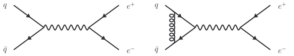
The coefficients of this expansion are the building blocks for the calculation of higher- order corrections to the cross section [143, 144]. The individual terms contributing to the calculation of M^(l)_{f i} have a diagrammatic representation in terms of so-called Feynman diagrams. These are graphs comprised of a specific set of edges and vertices connecting the initial and final state external legs, which is illustrated in Fig. 2.1 by the Drell–Yan process q¯q → e⁺e⁻. The allowed vertices and edges are determined

e⁻ e⁺ q

¯

q e⁻

e⁺ q

¯ q

Figure 2.1: Drell–Yan tree level and one-loop Feynman diagrams.

by the specific quantum field theory via a set of rules known as Feynman rules, which translate Feynman diagrams into their corresponding analytic expressions.

Generally, each additional loop in a Feynman diagram raises the power of the coupling strength in the corresponding analytic expression by one. As a consequence, only Feynman diagrams of a fixed loop order contribute to a given order in the perturbative expansion of a matrix element. In practice, Feynman diagrams provide a convenient way to generate the analytic representation of a given matrix elementM^(l)_{f i}. First, all Feynman diagrams with the given loop order and the right initial and final state are generated. These diagrams are then converted into analytic expressions by virtue of

6

(17)

2.1 From cross sections to Feynman integrals

the Feynman rules.

2.1.2 Dimensionally regulated Feynman integrals

The independent loops in a Feynman diagram are each associated with the integration over an unconstrained so-calledloop momentum. In general, theseFeynman integrals are of the form

 ^L



k=1

d^dlk

iπ^d/2

l^µ₁¹· · ·l^µ₁^r¹ · · ·l^κ_L¹· · ·l^κ_L^rL

P₁· · ·P_t , (2.5) where the inverse propagators P_i are given by¹

P_i =q_i²−m²_i, (2.6)

with m_i denoting the mass of the propagator and q_i being a linear combination of the loop momenta and the momenta of the initial and final state particles, which are referred to asexternal momenta. Since momentum conservation always allows to eliminate one of the external momenta, the term external momenta is in the following understood to refer to the remainingN_ex momenta after momentum conservation has been enforced. A typical example of a one-loop Feynman integral is given by

I^µ(p²) =

 d^dl iπ^d/2

l^µ

[l²−m²][(l−p)²−m²], (2.7) which corresponds to the Feynman diagram in Fig. 2.2. The naive evaluation of

p p

Figure 2.2: One-loop massive bubble integral.

Feynman integrals in four space-time dimensions leads, in general, to divergent results. Therefore, it is necessary to regularize these integrals. While there are several different regularization schemes available, modern calculations almost exclusively em- ploy variants of dimensional regularization [145]. In dimensional regularization, the four-dimensional loop integrations are rendered convergent by promoting them to integrations in

d= 4−2ϵ (2.8)

1An additional term of+iδ in the inverse propagator ensuring the correct time-ordering of the propagator by shifting its poles away from the real axis is omitted here and in the following.

(18)

dimensions. The divergencies in four dimensions are then reflected by poles in the regulator ϵ. The integration over non-integer dimensional vector spaces is, of course, not to be understood literally. Instead, d-dimensional integration can be defined as a functional of the integrand satisfying the following axioms [146]:

Linearity:



d^dl[af(l) +bg(l)] = a



d^dlf(l) +b



d^dlg(l), a, b∈C, (2.9) Scaling:



d^dlf(sl) = |s^−d|



d^dlf(l), s∈C, (2.10) Translation invariance:



d^dlf(l+q) =



d^dlf(l), q= const., (2.11) which resemble properties of ordinary integration if d is a positive integer. The axioms above can be shown [146, 147] to uniquely fix the values of all dimensionally regulated integrals up to a universal normalization, and therefore all explicit constructions of such a functional must yield equivalent results up to normalization.

The universal normalization is often fixed by defining the value of the integral over the (d−1)-dimensional unit sphere



dΩd−1 := 2π^d/2 Γ_d

2

, (2.12)

which also holds for ordinary integration in positive integer dimensions. In practice, it is rarely necessary to resort to an explicit construction of the integration functional². Instead, it is often sufficient to use the axioms above and some additional properties derived from them. In particular, the integration-by-parts [88, 89] property given by Integration-by-parts:



d^dl ∂

∂l^µf(l) = 0, (2.13)

is widely used in practice, as will be explained in Sec. 2.2. The properties outlined above are sufficient for the purposes of this thesis; for a more extensive account of the properties of Feynman integrals the reader is referred to [147, 148].

2Explicit constructions may be obtained by a parametric representation of Feynman integrals [148]

or by a prescription using integrations over finite dimensional subspaces of an infinite dimensional vector space [147].

8

(19)

2.1 From cross sections to Feynman integrals

2.1.3 The projection method

In the calculation of matrix elements, the tensor structures in the numerator of the Feynman integrals in Eq. (2.5) are either contracted with loop momenta, external momenta, polarization vectors or with Dirac gamma matrices. This section presents a technique frequently employed in multi-loop calculations to separate the spin degrees of freedom from the loop integrals. As a result, all loop momenta in the numerator of the Feynman integrals are only contracted with either loop momenta or external momenta. These scalar products in the numerators can then be reduced to a minimal set ofirreducible scalar products.

The first step is to identify an independent set of spin structures D_j sufficient to decompose the matrix element (cf. e.g., [149, 150])

M^(l)_{f i} =

j

m_jD_j. (2.14)

An efficient way to organize the computation of the scalar coefficientsm_j is to define projection operators Pj to project the Feynman diagrammatic representation of the matrix element onto the spin structures. The projectors can be decomposed with respect to the basis of spin structures:

P_j =

k

c_jkD^†_k. (2.15)

The coefficients c_jk are determined by the condition



spins

P_jM^(l)_{f i} =

k,r

c_jk 

spins

D_k^†D_rm_r=m_j. (2.16) It is convenient to define the matrix

D_ij = 

spins

D^†_iD_j, (2.17)

which allows to express the coefficients of the projectors through its inverse c_ij =

D⁻¹

ij. (2.18)

Using the representation of M^(l)_{f i} in terms of Feynman diagrams, the contribution of each Feynman diagram to the coefficients m_j can be extracted by applying the respective projectors as in Eq. (2.16). The resulting scalar coefficients m_j are linear

(20)

combinations of Feynman integrals of the form

 ^L



k=1

d^dl_k iπ^d/2

Q^−ν_t+1^t+1· · ·Q^−ν_t+N^t+Ns

s

P₁· · ·P_t , (2.19) with non-positive integer powers ν_t+1, . . . , ν_t+N_s. The numerator factors Q_i are given by the

Ns = L(L+ 1)

2 +NexL (2.20)

different scalar products of loop momenta and external momenta, involving at least one loop momentum. The inverse propagators P₁, . . . , P_t are independent linear combinations of the scalar products Q_i and terms independent of the loop momenta.

Therefore, there are N_s−t linear combinations of the scalar productsQ_i and terms independent of the loop momenta which are linearly independent of the inverse propagators. Upon choosing such a set of N_s −t so-called irreducible scalar products P_t+1, . . . , P_N_s, the integrals in Eq. (2.19) can be uniquely written as linear combinations of the integrals

I(ν₁, . . . , ν_N_s) =

 ^L



k=1

d^dl_k iπ^d/2

P_t+1^−ν^t+1· · ·P_N^−ν^Ns

s

P₁^ν¹· · ·P_t^ν^t , (2.21) where the powers ν_i of the inverse propagators are now allowed to assume any integer value³. In state-of-the-art computations, the number of integrals of the form in Eq. (2.21) necessary to express the whole matrix element is often of the order of several thousands or more. Thus, it is clearly desirable to treat these with an automatized procedure rather than attempting a case by case analysis.

2.2 Reduction to master integrals

The integrals of the form in Eq. (2.21) are related by a class of linear relations known as integration-by-parts (IBP) identities, which allow to express all such integrals as linear combinations of a relatively small number of so-called master integrals. As a result of this reduction, it is sufficient to evaluate only the master integrals. This section reviews the basic concepts related to the IBP reduction as well as some aspects of the practical organization of such calculations.

3For one-loop integrals, there are no irreducible scalar products sinceNs=t. This fact is exploited in the Passarino–Veltman [151] reduction procedure, which is widely used in one-loop calculations to relate tensor integrals to scalar integrals.

10

(21)

2.2 Reduction to master integrals

2.2.1 Topologies and sectors

It is beneficial to group the integrals occurring in a particular multi-loop calculation into sets of integrals that can be expressed by the same set of propagators and irreducible scalar products. Allowing for arbitrary integer powers of the inverse propagators and non-positive integer powers of the irreducible scalar products, each of these sets contains an infinite number of integrals of the form in Eq. (2.21). These infinite sets of integrals are calledtopologies⁴. The integrals within a given topology can be further divided into differentsectors, where a sector is a set of integrals which share the same set of propagators with positive exponent. Therefore, there are 2^t sectors in a topology witht propagators. A sector is said to be asubsector of another sector if its set of propagators is a subset of the other sector’s set of propagators.

Since two sectors may have disjoint sets of propagators, the sector-subsector relation defines only a partial ordering on the set of sectors. This partial ordering can be turned into a total ordering by defining an integer-valued function on the integrals of the topology:

ID[I] =

t



k=1

2^k−1Θ(ν_k), (2.22)

Θ(x) =

1 x >0,

0 x≤0. (2.23)

This function is constant on sectors, and therefore it can be understood as assigning an integer to each sector, calledsector-id. Moreover, the sector-id is compatible with the partial ordering induced by the sector-subsector relation, because the sector-id of a sector is always greater than the sector-ids of all of its subsectors. Note that the definition of the sector-id depends on the ordering of the propagators.

2.2.2 Integration by parts identities

While a topology contains an infinite number of integrals, there also exists an infinite number of linear relations among them. These integration-by-parts (IBP) relations arise from the property in Eq. (2.13) of dimensionally regularized Feynman integrals [88, 89], which can be cast in the form

 ^L



k=1

d^dl_k iπ^d/2

∂

∂l_j^µ



q^µP_t+1^−ν^t+1· · ·P_N^−ν_s^Ns P₁^ν¹· · ·P_t^ν^t



= 0, j = 1, . . . , L. (2.24) This relation holds for any value of the propagator powers and forqbeing any loop or external momentum. The derivative in the integrand can be carried out explicitly to

4Some authors also use the termintegral family.

(22)

generate a relation between integrals with different powers of the inverse propagators and irreducible scalar products. Using the fact that all scalar products which may occur due to the contraction with q can be written as a linear combination of the inverse propagators and irreducible scalar products, Eq. (2.24) can be expressed as a linear combination of integrals of the same topology with their propagator powers possibly lowered or raised by one:



j

c_jI_j(ν₁+ ∆^j₁, . . . , ν_N_s + ∆^j_N

s) = 0, ∆^j_i ∈ {−1,0,1}. (2.25) The coefficients of these relations are linear functions of the scalar products of external momenta, the internal masses and the space-time dimension d. Since there is one IBP relation for each allowed value of the powers ν_i and each choice of q and the derivative, there exists an infinite number of such relations between the infinite number of integrals in each topology.

It has been shown that by virtue of the IBP relations all integrals in a topology can be expressed as a linear combination of a finite number [152, 153] of integrals with the coefficients being rational functions of the external momenta, the masses and d.

The choice of this finite basis of so-called master integrals is not unique. In fact, the master integrals can be chosen to be any set of linear combinations of integrals of the form in Eq. (2.21) that is both independent with respect to the IBP relations and suffices to express all other integrals.

The following one-loop integral illustrates the use of IBP relations and will be used in later sections of this chapter as well. The integral topology is defined by its two propagators

I(ν₁, ν₂) =

 d^dl iπ^d/2

1

[l²−m²]^ν¹[(l−p)²−m²]^ν², (2.26) which corresponds to the Feynman diagram in Fig. 2.2. There is no need for additional irreducible scalar products in this situation because, for L = 1 and N_ex = 1, the numberN_s = 2of possible scalar products is equal to the number of propagators.

Both scalar products involving the loop momentuml can thus be expressed as linear combinations of the inverse propagators:

l² =P₁ +m², (2.27)

l·p= 1

2(P₁−P₂+p²). (2.28)

12

(23)

In order to generate IBP relations, consider Eq. (2.24) for q=l 0 =

 d^dl iπ^d/2

∂

∂l^µ

 l^µ 1

P₁^ν¹P₂^ν²



(2.29)

=d·I(ν₁, ν₂) +

 d^dl iπ^d/2l^µ ∂

∂l^µ 1

P₁^ν¹P₂^ν² (2.30)

=d·I(ν₁, ν₂)−ν₁

 d^dl iπ^d/2

2l²

P₁^ν¹⁺¹P₂^ν² −ν₂

 d^dl iπ^d/2

2(l²−l·p)

P₁^ν¹P₂^ν²⁺¹ . (2.31) The scalar products in the numerators can be rewritten in terms of the propagators by virtue of Eqs. (2.27) and (2.28)

0 = (d−2ν₁−ν₂)I(ν₁, ν₂)−2ν₁m²I(ν₁+ 1, µ₂) (2.32)

−ν₂I(ν₁−1, ν₂+ 1)−ν₂(2m²−p²)I(ν₁, ν₂+ 1).

In addition to these IBP relations, the integral topology also enjoys the symmetry I(ν₁, ν₂) =I(ν₂, ν₁), (2.33) which corresponds to the change

l→ −l−p (2.34)

of the loop momentum integration variable in Eq. (2.26). This symmetry and the IBP relations are sufficient to relate all integrals of the topology to two master integrals, which may be chosen to be

g₁ =I(1,0), g₂ =I(1,1). (2.35) For instance, by setting ν₁ = 1 and ν₂ = 0 in Eq. (2.32), the integral I(2,0) can be reduced to the master integralI(1,0):

I(2,0) = (d−2)

2m² I(1,0). (2.36)

Using this relation and the IBP relation obtained from Eq. (2.32) for ν₁ = ν₂ = 1, the integral I(2,1) is reduced to the master integrals as follows:

I(2,1) = (d−3)

(4m²−p²)I(1,1)− (d−2)

2m²(4m²−p²)I(1,0). (2.37) The reduction relations Eq. (2.36) and Eq. (2.37) are sufficient to calculate the differential equation of this topology, which is demonstrated in Sec. 2.3. In practice,

(24)

the IBP reduction is used to generate such relations for all integrals occurring in the matrix element of interest.

2.2.3 Lorentz invariance identities

The Lorentz invariance of the integrals in Eq. (2.21) implies a further set of relations [92], which is widely used in practice for the reduction to master integrals. In addition to that, these relations are useful for the differentiation of Feynman integrals with respect to kinematic invariants and are therefore reviewed in the following.

Consider the action of an infinitesimal Lorentz transformation

Λ^µ_ν =δ^µ_ν +ω^µ_ν, ω^µ_ν =−ω^ν_µ (2.38) on one of the N_ex external momenta

p^µ′_j = Λ^µ_νp^ν_j =p^µ_j +ω^µ_νp^ν_j. (2.39) Then, Lorentz invariance implies for any scalar integral I that

I(p_j) =I(p^′_j) (2.40)

=I(p_j) +ω^µ_ν

Nex



j=1

p^ν_j ∂

∂p^µ_jI(p_j) (2.41)

holds for all infinitesimal ω^µ_ν. Using the antisymmetry of ω^µ_ν, the above equation implies

Nex



j=1

 p_jν ∂

∂p^µ_j −p_jµ ∂

∂p^ν_j



I(p_j) = 0, (2.42)

which can be turned into scalar relations by contracting with antisymmetric combinations of external momenta. For instance, for Nex = 2, there is only the identity

(p^ν₁p^µ₂ −p^µ₁p^ν₂)

2



j=1

 p_jν ∂

∂p^µ_j −p_jµ ∂

∂p^ν_j



I(p_j) = 0. (2.43) Since at mostdof theN_exexternal momenta can be linearly independent, the number of linearly independent external momenta after using momentum conservation is given by N_ind =min(d, N_ex). Thus, there are N_ind(N_ind−1)/2 independent Lorentz invariance relations of the above form, because this is the number of antisymmetric combinations of the independent external momenta.

It has been shown [154] that the Lorentz invariance identities are not linearly independent of the IBP relations and thus not strictly necessary for the reduction to master integrals. In practice, however, they can speed up the reduction process and

14

(25)

are therefore widely used.

2.2.4 Systematic reduction strategies

As mentioned before, the number of Feynman integrals contributing to a particular matrix element can be relatively large. It is thus desirable to automate their reduction to master integrals. One strategy to attempt an automatized reduction is to combine IBP identities with symbolic propagator powers, such as Eq. (2.32), into symbolic reduction rules [130, 131, 154–156], which may be interpreted as ladder operators acting on the propagator powers. Applied recursively, the reduction rules relate all integrals of a given topology to master integrals. Once the reduction rules have been found, the reduction itself is very efficient. However, a systematic way of constructing symbolic reduction rules has not yet been found, and thus implementations of this strategy have to resort to heuristic methods.

Laporta proposed [157] the completely systematic but rather brute-force strategy of considering the IBP relations for a finite range of integer values of the propagator powers. The integrals within this range are called seed integrals. For each seed integral, Eq. (2.24) generates an IBP relation for all of the L(N_ex +L) choices of q and the derivative, which usually results in a large system of equations for the seed integrals. The next step is to essentially perform a Gaussian elimination to triangularize the system of equations. By defining a so-called Laporta ordering on the integrals that reflects their complexity, the elimination can be performed such that more complex integrals are eliminated in favor of less complicated ones. Usually, this ordering is chosen to be compatible with the ordering of the sectors induced by the sector-id. If this is the case, every integral is reduced to master integrals from the same or lower sectors.

Variations of the Laporta strategy have been implemented in numerous publicly available programs [127–129, 131, 132, 135]. In practice, these calculations suffer from the fact that most of the IBP relations generated from the seed integrals are linearly dependent. In fact, in the limit of large ranges of seed integrals only one relation perL(N_ex+L)IBP relations can be linearly independent, since the number of master integrals remains fixed. The unnecessary computations due to linearly dependent IBP relations can be avoided by eliminating such relations with finite field techniques [135, 158, 159] prior to the Gaussian elimination step. By mapping the time-consuming computations over the field of rational functions to the modular arithmetic of finite fields, the linearly dependent relations can be eliminated very efficiently.

Altogether the IBP reduction to master integrals can be considered as a concep- tionally solved problem, but in practice, the computations are often limited by the computational resources at disposal.

(26)

2.3 Differential equations of Feynman integrals

After the reduction to master integrals, it remains to evaluate the relatively small number of master integrals as functions of the kinematic invariants. This problem has been approached in numerous ways, but despite many advances, a general solution has not yet been found and still appears to be far out of reach. However, in recent years the method of differential equations [90–92] has been successfully applied to a large class of Feynman integrals. This development has been enabled by the observation [65] that a particular choice of the basis of master integrals drastically simplifies the solution of the corresponding differential equation. The key ideas of the differential equations approach are reviewed in this section.

2.3.1 Differentiation of Feynman integrals

The master integrals are functions ofN_ex external momenta and a number of internal mass scales. Lorentz invariance implies that Feynman integrals can only depend on the external momenta via kinematic invariants X₁, . . . , X_E, which are independent Lorentz invariant functions of the external momenta. In addition to these invariants, the integrals may also depend on internal masses X_E+1, . . . , X_Q. The goal is to evaluate the master integrals as functions of all kinematic invariants X₁, . . . , X_Q.

The basic idea of the method of differential equations is to derive a system of differential equations for the master integrals by calculating the derivatives of all master integrals with respect to the kinematic invariants X₁, . . . , X_Q and then solve it in terms of known functions. The derivative of an integral with respect to one of the internal massesX_E+1, . . . , X_Qis straightforward to perform in the representation Eq. (2.21) since the mass dependence is explicit. By interchanging the derivative with the loop momentum integration [160] and using the product rule on the propagators, the derivative results in a linear combination of integrals from the same sector with possibly raised propagator powers.

The derivatives with respect to the kinematic invariantsX₁, . . . , X_E are related to the derivatives with respect to the external momenta by the chain rule

∂

∂p^µ_i =

E



j=1

∂X_j

∂p^µ_i

∂

∂X_j, i= 1, . . . , N_ex. (2.44) Each of these relations can be contracted with any of the N_ind independent external momenta to give the scalar relations

p^µ_k ∂

∂p^µ_i =

E



j=1

p^µ_k∂Xj

∂p^µ_i

∂

∂X_j, i= 1, . . . , N_ex, k= 1, . . . , N_ind. (2.45) The contracted derivatives on the left-hand side are related by Lorentz invariance

16

(27)

2.3 Differential equations of Feynman integrals

relations of the form in Eq. (2.43), if they are applied to Lorentz invariant scalars.

Therefore, only

NexNind− N_ind(N_ind−1)

2 (2.46)

of the relations in Eq. (2.45) are independent, which precisely corresponds to the numberEof independent Lorentz invariants that can be formed from theN_exexternal momenta.

Thus, after choosing a set of E independent relations from Eq. (2.45), these can be solved for theE derivatives with respect to the kinematic invariants X₁, . . . , X_E, which are then expressed as linear combinations of the contracted derivatives with respect to the external momenta. This allows to evaluate the derivatives with respect to the kinematic invariants by acting on the integrals with the derivatives with respect to the external momenta, which can be interchanged with the integration and evaluated directly on the integrand.

The derivative of the integrand with respect to the external momenta and the subsequent contraction with an external momentum can be written as a linear combination of inverse propagators and irreducible scalar products, which results in a linear combination of integrals with shifted propagator powers. Note that this oper- ation can never generate new propagators with positive powers. Thus, the derivative of a scalar integral with respect to an external invariant can always be written as a linear combination of integrals from the same or lower sectors.

As an example, consider the derivative ofg₂ =I(1,1)with respect to the kinematic invariants=p². There is only one relation of the form in Eq. (2.45)

p^µ ∂

∂p^µ =p^µ ∂s

∂p^µ

∂

∂s = 2s ∂

∂s. (2.47)

The derivative with respect to p^µ raises the power of P2 and generates a linear combination of scalar products in the numerator upon contraction withp^µ. By virtue of Eq. (2.28), the scalar productl·pis rewritten in terms of the inverse propagators, which allows to express the derivative as a linear combination of scalar integrals with shifted propagator powers

p^µ∂I(1,1)

∂p^µ =

 d^dl iπ^d/2

2l·p−2p²

P1P₂² =I(0,2)−I(1,1)−p²I(1,2). (2.48) Solving Eq. (2.47) for the derivative with respect tos leads to

∂I(1,1)

∂s = 1

2s

I(0,2)−I(1,1)

−I(1,2). (2.49)

Since the master integral g₁ =I(1,0) does not depend on the external momentum,

(28)

its derivative with respect to s vanishes due to Eq. (2.47)

∂I(1,0)

∂s = 0. (2.50)

The strategy described here to calculate derivatives of Feynman integrals with respect to their invariants in terms of integrals of the same topology is completely algorithmic and has for example been implemented in [128, 129].

2.3.2 Differential equations and canonical bases

In the previous section, it has been shown that derivatives of Feynman integrals with respect to the kinematic invariants can be expressed as linear combinations of scalar integrals from the same or lower sectors. By applying the IBP reduction to those integrals, derivatives of scalar integrals can always be written as linear combinations of master integrals. If the differentiated integrals are master integrals, this results in a coupled first-order linear system of differential equations for the master integrals. Solving these differential equations in terms of known functions, and imposing appropriate boundary conditions then achieves the goal of evaluating the master integrals as functions of the kinematic invariants.

In the case of the previously considered example, the scalar integrals on the right- hand side of Eq. (2.49) are reduced to master integrals with Eq. (2.36) and Eq. (2.37)

∂g₂

∂s = (d−2)

s(4m²−s)g₁− 1 2

1

s + (d−3) (4m²−s)



g₂, (2.51)

∂g₁

∂s = 0. (2.52)

A differential equation of this form can be derived for all of the kinematic invariants.

However, the dependence of the master integrals on one of the kinematic invariants can always be reconstructed from the mass dimension dim(I) of the integral, which is easily determined by counting the powers of its propagators and irreducible scalar products. Then, by choosing any of the kinematic invariants, for instance, X_Q, the basis of master integrals can be normalized such that all integrals have mass dimension zero

f_i = (X_Q)^−dim(gⁱ^)/dim(X^Q⁾g_i. (2.53) Due to their trivial mass dimension, the integralsf_i must be functions of M =Q−1 dimensionless functions of the kinematic invariants. These can, for example, be chosen to be the dimensionless ratios

x_i = X_i

X_Q^dim(Xⁱ^)/dim(X^Q⁾

, i= 1, . . . , M. (2.54)

18

(29)

Using dimensionless master integrals is straightforward in practice and reduces the number of variables by one.

The integrals in the above example depend on the two dimensionful invariants s and m. By choosing m as the variable to be factored out, a dimensionless basis of master integrals is obtained by

f1 = (m)^−(d−2)e^ϵγÊϵg1, f2 = (m)^−(d−4)e^ϵγÊϵg2, (2.55) where ϵ denotes the dimensional regulator as introduced in Eq. (2.8). The integral vector has been multiplied with the overall factore^ϵγÊ because it conveniently removes terms involving the Euler–Mascheroni constant γE from the expansion of f. The⃗ additional factor of ϵ ensures that the ϵ-expansion of the f_i starts at a non-negative order. Due to their trivial mass dimension, the integrals f⃗ must be functions of the dimensionless ratio

x= s

m². (2.56)

Using the chain rule and Eq. (2.49) yields for the derivatives with respect to x

∂f₂

∂x =m^6−d∂g₂

∂s =m^6−d

 (d−2)

s(4m²−s)g₁− 1 2

1

s + (d−3) (4m²−s)

 g₂



(2.57)

= (d−2)

x(4−x)f₁−1 2

1

x + (d−3) (4−x)



f₂ (2.58)

and ∂f₁

∂x =m^4−d∂g₁

∂s = 0. (2.59)

Upon replacing the dimension with d = 4−2ϵ and considering the full vector of master integrals, the derivative can be written as

∂ ⃗f

∂x =

 0 0

(2−2ϵ)

x(4−x) −¹₂

1

x + ^(1−2ϵ)_(4−x)



f .⃗ (2.60)

For a general topology withmmaster integrals depending onM dimensionless invariants, the derivative can be taken with respect to all dimensionless invariants, which results in a coupled system of linear differential equations for the master integrals

∂_if(ϵ,⃗ {x_j}) =a_i(ϵ,{x_j})f⃗(ϵ,{x_j}), i= 1, . . . , M, (2.61) with the a_i(ϵ,{x_j}) being m × m matrices of rational functions in the kinematic invariants {x_j} and ϵ. The fact that the matrices a_i(ϵ,{x_j}) are rational functions of the kinematic invariants and ϵ is evident from the structure of the integration- by-parts relations in Eq. (2.24). In Sec. 2.3.1 it was argued that the derivative of a Feynman integral can be represented as a linear combination of integrals from

(30)

the same or lower sectors. If the Laporta ordering is compatible with the sector structure, each of these integrals has a representation in terms of master integrals from the same or lower sectors. Altogether this leads to a lower-left block-triangular form of thea_i(ϵ,{x_j})matrices if the vector of master integralsf⃗is ordered according to the sector-id. It is convenient to use the more compact differential notation for the system of differential equations in Eq. (2.61)⁵

df⃗(ϵ,{x_j}) =a(ϵ,{x_j})f(ϵ,⃗ {x_j}), (2.62) with

a(ϵ,{xj}) =

M



i=1

ai(ϵ,{xj})dxi. (2.63) The choice of the basis of master integrals is not unique. Changing the basis of master integrals to a new basisf⃗^′ that is related to the original basis by an invertible transformation T

f⃗=T(ϵ,{x_j})f⃗^′, (2.64) as suggested in [65], leads to a transformation law for a(ϵ,{x_j}):

a^′ =T⁻¹aT −T⁻¹dT. (2.65)

In the following, some notation and terminology related to particular forms ofa(ϵ,{x_j}) is introduced. The differential equation is said to be in dlog-form if the differential form a(ϵ,{xj}) can be written as

a(ϵ,{x_j}) = dA(ϵ,{x_j}), (2.66) with

A(ϵ,{x_j}) =

N



l=1

A_l(ϵ) log(L_l({x_j})). (2.67) Here L_l({x_j}) denotes functions of the invariants, and the A_l are m×m matrices, which solely depend on ϵ. The set of functions

A={L1({xj}), . . . , LN({xj})} (2.68) is commonly referred to as the alphabet of the differential equation. The individual L_l({x_j}) are called letters of the differential equation. In [65] it was observed that with a suitable change of the basis of master integrals it is often possible to arrive at

5The differential equation Eq. (2.62) is completely determined by the differential forma(ϵ,{xj}).

Therefore,a(ϵ,{xj})is also frequently referred to as the differential equationin the following.

20

(31)

a dlog-form in which the dependence onϵ factorizes a(ϵ,{xj}) =ϵdA({x˜ j}) =ϵ

N



l=1

A˜ldlog(Ll({xj})), (2.69)

withA˜_l being constant m×m matrices. In this form, which is called canonical form or ϵ-form, the integration of the differential equation simplifies significantly as will be shown in Sec. 2.4. A basis of master integrals for which the differential equation assumes a canonical form is called acanonical basis.

Note that in the derivation of the differential equation Eq. (2.62) described in the previous sections, the master integrals and the invariants {x_j} can always be chosen such that the resulting differential form a(ϵ,{x_j}) is rational in the invariants and the regulator. For rational transformations to the canonical form, it follows that the resulting canonical form is rational as well and thus the letters are polynomials in the invariants. However, there are differential equations for which the transformation to a canonical form necessarily contains roots of polynomials in the invariants, which may lead to letters containing these roots.

The differential equation Eq. (2.60) of the example considered above can also be transformed into canonical form. To this end, it is advantageous to first change the coordinates to

x=−(1−y)²

y , (2.70)

because this allows for a rational transformation of the differential equation to a canonical form to exist. With respect to the new coordinatey, the differential equation Eq. (2.60) reads in differential form

df⃗=

 0 0

1−ϵ

−1+y +^−1+ϵ_1+y _−1+y⁻¹ +_y^ϵ +^1−2ϵ_1+y



dy ⃗f . (2.71) The transformation given by

T =

 1

1−ϵ 0

1 1−2ϵ

1+y 2(1−2ϵ)(−1+y)

