IHS Economics Series Working Paper 330
September 2017
Linear Time Iteration
Pontus Rendahl
Impressum Author(s):
Pontus Rendahl Title:
Linear Time Iteration ISSN: 1605-7996
2017 Institut für Höhere Studien - Institute for Advanced Studies (IHS) Josefstädter Straße 39, A-1080 Wien
E-Mail: o ce@ihs.ac.atffi Web: ww w .ihs.ac. a t
All IHS Working Papers are available online: http://irihs. ihs. ac.at/view/ihs_series/
This paper is available for download without charge at:
https://irihs.ihs.ac.at/id/eprint/4351/
Linear Time Iteration
Pontus Rendahl
†University of Cambridge, CfM, and CEPR May 16, 2017
Abstract
This paper proposes a simple iterative method – time iteration – to solve linear rational expec- tation models. I prove that this method converges to the solution with the smallest eigenvalues in absolute value, and provide the conditions under which this solution is unique. In particular, if conditions similar to those of Blanchard and Kahn (1980) are met, the procedure converges to the unique stable solution. Apart from its transparency and simplicity of implementation, the method provides a straightforward approach to solving models with less standard features, such as regime switching models. For large-scale problems the method is 10-20 times faster than existing solution methods.
†The author would like to thank SeHyoun Ahn, Ben Moll, Wouter J. den Haan, Greg Kaplan, Tamas Papp, and Michael Reiter for helpful comments and suggestions. The usual disclaimer applies. E-mail:
pontus.rendahl@gmail.com.
1 Introduction
Solving linear(ized) rational expectation models is a cornerstone in any macroeconomist’s toolkit.
In a seminal paper, Blanchard and Kahn (1980) provided the foundations for how to solve a certain class of such models, and how to verify the stability and uniqueness of a solution. As their class of models, however, was confined to deal with frameworks absent of intratemporal relationships – such as accounting identities, or optimal static choices – a plethora of alternative solution methods has emerged to (successfully) address this seemingly trivial problem.
1Nevertheless, while these alternative methods are both fast and accurate, they are quite esoteric and lack in transparency.
2As a consequence, it is common for most researchers to instead rely on pre-canned routines.
This paper takes a step forward by providing a method that improves both the simplicity and transparency of solving linear rational expectation models, without any loss of applicability or efficiency. In particular, I propose an iterative schedule for which the sequence of approximate solutions converges to the solution to the problem with the smallest eigenvalues in absolute value, and provided conditions under which the solution is unique and stable.
The logic underlying the procedure is simple enough to be described in words. Envisage an agent having a certain amount of an asset, facing the choice between how much of this asset to consume and how much to save. An optimal choice would trade off the marginal benefit of saving (future consumption) with its marginal cost (forgone current consumption). The resulting optimal decision is implied by a linear(ized) second-order difference equation.
However, while the marginal cost associated with any choice is clear – since both the current value of the asset is known, and the choice of saving pins down current consumption – the marginal benefit is not readily known. In particular, the future marginal benefit of saving depends on the optimal saving choice in the future. Thus, an optimal choice today can only be determined under the condition that the optimal choice in the future is known; thus the problem amounts to finding a fixed point. To solve this problem, this paper proposes to guess for the optimal choice of saving in the future as a linear function of the associated state (which is given by the optimal choice in the present). Given such a guess, the optimal choice in the present is then trivially given by solving a linear equation. However, the current optimal choice provides us with another suggestion regarding future optimal behavior, and the guess is updated accordingly.
This procedure is shown to be convergent, and, as previously mentioned converges to the solution with the smallest eigenvalues in absolute value. After having proved the papers main
1Examples include Klein (2000), Uhlig (2001), Christiano (2002), and Sims (2002). King and Watson (2002) show thatanylinearized system can be recast into the original formulation of Blanchard and Kahn (1980).
2For instance, Sims (2002) writes “While these more general solution methods are themselves harder to understand, they shift the burden of analysis from the individual economist/model-solver toward the computer, and are therefore useful.”
Propositions, I subsequently illustrate how the method works using four examples, including problems in continuous-time, and regime switching models. Lastly, I compare the performance of the algorithm to existing solution methods, and find that the proposed method is 10-20 times faster for large-scale problems. Thus, the method may provide useful in addressing problems such as those considered in Reiter (2009).
2 Method
The model of interest is given by
Ax
t−1+ Bx
t+CE
tx
t+1+ u
t= 0, (1) where x
tis an n
×1 vector containing endogenous and exogenous variables, u
tis an n
×1 vector of mean-zero disturbances, and A, B and C are conformable matrices.
We are interested in a recursive solution of the type x
t= Fx
t−1+ Qu
t. Inserting this rule into equation (1) gives,
Ax
t−1+ Bx
t+ CFx
t+ u
t= 0.
Thus, the matrix Q is given by
Q =
−(B+ CF )
−1, (2)
and F must be the solution to the quadratic matrix equation (cf. Uhlig (2001))
A + BF + CF
2= 0. (3)
If F is known, finding Q is a trivial operation following equation (2). From hereon, the focus of this paper is therefore on solving equation (3).
A solution to equation (3) is called a solvent.
Definition 1.
A solvent S
1of (3) is a dominant solvent if
λ(S
1) =
{λ1, . . . ,
λn}and
|λn|>
|λn+1|where the eigenvalues are ordered according to
|λ1| ≥ |λ2| ≥
. . .
≥ |λ2n|.A solvent S
2of (3) is a minimal solvent if
λ(S
2) =
{λn+1, . . . ,λ
2n}and
|λn|>
|λn+1|.Theorem 1.
(Higham and Kim (2000), Theorem 6) Suppose that the Eigenvalues that solves
(A + Bλ + Cλ
2)x = 0, (4)
satisfy the ordering and conditions of Definition 1, and that corresponding to
{λi}ni=1and
{λi}2ni=n+1there are two sets of linearly independent eigenvectors
{v1, . . . , v
n}and
{vn+1, . . . ,v
2n}, then thereexist a dominant, S
1, and a minimal solvent, S
2, of (3).
Theorem 2.
(Gohberg, Lancaster and Rodman (1982), Theorem 4.1) If a dominant and a minimal solvent exist they are unique.
2.1 Time iteration
The main equation of interest is given by
3Ax
t−1+ Bx
t+ Cx
t+1= 0.
Suppose we have a candidate solvent, F
n. Then consider solving the following problem for x
tAx
t−1+ Bx
t+CF
nx
t= 0.
The solution is trivially given by
x
t=
−(B+CF
n)
−1Ax
t−1. Thus, we will therefore update our guess, F
n+1, as
4F
n+1=
−(B+ CF
n)
−1A.
In order to prove that this is a convergent procedure, we will need the following lemma.
Lemma 1.
Let Z
1and Z
2be square matrices such that
min{|λ
|:
λ ∈λ(Z
1)} > max{|λ
|:
λ ∈λ(Z
2)}.
3Recall that it is sufficient to solve the deterministic part of the problem in order to retrieveF. The matrixQthe follows straightforwardly from equation (2).
4Binder and Pesaran (1995), footnote 26, propose a similar iterative procedure, but do not provide any proof of convergence, nor conditions for stability/uniqueness.
Then Z
1is nonsingular and for any matrix norm
i→∞
lim
kZ2ikkZ1−ik= 0 Proof. Gohberg et al. (1982), Lemma 4.9
Proposition 1.
Suppose a dominant, S
1, and a minimal solvent, S
2, exist for equation (3). Then, if the matrix (B + CF
n) is nonsingular for all n, the sequence
{Fn}∞n=0defined as
F
n+1= (B +CF
n)
−1(−A), F
06=S
1, (5) converges to S
2.
Proof. In Appendix A.
The proof of Proposition 1 follows Higham and Kim (2000) quite closely, with some tweaks to fit the purposes of this paper.
The procedure is guaranteed to converge the minimal solvent, S
2. If all the eigenvalues of S
2is less than one in absolute value, S
2is indeed a (stable) solution to the quadratic matrix equation.
Thus a stable solution exist. However, that does not necessarily imply that S
2is the only stable solution. Indeed, the dominant solvent S
1– or some other solvent – may also be stable. To verify that this is not the case, the proposition below provides an iterative procedure to find S
−11. Thus, if the eigenvalues of S
−11are smaller than one in absolute value, the eigenvaluea of S
1is greater than one in absolute value, and S
1is not a stable solution.
Proposition 2.
Suppose a dominant, S
1, and a minimal solvent, S
2, exist. Then, if the matrix (B + A F ˆ
n) is nonsingular for all n, the sequence
{F ˆ
n}, defined byF ˆ
n+1= (B + A F ˆ
n)
−1(−C), (6) converges to S
−11.
Proof. In Appendix A.
Thus, given the (inverse) of a dominant, S
−11, and minimal, S
2, solvent to equation (3) if (i) If max
|λ(S
2)| < 1, and max
|λ(S
−11)| < 1, S
2is the unique stable solution to equation (3).
(ii) If max
|λ(S
2)| > 1 there exist no stable solution.
(iii) If max
|λ(S
−11)| > 1 there are multiple stable solutions.
2.1.1 Singular solvents
One particularly pertinent issue that arises is to which extent the above method can deal with situations in which solvents contain eigenvalues that are zero. It is straightforward to verify that a dominant solvent cannot have those properties, as Definition 1 would not be satisfied. Unfortunately, this is a quite common feature of dynamic systems that contain static relationships, such as accounting identities or the first order conditions of static optimization problems. Fortunately, there is a straightforward workaround to this issue.
Consider the (modified) quadratic matrix equation
AS ˆ
2+ BS ˆ + C ˆ = 0, (7)
with
A ˆ = Cµ
2+ Bµ + A, B ˆ = B +C2µ , C ˆ = C,
where
µrepresents a small positive real number multiplied by a conformable identity matrix. It is straightforward to verify that if S satisfies equation (7), then F = S
−1+
µsatisfies the original quadratic matrix equation (here repeated for exposition)
A + BF + CF
2= 0. (8)
Conversely, any F which satisfies the quadratic matrix equation (8), then S = (F
−µ)
−1satisfies equation (7). It is worth pointing out here that S is indeed nonsingular unless
µhappens to contain an eigenvalue of F. Ruling this scenario out, S is invertible and has no eigenvalues equal to zero.
Proposition 3.
Suppose for some
µequation (7) has dominant, S
1, and a minimal solvent, S
2, such that
|λi(S
1)| > 1/M and
|λi(S
2)| < 1/M. If
µ< M
− |λi(S
−11)|, for i = 1, . . . ,n, then for F = (S
−11+
µ)
(i) F solves the quadratic matrix equation (8).
(ii)
|λi(F )| < M, for i = 1, . . . , n.
(iii) F is the unique solvent satisfying (i) and (ii).
Proof. Part (i). Inserting F = S
−11+
µinto the left-hand side of equation (8) gives A + B(S
−11+
µ) + C(S
−21+ 2S
1µ+
µ2)
= (A + Bµ +Cµ
2) + (B + 2µ )S
−11+CS
1−2= (A + Bµ +Cµ
2)S
21+ (B + 2µ )S
1+C
= 0.
Part (ii). Since
|λi(S
−11)| < M for each i = 1, . . . , n, we have that
|λi
(F )| =
|λi(S
−11) +
µ|≤ |λi
(S
−11)| +
µ<
|λi(S
−11)| + (M
− |λi(S
−11)|)
= M
Part (iii). Suppose there exist an ˆ F
6=F which solves equation (8) such that
|λi( F)| ˆ < M for i = 1, . . . , n. Then ˆ S = ( F ˆ
−µ)
−1solves equation (7). In addition, for any
µ> 0 such that
µ< M
− |λi( F)| ˆ for i = 1, . . . , n we have
|λi
( S ˆ
−1)| =
|λi( F ˆ )
−µ|≤ |λi
( F ˆ )| +
µ<
|λi( F ˆ )| + (M
− |λi( F)|) ˆ
= M.
As a consequence
|λi( S)| ˆ > 1/M for i = 1, . . . , n, which contradicts that S
1is the unique dominant solvent to equation (7). Hence, F is unique.
In practice, Proposition 3 suggests to pick a (small) value
µ; solve equation (7) using Propo- sitions 1 and 2; and then evaluate the interval
M= (max
|λ(S
2)|, min
|λ(S
1)|), to obtain the admissible values of 1/M
∈M. In addition, it ought to be noted that, for practical purposes, there is no harm done in setting
µequal to a very small number, as the convergence properties appear to improve with a lower value of
µ(see the example in Section 3.2.1 below).
Corollary 1.
If (7) has dominant, S
1, and a minimal solvent, S
2, such that
|λi(S
1)| > 1 and
|λi
(S
2)| < 1, with 0 <
µ< 1
− |λi(S
−11)|, for i = 1, . . . ,n. Then, F = S
−11+
µis the unique stable solvent to equation (8).
While Proposition 3 provides useful guidance on how to find and characterize solvents that are
smaller or larger than a certain threshold in absolute value, it is far less useful to find and characterize
solvents that are smaller or larger than a certain threshold on the real line. As stability conditions for continuous time problem regularly require that all eigenvalues are negative, Proposition 4 below provides a solution to this issue.
Proposition 4.
Suppose for some
µ< 0 equation (7) has dominant, S
1, and a minimal solvent, S
2. If
λi(S
1)
≥ −1/µand 0
≤λi(S
2) <
−1/µ, for i = 1, . . . ,n, then for F = (S
−11+
µ)
(i) F solves the quadratic matrix equation (8).
(ii)
λi(F )
≤0, for i = 1, . . . , n.
(iii) F is the unique solvent satisfying (i) and (ii).
Proof. Part (i). See the associated proof for Proposition 3.
Part (ii). Since
λi(S
−11) <
−µfor each i = 1, . . . , n, we have that
λi(F) =
λi(S
−11) +
µ≤ −µ
+
µ= 0.
Part (iii). Suppose there exist an ˆ F
6=F with
λi( F) ˆ
≤0 for all i = 1, . . . , n which solves equation (8). Then S = ( F ˆ
−µ)
−1is a solvent for equation (7), with
λi(S)
∈ {λ:
λ< 0, or
λ ≥ −1/µ},for all i = 1, . . . , n. Suppose that
λi(S) < 0 for some i = 1, . . . , n, then
λ(S),
λ(S
1), and,
λ(S
2) all constitute eigenvalues to the quadratic eigenvalue problem in (4), with the total number of eigenvalues exceeding 2n, which is an impossibility. Thus
λi(S)
≥ −1/µ, for all i = 1, . . . , n.
However, if
λi(S)
≥ −1/µfor all i = 1, . . . , n this contradicts that S
1is unique. Hence, there can not exist an ˆ F
6=F with
λi( F) ˆ
≤0 for all i = 1, . . . , n.
The ideas underlying Proposition 3 and 4 are similar but operate in opposite directions. Proposi- tion 3 requires a perturbation of the system by a sufficiently small amount to ensure that a dominant solvent exists, while at the same time leaving the system sufficiently unperturbed to allow for infer- ence. Conversely, Proposition 4 suggests to perturb the system sufficiently to shift all eigenvalues that were negative in the original system to be the smallest positive roots of the modified system.
3 Examples
This section provides five examples of how to use the proposed method. The first is intended to
show the convergence properties of both S
2and S
−11in the simplest possible case. The second, to
illustrate how to deal with singular solvents using Proposition 3. The third illustrates a model set in
continuous time using Proposition 4. The fourth considers a regime switching model. And the fifth is intended to show the large-scale properties of the method.
Convergence is assumed to be obtained once the absolute maximum error of the quadratic matrix equation is smaller than 1e(−12), which is close to double-precision machine epsilon.
3.1 A second-order difference equation.
Consider the following second-order difference equation 0.75x
t−1−2x
t+ x
t+1= 0.
The associated quadratic equation is
0.75
−2F + F
2= 0,
with dominant, S
1, and minimal solvent, S
2, equal to 1.5 and 0.5, respectively.
Fn
0.5 1 1.5 2
0.2 0.4 0.6 0.8 1 1.2 1.4 1.6 1.8 2
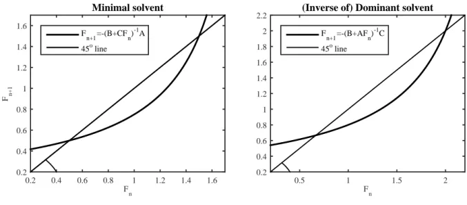
2.2 (Inverse of) Dominant solvent
Fn+1=-(B+AF
n)-1C 45o line
Fn
0.2 0.4 0.6 0.8 1 1.2 1.4 1.6
F n+1
0.2 0.4 0.6 0.8 1 1.2 1.4 1.6
Minimal solvent
Fn+1=-(B+CF
n)-1A 45o line
Figure 1: Mapping ofFntoFn+1.
Figure 1 illustrates the mappings of the iterations F
n+1=
−0.75/(−2+ F
n) (left graph) and F
n+1=
−1/(−2
+ 0.75F
n) (right graph). From the left graph it is clear that for any guess F
0such that F
0< 1.5, the sequence F
nconverges to the minimal solvent 0.5. What is less obvious is that for any F
n> 1.5 the resulting sequence also converges to 0.5.
5The reason is that for any F
n> 2 it follows that F
n+1< 0, which guarantees convergence. Numerically, even at the singularity that arises at F
n= 2 is not a problem either, since most numerical programs interpret 1/0 as infinity and 1/∞
as zero. Thus, even for an initial guess of F
0= 2, the procedure converges to the minimal solvent.
5Notice that lim|F|→∞−0.75/(−2+F) =0.
The only initial guess for which convergence (towards the minimal solvent) does not occur is if F
0= 1.5; that is, if the initial guess for the minimal solvent is equal to the dominant solvent.
The right graph illustrates the convergence properties of the inverse of the dominant solvent.
For any F
0< 2, the sequence F
nconverges to the inverse of the dominant solvent, F = 2/3. In addition, for any F
n> 2.67, F
n+1< 0 and convergence follows. Again, the only initial guess for which convergence (towards the inverse of the dominant solvent) does not occur is if F
0= 2; that is, if the initial guess for the inverse of the dominant solvent is equal to the inverse of the minimal solvent.
3.2 Singular solvents
Consider a variation of the previous problem
0.75y
t−0.5y
t+1= 0,
−2xt
+ x
t−1−y
t= 0, or,
AX
t−1+ BX
t+CX
t+1= 0, with X
t= (y
t, x
t)
0, and
A = 0 0 0 1
!
, B = 0.75 0
−1 −2
!
, C =
−0.5 00 0
!
.
There are three solvents to this problem S
1= 0
−20 1.5
!
, S
2= 0 0
0 0.5
!
, S
3= 1.5 0
−0.75 0.5
!
,
with eigenvalues of (0, 1.5), (0, 0.5), and (0.5, 1.5), respectively. Thus, S
1and S
3represent the unstable solutions, and S
2the (unique) stable solution.
It would be tempting to refer to S
1as the dominant solvent and S
2as the minimal solvent, but
this would be incorrect; both the dominant and minimal solvent have a zero eigenvalue, and do
therefore not satisfy Definition 1. Hence, neither Proposition 1 nor 2 are valid. However, it may still
be interesting to conduct the iterations suggested in Proposition 1 and 2 in order to explore what
they may deliver.
The resulting “inverse” of the “dominant” solvent, S
−11and, “minimal” solvent, S
2are
S
−11= 0.667 0
−0.5
0
!
, S
2= 0 0
0 0.5
!
,
with nonzero eigenvalues of 0.667 and 0.5, respectively. Thus, the nonzero eigenvalue of the inverse of the “dominant” solvent corresponds exactly with the inverse of the nonzero eigenvalue of the unstable solution S
1above; and the nonzero eigenvalue of the “minimal” solvent corresponds exactly with the nonzero eigenvalue of the stable solution – indeed, the procedure correctly identifies the stable solution S
2and also suggests that there exist another solution which is unstable. Furthermore, inspecting S
−11suggests that the unstable solution satisfies
y
t−1= 0.667y
tx
t−1=
−0.5yt. Thus, “inverting” these policy functions gives
y
t=
−2xt−1x
t= 1.5x
t−1, which exactly replicates the unstable solution S
1above.
Is this a coincidence that is particular to this example? My experience tells me that it is not; for a wide range of models and calibrations the procedure delivers a stable solvent, together with a matrix, S
−11, containing the coefficients of the inverse of the unstable policy function.
6However, acknowledging that not every reader may be as convinced by “my experience” as I am, we can invoke Proposition 3 to address this issue.
3.2.1 Using Proposition 3
In order to exploit the results in Proposition 3, we need to pick a value for
µ. Setting µ, conserva-tively, equal to 0.1 gives rise to
A ˆ = 0.07 0
−0.1 0.8
!
, B ˆ = 0.65 0
−1 −2
!
, C ˆ =
−0.5 00 0
!
,
6Provided, of course, that a stable and unstable solution exist. If there is no stable solution – or if both solvents are stable – the procedure still delivers a solvent with the smallest nonzero eigenvalues in absolute value, and a matrix containing the inverse of a solvent with larger eigenvalues in absolute value, provided that the smallest nonzero eigenvalues of the latter strictly exceeds the largest nonzero eigenvalue of the former. Only if these eigenvalues happen to coincide have I run into convergence issues.
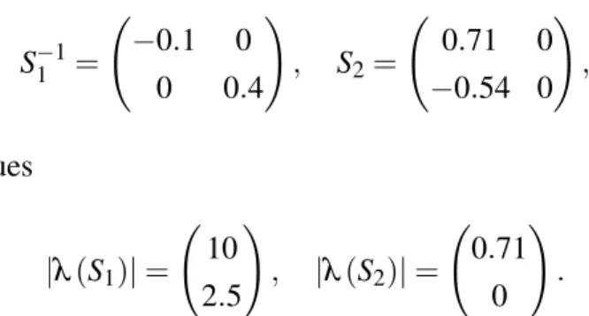
and Proposition 3 delivers the solvents S
−11=
−0.10
0 0.4
!
, S
2= 0.71 0
−0.54 0
!
,
with associated eigenvalues
|λ
(S
1)| = 10 2.5
!
,
|λ(S
2)| = 0.71
0
!
.
Thus S
1is indeed the dominant solvent and S
2is the minimal solvent. Since
µ< 1
−1/2.5, all the conditions of Proposition 3 are met, and F = S
−11+
µis the unique stable solution.
Values of 7
0 0.5 1 1.5
Eigenvalues
0.5 1 1.5 2 2.5 3 3.5
4 6(S
1) 6(S2) 6((S3+7)-1) 6(S1
-1+7) 6(F)
Values of 7
0 0.1 0.2 0.3 0.4 0.5
Iterations
0 10 20 30 40 50
Time (milliseconds)
0 0.4 0.8 1.2 1.6 2 Iterations Time
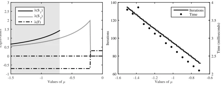
Figure 2: The relationship betweenµ and eigenvalues.
Notes. (Left panel) The black solid line shows the smallest eigenvalue in absolute value of the resulting dominant solvent,S1; the grey solid line the largest eigenvalue in absolute value of the resulting minimal solvent,S2; the black dashed line the maximum eigenvalue of the solventF=S−11 +µ; the fine dotted line the largest eigenvalue in absolute value of the (true) unique stable solution; the black dots marks the eigenvalues of the solvent(S3+µ)−1. The shaded area illustrates the set of admissible(µ,1/M)-pairs such that the conditions of Proposition 3 are met.
Can
µbe set at an arbitrarily large value? The answer is no. Following Proposition 3,
µ<
M
− |λi(S
−11)|, for i = 1, 2. That is,
µmust be sufficiently small. The reason is that
µperturbs the original system in order to ensure invertibility of ˆ A and S
1. If the system is perturbed to far away from its original formulation, the procedure may pick up a solvent which is not equal to the unique stable solution (if such a solution exist). Figure 2 illustrates the consequences of setting
µ∈(0, 1.5].
The black solid line shows the smallest eigenvalue in absolute value of the resulting dominant
solvent, S
1; the grey solid line shows the largest eigenvalue in absolute value of the resulting minimal
solvent, S
2; the black dashed line illustrates the maximum eigenvalue of the solvent F = S
−11+
µ;the finely dotted line the largest eigenvalue in absolute value of the (true) unique stable solution;
and the black dots marks the eigenvalues of the solvent (S
3+
µ)
−1, with S
3defined in section 3.2.
Lastly, the shaded area illustrates the set of admissible (µ , 1/M)-pairs such that
|λi(S
1)| > 1/M,
|λi
(S
2)| < 1/M, and
µ< M
− |λi(S
−11)| , for i = 1, 2; i.e. such that the sufficient conditions stated in Proposition 3 are satisfied.
Obviously, for each admissible (µ , 1/M)-pair the solution S
−11+
µcoincides with the unique stable solution. In addition, for any value of
µ< 0.75 the solution still coincides with the unique stable solution. However, for
µ> 0.75, the solution S
−11+
µinstead corresponds to the solvent S
3in section 3.2. The reason is straightforward: the eigenvalues to the solvents are given by
|λ
(S
1)| =
1 µ 1
|0.5−µ|
!
,
|λ(S
2)| =
1 µ 1
|1.5−µ|
!
,
|λ(S
3)| =
1
|0.5−µ|
1
|1.5−µ|
!
.
Thus, for any
µ< 0.75,
|λi(S
1)| >
|λi(S
2)|, but for
µ> 0.75,
|λi(S
3)| >
|λi(S
1)|. That is, the large value of
µhas perturbed the system such that S
3is picked up as the dominant solvent, and S
1as the minimal solvent. Thus, this example serves as a cautionary tale of ensuring that the sufficient conditions of Proposition 3 are met.
3.3 Continuous time models
Consider the continuous time problem
1.19x
t+ y
t−y ˙
t= 0,
−1.4xt−
y
t−x ˙
t= 0, or,
AX
t+ B X ˙
t+C X ¨
t= 0, with ˙ X
t= (y
t, x ˙
t)
0, and
A = 0 1.19 0
−1.4!
, B = 1 0
−1 −1
!
, C =
−1 00 0
!
.
There are three solvents to this problem S
1= 0
−1.70 0.3
!
, S
2= 0
−0.70
−0.7!
, S
3= 0.15
−0.85−0.15 −0.55
!
,
with eigenvalues of (0, 0.3), (0,
−0.7), and(0.3,
−0.7), respectively. Thus,S
1and S
3represent the unstable solutions, and S
2the (unique) stable solution. Since the eigenvalues of S
1are smaller in absolute value than both S
2and S
3, there is no hope that Propositions 1 and 2 will successfully identify the unique stable solution. Thus, to solve this problem it is useful to invoke Proposition 4.
Figure 3 illustrates the results for values of
µ ∈[−1.5, 0).
Values of 7
-1.5 -1 -0.5 0
Eigenvalues
-1 -0.5 0 0.5 1 1.5 2 2.5 3
6(S1) 6(S2) 6(F)
Values of 7
-1.6 -1.4 -1.2 -1 -0.8 -0.6
Iterations
60 80 100 120 140
Time (milliseconds)
2 2.5 3 3.5 4 Iterations Time
Figure 3: The relationship betweenµ and eigenvalues.
Notes.(Left panel) The black solid line shows the smallest eigenvalue of the dominant solvent,S1, such thatλ(S1)≥
−1/µ; the grey solid line the largest eigenvalue of the minimal solvent,S2, such that 0<λ(S1)<−1/µ; the black dashed line the eigenvalues of the solventF=S−11 +µ. The shaded area illustrates the set of admissible values ofµ such that the conditions of Proposition 4 are met.
The black solid line in the left graph illustrates the smallest eigenvalue of the resulting dominant solvent, S
1, provided that
λi(S
1)
≥ −1/µfor i = 1, . . . , n. Similarly, the grey solid line illustrates the largest eigenvalue of the minimal solvent, S
2. The dashed line shows both eigenvalues of F = S
−11+
µ. For values of
µ ∈[−1.5,
−0.7)the conditions of Proposition 4 are met, and the procedure indeed identifies the unique stable solution.
Can
µbe set too low? No, the lower the value of
µis, the more likely it is that the results align
with the conditions of Proposition 4. However, as can be seen from Figure 3, a lower value of
µalso
implies that the eigenvalues of both S
1and S
2are closer together, which slows down the procedure
and increases the required number of iterations. Thus, while a low value of
µincreases the chance
of Proposition 4 being valid, it comes at the cost of slowing down the procedure. This is a drawback of the method proposed in this paper.
3.4 Regime switching models.
Eggertsson (2011) considers a model which in “normal times” satisfies the system y
t= y
t+1−σ(it−πt+1),
πt
=
κyt+
β πt+1, i
t=
φππt+
φyy
t, but in “crises times” is instead characterized by
y
t= E[y
t+1] +
σ(E[πt+1]) + (g
t−E [g
t+1]),
πt=
κy
t+
κ ψ(−σ
−1g
t) +
βE[π
t+1],
i
t= 0.
Eggertsson (2011) assumes that in some period, s, the economy (unexpectedly) enters a crisis, and is therefore described by the latter system. With probability (1
−q), however, the economy recovers in the subsequent period, and becomes characterised by the first system. If not, the economy remains in the crisis in period s + 1, and with (conditional) probability (1
−q) instead recovers in period s + 2, and so on. Once the economy has recovered, it will remain in the normal state for perpetuity.
Thus, in period s the economy enters a crisis with expected duration 1/(1
−q). Furthermore, Eggertsson (2011) assumes – in the benchmark exploration – that government spending increases simultaneously with the crisis, with an identical (stochastic) duration. Thus, in period s, g
sincreases by some amount, and remains high for the duration of the liquidity trap.
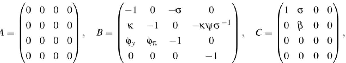
Thus, the above equations can represented as the regime switching system
A
cX
t−1c+ B
cX
tc+ qC
cX
t+1c+ (1
−q)CX
t+1= 0, (9) AX
t−1+ BX
t+ CX
t+1= 0, (10) with with X
t= (y
t,
πt, i
t, g
t)
0, and
A
c=
0 0 0 0 0 0 0 0 0 0 0 0 0 0 0 1
, B
c=
−1
0 0 1
κ −1
0
−κ ψ σ−10 0
−10
0 0 0
−1
, C
c=
1
σ0
−10
β0 0
0 0 0 0
0 0 0 0
,
A =
0 0 0 0 0 0 0 0 0 0 0 0 0 0 0 0
, B =
−1
0
−σ0
κ −1
0
−κ ψ σ−1 φy φπ −10
0 0 0
−1
, C =
1
σ0 0
0
β0 0
0 0 0 0
0 0 0 0
,
To solve system (9)-(10), we begin by solving (10) using Proposition 3 to find F such that
7A + BF + CF
2= 0.
Subsequently, define
A ˆ
c= A
c+ B
cµ+ qC
cµ2+ (1
−q)CF
µ, B ˆ
c= B
c+ qC
c2µ + (1
−q)CF, C ˆ
c= qC
c, and again invoke Proposition 3 to find the dominant solvent, S
c, of
A ˆ
cS
2c+ B ˆ
cS
c+ C ˆ
c= 0,
and uncover the solvent of (9) as F
c= S
−1c+
µ. Using the calibrated values of the parameters from Eggertsson (2011) reveals that F
cis the unique dominant solvent and given by
8F
c=
0 0 0 2.29 0 0 0 0.16
0 0 0 0
0 0 0 1
,
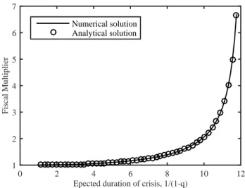
which suggests a fiscal multiplier of 2.29.
Figure 4 illustrates how the fiscal multiplier relates to the expected duration of the crisis, 1/(1
−q). As can be seen from the figure, the fiscal multiplier is moderate at short duration, and reaches arbitrarily large values as the duration approaches (approximately) 12 quarters. For values of q > 0.919 no solution can be found.
7Notice that in this particular example, the stable solutionFis simply a 4×4 matrix of zeros.
8The values are:σ=1/1.16,β=0.997,ψ=0.3664, andκ=0.0086. Stability is verified slightly differently in regime switching models, but in this particular case the eigenvalues of the “explosive solvent”multipliedbyqmust be greater than one (see Farmer, Waggoner and Zha (2009)).
Epected duration of crisis, 1/(1-q)
0 2 4 6 8 10 12
Fiscal Multiplier
1 2 3 4 5 6 7
Numerical solution Analytical solution
Figure 4: The relationship betweenqand the fiscal multiplier.
Notes.The multiplier increases exponentially inqand eventually reaches infinity. The analytical solution is obtained by evaluating equation (30) in Eggertsson (2011).
3.5 A large-scale problem
To explore the potential virtues of the proposed method for large-scale problems, I follow Higham and Kim (2000) and Tisseur (2000) and consider the n
×n quadratic matrix equation with
A =
15
−5−5
15
−5−5
. ..
. .. ...
. ..
−5−5
15
, B =
20
−10−10
30
−10−10
30
−10. .. . .. . ..
. .. 30
−10−10
20
,
and with C equal to the conformable identity matrix.
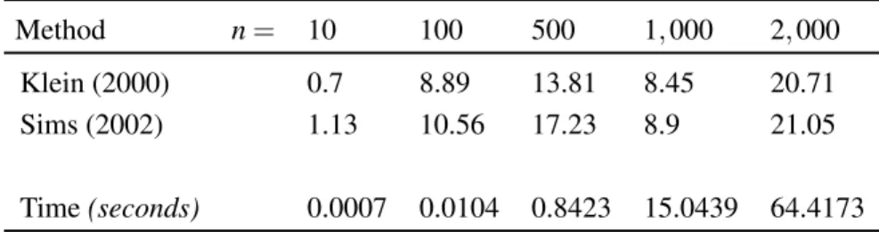
I then compare the execution time for using the iterations in both Propositions 1 and 2, and compare them with two popular alternative approaches by Klein (2000) and Sims (2002). The results are summarized in Table 1 below.
As can be seen from the table, the proposed method significantly outperforms both Klein’s
(2000) and Sims’s (2002) methods for n
≥100. In fact, the method is about 20 times faster for
very large-scale problems, such as n = 2, 000. Given that computing time falls from around 20
minutes to 1 minute for such problems, the proposed method appears to dominate existing methods
for problems as those in Reiter (2009).
Table 1: Speed comparison of algorithms.
Method n= 10 100 500 1,000 2,000
Klein (2000) 0.7 8.89 13.81 8.45 20.71
Sims (2002) 1.13 10.56 17.23 8.9 21.05
Time(seconds) 0.0007 0.0104 0.8423 15.0439 64.4173
Notes.The reported numbers in the two first rows represent the computational speed of the indicated algorithmrelative to that of time iteration. To make the comparison as fair as possible, I use the authors’ own codes. Computational speed is measured by the “timeit” function in Matlab, which evaluates a function several times and reports the median results.
The last line reports the time in seconds solving the problem using time iteration.
4 Concluding remarks
This paper has proposed a new approach to solve linear rational expectation models, and provided
conditions under which a stable solution can be ascertained to be unique. The main advantages of the
proposed method relative to existing methods is its transparency and ease of implementation without
relying on pre-canned routines, in addition to significant efficiency advantages for large-scale
problems.
A Proofs
A.1 Proof of Proposition 1
The recursion in (5) can be rewritten as
A+BFn+1+CFnFn+1=0.
Conjecture thatFnis given by
Fn= (S−(n−1)1 ΩSn2+S2)(S−n1 ΩSn2+I)−1.
Then,
FnFn+1= (S−(n−1)1 ΩSn2+S2)(S1−nΩS2n+I)−1(S−n1 ΩSn+12 +S2)(S−(n+1)1 ΩSn+12 +I)−1
= (S−(n−1)1 ΩSn2+S2)(S1−nΩS2n+I)−1(S−n1 ΩSn2+I)S2(S−(n+1)1 ΩSn+12 +I)−1
= (S−(n−1)1 ΩSn+12 +S22)(S−(n+1)1 ΩSn+12 +I)−1.
Inserting this expression into the recursion gives
A+B(S−n1 ΩSn+12 +S2)(S−(n+1)1 ΩSn+12 +I)−1+C(S−(n−1)1 ΩS2n+1+S22)(S−(n+1)1 ΩSn+12 +I)−1=Xn,
whereXnis an unknown. The left hand side of the above equation can alternatively be rewritten as A(S−(n+1)1 ΩS2n+1+I) +B(S1−nΩS2n+1+S2) +C(S−(n−1)1 ΩS2n+1+S22) =Xn(S−(n+1)1 ΩSn+12 +I).
SinceS2is a solvent it follows that
A(S−(n+1)1 ΩSn+12 +I) +B(S−n1 ΩSn+12 +S2) +C(S−(n−1)1 ΩSn+12 +S22)
=AS−(n+1)1 ΩSn+12 +BS−n1 ΩSn+12 +CS−(n−1)1 ΩSn+12
= (A+BS1+CS21)S−(n+1)1 ΩSn+12
=0,
where the second to last equality follows fromS1being a solvent. ThusXn=0 for alln. This confirms the conjecture.
By Lemma 1 we have that
n→∞limkS−n1 kkSn2k=0.
Thus,
n→∞limFn=lim
n→∞(S−(n−1)1 ΩSn2+S2)(S−n1 ΩS2n+I)−1=S2, Lastly, the initial valueF0is given by
F0= (S1Ω+S2)(Ω+I)−1.
SettingΩ6= (S1+I)−1−S−11 S2is necessary and sufficient to guarantee thatF06=S1, which completes the proof.
A.2 Proof of Proposition 2
The recursion in (6) can be rewritten as
AFˆnFˆn+1+BFˆn+1+C=0.
Conjecture that ˆFnis given by
Fˆn= (Sn2ΩS−n1 +I)(Sn+12 ΩS−n1 +S1)−1. Then,
FˆnFˆn+1= (Sn2ΩS−n1 +I)(Sn+12 ΩS−n1 +S1)−1(Sn+12 ΩS−(n+1)1 +I)(S2n+2ΩS−(n+1)1 +S1)−1
= (Sn2ΩS−n1 +I)(Sn+12 ΩS−n1 +S1)−1(Sn+12 ΩS−n1 +S1)S−11 (Sn+22 ΩS−(n+1)1 +S1)−1
= (Sn2ΩS−n1 +I)S−11 (Sn+22 ΩS−(n+1)1 +S1)−1.
Inserting this expression into the recursion gives
A(Sn2ΩS−n1 +I)S−11 (Sn+22 ΩS−(n+1)1 +S1)−1+B(Sn+12 ΩS−(n+1)1 +I)(S2n+2ΩS−(n+1)1 +S1)−1+C=Xn,
whereXnis an unknown. The left hand side of the above equation can alternatively be rewritten as
A(Sn2ΩS−n1 +I)S1−1+B(Sn+12 ΩS−(n+1)1 +I) +C(Sn+22 ΩS−(n+1)1 +S1) =Xn(Sn+22 ΩS−(n+1)1 +S1)−1.
SinceS1is a solvent it follows that
AS−11 +B+CS1= (A+BS1+CS21)S1−1=0.
Thus,
ASn2ΩS−n1 S−11 +BSn+12 ΩS−(n+1)1 +CSn+22 ΩS−(n+1)1 =Xn(Sn+22 ΩS1−(n+1)+S1)−1.
or
(A+BS2+CS22)Sn2ΩS−(n+1)1 =Xn(Sn+22 ΩS−(n+1)1 +S1)−1
=0, which confirms the conjecture. By Lemma 1 we have that
n→∞lim
Fˆn=lim
n→∞(Sn2ΩS−n1 +I)(Sn+12 ΩS−n1 +S1)−1=S−11 .
Lastly the initial value of ˆF0is given by
Fˆ0= (Ω+I)(S2Ω+S1)−1. SettingΩ=I, gives ˆF0=0, which completes the proof.
References
Binder, Michael and M. Hashem Pesaran, “Multivariate Rational Expectations Models and Macroeconometric Mod- elling: A Review and Some New Results,” in M. Hashem Pesaran and Michael R. Wickens, eds.,Handbook of Applied Econometrics: Macroeconomics, Oxford: Basil Blackwell, 1995, pp. 139–187.
Blanchard, Olivier and Charles M. Kahn, “The Solution of Linear Difference Models under Rational Expectations,”
Econometrica, 1980,48(5), 1305–1312.
Christiano, Lawrence J., “Solving Dynamic Equilibrium Models by a Method of Undetermined Coefficients,”Computa- tional Economics, 2002,20(1), 21–55.
Eggertsson, Gauti B., “What Fiscal Policy Is Effective at Zero Interest Rates?,” in Daron Acemoglu and Michael Woodford, eds.,NBER Macroeconomics Annual, Vol. 25 2011, pp. 59–112.
Farmer, Roger E.A., Daniel F. Waggoner, and Tao Zha, “Understanding Markov-switching rational expectations models,”
Journal of Economic Theory, 2009,144(5), 1849 – 1867.
Gohberg, I, P Lancaster, and L Rodman,Matrix Polynomials, New York: Academic, 1982.
Higham, Nicholas J. and Hyun-Min Kim, “Numerical Analysis of a Quadratic Matrix Equation,”IMA Journal of Numerical Analysis, 2000,20, 499–519.
King, Robert G. and Mark W. Watson, “System Reduction and Solution Algorithms for Singular Linear Difference Systems under Rational Expectations,”Computational Economics, 2002,20, 57–86.
Klein, Paul, “Using the generalized Schur form to solve a multivariate linear rational expectations model,”Journal of Economic Dynamics and Control, 2000,24(10), 1405–1423.
Reiter, Michael, “Solving heterogeneous-agent models by projection and perturbation,”Journal of Economic Dynamics and Control, 2009,33(3), 649–665.
Sims, Christopher A., “Solving Linear Rational Expectations Models,”Computational Economics, 2002,20(1), 1–20.
Tisseur, Francoise, “Backward error and condition of polynomial eigenvalue problems,” Linear Algebra and its Applications, 2000,309(1-3), 339–361.
Uhlig, Harald, “A Toolkit for Analysing Nonlinear Dynamic Stochastic Models Easily,” in Ramon Marimon and Andrew Scott, eds.,Computational Methods for the Study of Dynamic Economies, Oxford University Press, 2001.