ELECTROWEAK PRECISION PHYSICS FROM LEP TO LHC AND ILC

1

ELECTROWEAK PRECISION PHYSICS FROM LEP TO LHC AND ILC

W. HOLLIK

Max-Planck-Institut f¨ur Physik (Werner-Heisenberg-Institut) 80805 Munich, Germany

E-mail: hollik@mppmu.mpg.de

Eectroweak precision physics is reviewed from the LEP era with implications for Higgs bosons and supersymmetry, together with expectations for the LHC and a future Linear Collider ILC.

Keywords: Electroweak precision observables, standard model, Higgs bosons, supersym- metry

1. Introduction

High-precision experiments at electron-positron and hadron colliders together with the highly accurate measurements of the muon lifetime and gyromagnetic factor have imposed stringent tests on the standard model and possible extensions. The experimental accuracy in the electroweak observables is sensitive to the quantum effects and requires the highest standards on the theoretical side as well. A sizeable amount of theoretical work has contributed over the last two decades to a steadily rising improvement of the standard model predictions and also for specific new physics scenarios like supersymmetric extensions. Further improvements from are expected from the Tevatron and the LHC, and in particular from a future e

e

col- lider like the International Linear Collider (ILC) with an additional high-luminosity GigaZ option. The availability of both highly accurate measurements and theoret- ical predictions, at the level of 0.1% precision and better, provides unique tests of the quantum structure of the standard model and yields indirect informations on the Higgs mass as well as on potential other heavy new physics.

2. Electroweak Precision Observables

The possibility of performing precision tests is based on the formulation of the

standard model as a renormalizable quantum field theoriy preserving its predictive

power beyond tree-level calculations.

2.1. Muon decay and the vector-boson mass correlation

The basic physical quantity for the M

–M

correlation is the muon lifetime τ

, which defines the Fermi constant G

according to

1 τ

= G

m

192π

F

m

m

1 + 3

5 m

M

!

(1 + ∆

) , (1) with F(x) = 1 − 8x − 12x

ln x + 8x

− x

. By convention, the QED corrections within the Fermi Model, ∆

, are included in this defining equation for G

; they are known up to two-loop order,

∆

= 1 − 1.81 α(m

) π + 6.7

α(m

) π

, with α(m

) ≃ 1

135.90 . (2) From the precisely measured muon lifetime, the value

G

= (1.16637 ± 0.00001) · 10

GeV

for the Fermi constant is derived.

Calculating the muon lifetime within the standard model and comparing the result with (1) yields the relation

M

1 − M

M

= πα

√ 2G

(1 + ∆r) , (3)

where the radiative corrections are summarized in the quantity ∆r. Thereby, a set of infrared-divergent QED-correction graphs has to be removed, which reproduce the QED-correction factor of the Fermi-model result in (1). They have no influence on the relation between G

and the model parameters.

In the standard model the quantum correction ∆r has received a lot of atten- tion. The one-loop result

has been improved over the last two decades by complete QCD

and electroweak

two-loop terms as well as the leading 3- and 4-loop con- tributions,

establishing thus a powerful relation that can be used to predict M

within the SM (or possible extensions), to be confronted with the experimental re- sult for M

. The quantity ∆r depends on the entire set of input parameters. The photon vacuum polarization Π

(0) is a basic entry in the predictions for electroweak precision observables, resulting from the renormalization of the electric charge, or α, respectively. The difference

Re ˆ Π

(M

) = Re Π

(M

) − Π

(0) (4) is a finite quantity. The purely fermionic part corresponds to standard QED and does not depend on the details of the electroweak theory. It can be split into a leptonic and a hadronic contribution, yielding the quantity

∆α = ∆α

+ ∆α

= − Re ˆ Π

(M

) − Re ˆ Π

(M

) . (5) The leptonic content of ∆α can be directly evaluated in terms of the known lepton masses, yielding at three-loop order

∆α

= 314.97687 · 10

. (6)

3

classical limit. For the light hadronic part, perturbative QCD is not applicable and quark masses are no reasonable input parameters. Instead, the 5-flavour contribu- tion to ˆ Π

can be derived from experimental data with the help of a dispersion relation

∆α

= − α

3π M

Re Z

4m²π

ds

R

(s

)

s

(s

− M

− iε) (7) where

R

(s) = σ(e

e

→ γ

→ hadrons) σ(e

e

→ γ

→ µ

µ

)

is an experimental input quantity for the low energy range. Recent updates yield the value ∆α = 0.02758 ± 0.00035,

which is being used in the analysis of the precision data (see section 3).

2.2. Z boson observables

With M

used as a precise input parameter, together with α and G

, the predictions for the Z width, partial widths and asymmetries can conveniently be calculated in terms of effective neutral current coupling constants for the various fermions in the weak current (see e.g.

):

J

= √

2G

M

(g

γ

− g

γ

γ

) (8)

= √

2G

M

ρ

(I

− 2Q

s

)γ

− I

γ

γ

,

involving the effective (fermion-specific) mixing angles s

= sin

θ

. For the leptonic mixing angle, s

, the complete electroweak fermionic and bosonic two-loop contri- butions have become available

in the recent years, together with the universal terms of higher order mentioned already in the context of ∆r.

The effective mixing angles are of particular interest, since they determine the on-resonance asymmetries via the combinations

A

= 2g

g

(g

)

+ (g

)

, (9) namely

A

= 3

4 A

A

, A

= A

, A

= A

. (10) Measurements of the asymmetries hence are measurements of the ratios

g

/g

= 1 − 2Q

s

(11)

or the effective mixing angles, respectively.

2.3. Muon anomalous magnetic moment The anomalous magnetic moment of the muon, a

= g

− 2

2 (12)

provides a precision test at low energies. The new experimental result of E 821 at Brookhaven National Laboratory

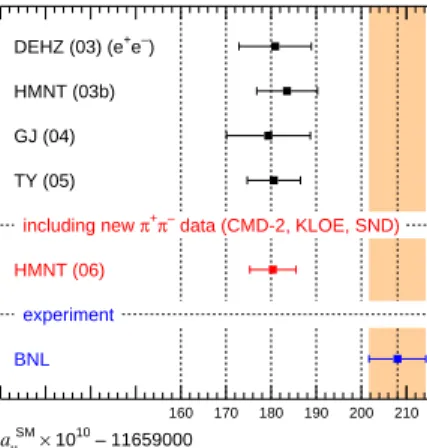
has reached a substantial improvement in accuracy. It shows a deviation from the standard model prediction by 3.4 standard deviations depending on the evaluation of the hadronic vacuum polarization from data based on e

e

annihilation

as shown in Figure 1. For a recent review see.

160 170 180 190 200 210

a_µ^SM × 10¹⁰ – 11659000 DEHZ (03) (e⁺e^–) HMNT (03b) GJ (04) TY (05)

including new π⁺π^– data (CMD-2, KLOE, SND) HMNT (06)

experiment BNL

Fig. 1. Measurements and standard model predictions foraµ= (gµ−2)/2.

3. Standard Model versus Data

The Z-boson observables form LEP 1 and SLC together with M

and the top-quark mass from LEP 2 and the Tevatron, constitute the set of high-energy quantities en- tering a global precision analysis (see

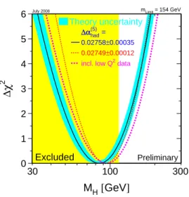
for a recent review). Global fits within the standard model to the electroweak precision data contain M

as the only free pa- rameter, yielding an upper limit to the Higgs mass at the 95% C.L. of M

< 154 GeV including the present theoretical uncertainties of the standard model predic- tions visualized as the blue band

in Figure 2. Taking into account the lower exclusion bound of 114 GeV for M

from the direct searches via renormalizing the probability shifts the 95% C.L. upper bound to 185 GeV.

The anomalous magnetic moment of the muon is practically independent of the Higgs boson mass; its inclusion in the fit hence does not change the bound on M

, but it reduces the goodness of the overall fit.

Theoretical bounds on the mass of the Higgs boson follow from the absence of

a Landau pole (upper bound) and from the requirement of a stable Higgs vacuum

5

0 1 2 3 4 5 6

100

30 300

M

[ GeV ]

∆χ

Excluded Preliminary

∆α_had =

∆α⁽⁵⁾

0.02758±0.00035 0.02749±0.00012 incl. low Q² data

Theory uncertainty

July 2008 m_Limit = 154 GeV

Fig. 2. χ²distribution for the Higgs boson mass from the electroweak global fit.

(lower bound). They are shown in Figure 3 as a function of the scale Λ up to which the standard model as a perturbative framework can be extrapolated.

As one can see, the allowed window for an extrapolation up to the Planck scale Λ = 10

GeV is consistent with the limits on M

obtained from direct searches and from indirect constraints via electroweak precision observables.

4. Perspectives for LHC and ILC

In the LHC era, further improved measurements of the standard model electroweak paramneters are expected, especially on the W mass and the mass of the top quark, as indicated in Table 1. The accuracy on the effective mixing angle, measureable from forward-backward asymmetries, will not exceed the one obtained already in

Fig. 3. Lower and upper Higgs boson mass bounds from vacuum stability and perturbativity versus the scale Λ up to which the standard model can be extrapolated.

e

e

collisions

. The detection of a Higgs boson would go along with a determi- nation of its mass with an uncertainty of about 100 MeV.

Table 1. Present and future experimental precision.

Error for now Tev/LHC LC GigaZ

MW [MeV] 33 15 15 7

sin²θeff 0.00017 0.00021 0.000013

mtop[GeV] 5.1 2 0.2 0.13

MHiggs[GeV] – 0.1 0.05 0.05

The ILC will improve the accuracy on M

substantially via scanning the e

e

→ W

W

threshold region.

The GigaZ option, a high luminosity Z factory, can provide in addition a significant reduction of the errors in the Z boson observables, in particular for sin

θ

≡ s

with an error being an order of magnitude smaller than the present one. Moreover, the top quark mass accuracy can also be considerably improved. The numbers are collected in Table 1.

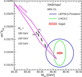
An ultimate precision test of the standard model that would be possible in the future scenario with GigaZ

is illustrated in Figure 4.

80.25 80.30 80.35 80.40 80.45 80.50 M_W [GeV]

0.23125 0.23150 0.23175 0.23200 0.23225 0.23250

sin2 θeff

presently

∆α m_t M_H =

180 GeV 150 GeV 120 GeV

SM@GigaZ 68% CL:

LEP/SLC/Tevatron LHC/LC GigaZ

Fig. 4. Prespectives for standard model precision tests at future colliders.

The figure displays the 68% C.L. regions for M

and sin

θ

≡ s

from the LHC and ILC/GigaZ measurements; the small quadrangles denote the standard model predictions for a possible, experimentally determined, Higgs boson mass with the sides reflecting the parametric uncertainties from ∆α and the top quark mass [for

∆α, a projected uncertainty of δ∆α = 5 · 10

is assumed]. If the standard model

is correct, the two areas with the theory prediction and the future experimental

results have to overlap.

7

5. Beyond the Standard Model: the MSSM 5.1. The Higgs sector

Among the extensions of the standard model, the minimal supersymmetric stan- dard model (MSSM) is the theoretically favoured scenario as the most predictive framework beyond the standard model. A light Higgs boson, as indicated in the analysis of the elctroweak precision data, would find a natural explanation by the structure of the Higgs potential.

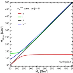
50 100 150 200 250 300 350 400 450 500 M_A [GeV]

50 100 150 200 250 300 350 400 450 500

MHiggs [GeV]

h H A H^+- m_h^max scen., tanβ = 5

FeynHiggs2.0

Fig. 5. Example of the Higgs boson mass spectrum in the MSSM.

The five physical Higgs particles of the MSSM consist of two CP -even neutral bosons h

, H

, a CP -odd A

boson, and a pair of charged Higgs particles H

. At tree level, their masses are determined by the A

boson mass, M

, and the ratio of the two vacuum expectation values, v

/v

= tan β. A typical example of a spectrum is shown in Figure 5. In particular the mass of the lightest Higgs boson h

is substantally influenced by loop contributions; for large M

, the h

particle behaves like the standard model Higgs boson, but its mass is dependent on basically all the parameters of the model and hence yields another potential precision observable. A definite prediction of the MSSM is thus the existence of a light Higgs boson with mass below ∼ 140 GeV. The detection of a light Higgs boson could be a significant hint for supersymmetry.

Present spectrum calculations comprise the complete one-loop terms and the

leading terms at two-loop order originating from the strong interaction and the t, b

Yukawa couplings (see e.g.

and references given there).

5.2. Precision observables

The structure of the MSSM as a renormalizable quantum field theory allows a simi- larly complete calculation of the electroweak precision observables as in the standard model in terms of one Higgs mass (usually taken as M

) and tan β, together with the set of SUSY soft-breaking parameters fixing the chargino/neutralino and scalar fermion sectors. The general discussion of renormalization of the MSSM to all orders with implications on the structure of the counter terms is given in.

Recent cal- culations for ∆r

and for the Z boson observables

are complete at the one-loop level and incorporate all available standard model two-loop and higher-order terms as well as the leading non-standard two-loop contributions

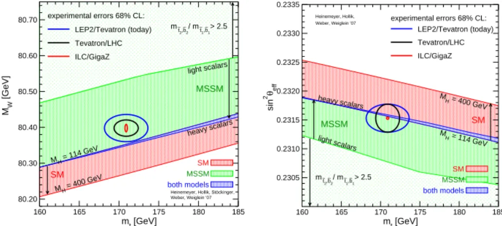
from the strong inter- action and the Yukawa couplings. A review on precision observables in the MSSM can be found in.

160 165 170 175 180 185

m_t [GeV]

80.20 80.30 80.40 80.50 80.60 80.70

MW [GeV]

SM

MSSM

MH = 114 GeV

MH = 400 GeV

light scalars

heavy scalars m_t

2

~,b~₂ / m_t

1

~,b~₁ > 2.5

SM MSSM both models

Heinemeyer, Hollik, Stöckinger, Weber, Weiglein ’07

experimental errors 68% CL:

LEP2/Tevatron (today) Tevatron/LHC ILC/GigaZ

160 165 170 175 180 185

m_t [GeV]

0.2305 0.2310 0.2315 0.2320 0.2325 0.2330 0.2335

sin2θeff

MSSM SM

M H = 400 GeV

M H = 114 GeV heavy scalars

light scalars

m_t

2

~,b~₂ / m_t

1

~,b~₁ > 2.5

SM MSSM both models

Heinemeyer, Hollik,

Weber, Weiglein ’07 experimental errors 68% CL:

LEP2/Tevatron (today) Tevatron/LHC ILC/GigaZ

Fig. 6. TheW mass and sin²θeff range in the standard model (lower band) and in the MSSM (upper band) respecting bounds are from the non-observation of Higgs bosons and SUSY particles.

As an example, Figure 6 displays the range of predictions for M

and sin

θ

in

the standard model and in the MSSM, together with the present experimental errors

and the expectations for the future collliders LHC and ILC/GigaZ. The MSSM

prediction is in slightly better agreement with the present data for M

, although

not conclusive as yet. Future increase in the experimental accuracy, however, will

become decisive for the separation between the models.

9

Especially for the muonic g − 2, the MSSM can significantly im- prove the agreement between theory and experiment: one-loop terms with relatively light scalar muons, muon-sneutrinos and charginos/neutralinos,

µ

γ

˜ µ χ_i

˜ νµ

˜ χ_i

µ

γ

˜ µ µa

˜ χ⁰_j

˜ µ_b

in the mass range 200 – 600 GeV, together with a large value of tan β can provide a positive contribution ∆a

, which can entirely explain the difference a

− a

(see

for a review).

The MSSM yields a comprehensive description of the precision data, in a similar way as the standard model does. Global fits, varying the MSSM parameters, have been performed to all electroweak precision data

showing that the description within the MSSM is slightly better than in the standard model. This is mainly due to the improved agreement for a

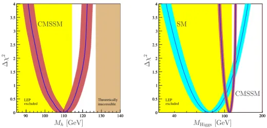
. The fits have been updated recently for the constrained MSSM (cMSSM), including also bounds from b → sγ and from the cosmic relic density. The χ

-distribution for the fit parameters can be shown

as a χ

-distribution for the lightest Higgs boson mass M

, displayed in Figure 7. The mass range M

= 110

GeV obtained from this fit is in much better agreement with the lower bound from the direct search than in the case of the standard model.

90 100 110 120 130 140

0 0.5 1 1.5 2 2.5 3 3.5 4

excluded LEP

inaccessible Theoretically

90 100 110 120 130 140

0 0.5 1 1.5 2 2.5 3 3.5 4

CMSSM

Mh[GeV]

∆χ2

40 100 200

0 0.5 1 1.5 2 2.5 3 3.5 4

excluded LEP

40 100 200

0 0.5 1 1.5 2 2.5 3 3.5 4

MHiggs[GeV]

∆χ2

CMSSM SM

Fig. 7. χ²-distribution for cMSSM fits, expressed in terms ofMh.

References

1. R.E. Behrends, R.J. Finkelstein, A. Sirlin, Phys. Rev.

, 866 (1956); S.M. Berman, Phys. Rev.

, 267 (1958); T. Kinoshita, A. Sirlin, Phys. Rev.

, 1652 (1959); T. van Ritbergen, R.G. Stuart, Phys. Rev. Lett.

, 488 (1999); Phys. Lett. B

, 343 (2000);

M. Steinhauser, T. Seidensticker, Phys. Lett. B

, 271 ((1999)

2. C. Amsler et al., et al. [Particle Data Group], Phys. Lett. B

, 1 (2008)

3. A. Sirlin, Phys. Rev. D

, 971 (1980); W.J. Marciano, A. Sirlin, Phys. Rev. D

, 2695 (1980)

4. B.A. Kniehl, Nucl. Phys. B

, 89 (1990); F. Halzen, B.A. Kniehl, Nucl. Phys. B

, 567 (1991); B.A. Kniehl, A. Sirlin, Nucl. Phys. B

, 141 (1992), Phys. Rev. D

, 883 (1993); A. Djouadi, P. Gambino, Phys. Rev. D

, 3499 (1994);

5. A. Freitas, W. Hollik, W. Walter, G. Weiglein, Phys. Lett. B

, 338 (2000); Nucl.

Phys. B

, 189 (2002); M. Awramik, M. Czakon, Phys. Rev. Lett.

, 241801 (2002);

Phys. Lett. B

, 48 (2003); A. Onishchenko, O. Veretin, Phys. Lett. B

, 111 (2003);

M. Awramik, M. Czakon, A. Onishchenko, O. Veretin, Phys. Rev. D

, 053004 (2003) 6. J. van der Bij, K. Chetyrkin, M. Faisst, G. Jikia, T. Seidensticker, Phys. Lett. B

, 156 (2001); M. Faisst, J. K¨ uhn, T. Seidensticker, O. Veretin, Nucl. Phys. B

, 649 (2003); Y. Schroder, M. Steinhauser, Phys. Lett. B

, 124 (2005); K. Chetyrkin, M. Faisst, J. K¨ uhn, P. Maierhofer, Phys. Rev. Lett.

, 102003 (2006); R. Boughezal, M. Czakon, Nucl. Phys. B

, 221 (2006); R. Boughezal, J.B. Tausk, J.J. van der Bij, Nucl. Phys. B

, 3 (2005);

, 278 (2005)

7. M. Steinhauser, Phys. Lett. B

, 158 (1998)

8. F. Jegerlehner, J. Phys. G

, 101 (2003); H. Burkhardt, B. Pietrzyk, Phys. Rev. D

, 057501

9. D. Bardin et al., hep-ph/9709229, CERN 95-03 (1995)

10. M. Awramik, M. Czakon, A. Freitas, G. Weiglein, Phys. Rev. Lett.

(2004) 201805;

M. Awramik, M. Czakon, A. Freitas, Phys. Lett. B

, 563 (2006); JHEP

, 048 (2006); W. Hollik, U. Meier, S. Uccirati, Nucl. Phys. B

, 213 (2005); B

,154 (2007); Phys. Lett. B

, 680 (2006)

11. H.N. Brown et al., Phys. Rev. Lett.

, 2227 (2001); G.W. Bennett et al., Phys. Rev.

Lett.

, 101804 (2002); Phys. Rev. Lett.

, 161802 (2004)

12. K. Hagiwara, A. Martin, D. Nomura, T. Teubner, Phys. Lett. B

, 173 (2007) 13. E. De Rafael, arXiv:08093085

14. The LEP Collaborations, the LEP Electroweak Working Group, the Tevatron Elec- troweak Working Group, the SLD Electroweak and Heavy Flavour Working Groups, LEPEWWG/2008-01, CERN-PH-EP/2008-020

15. T. Hambye, K. Riesselmann, Phys. Rev. D

, 7255 (1997) 16. S. Haywood et al., hep-ph/0003275, CERN 2000-004 (2000)

17. TESLA Technical Design Report, Part 3, J.A. Aguilar-Saavedra et al., hep-ph/0106315 18. J. Erler, S. Heinemeyer, W. Hollik, G. Weiglein, P.M. Zerwas, Phys. Lett. B

, 125

(2000); U. Baur et al., hep-ph/0111314

19. G. Degrassi, S. Heinemeyer, W. Hollik, P. Slavich, G. Weiglein, Eur. Phys. J. C

, 133 (2003)

20. W. Hollik, E. Kraus, M. Roth, C. Rupp, K. Sibold, D. St¨ ockinger, Nucl. Phys. B

, 3 (2002)

21. Heinemeyer, W. Hollik, D. St¨ ockinger, A.M. Weber, G. Weiglein, JHEP

, 052 (2006)

22. Heinemeyer, W. Hollik, A.M. Weber, G. Weiglein, JHEP

, 039 (2008)

23. A. Djouadi, P. Gambino, S. Heinemeyer, W. Hollik, C. J¨ unger, G. Weiglein, Phys.

Rev. Lett.

, 3626 (1997); Phys. Rev. D

, 4179 (1998); S. Heinemeyer, G. Weiglein,

11

JHEP

, 072 (2002);

24. S. Heinemeyer, W. Hollik, G. Weiglein, Phys. Rept.

, 265 (2006) 25. D. St¨ ockinger, J. Phys. G

, 45 (2007)

26. W. de Boer, A. Dabelstein, W. Hollik, W. M¨ osle, U. Schwickerath, Z. Phys. C

, 627 (1997); W. de Boer, C. Sander, Phys. Lett. B

, 276 (2004)

27. O. Buchmueller et al., Phys. Lett. B

, 87 (2007); JHEP

, 117 (2008)