Optical Spectroscopy of Spin Ladders

of

Spin Ladders

Inaugural - Dissertation

zur

Erlangung des Doktorgrades

der Mathematisch-Naturwissenschaftlichen Fakult¨ at der Universit¨ at zu K¨ oln

vorgelegt von

Marco Sascha Windt

aus Vechta (Niedersachsen)

K¨ oln, Dezember 2002

Berichterstatter: Prof. Dr. A. Freimuth

Priv.-Doz. Dr. G.S. Uhrig

Vorsitzender der Pr¨ ufungskommission: Prof. Dr. L. Bohat´ y

Tag der m¨ undlichen Pr¨ ufung: 14. Februar 2003

1 Introduction 3

2 Low-Dimensional Quantum Magnets 7

2.1 Some Basics . . . . 7

2.2 Antiferromagnetic Heisenberg Chains . . . . 12

2.2.1 Elementary Excitations . . . . 13

2.2.2 Alternating Chains and Spin-Peierls Transition . . . . 17

2.2.3 Doping of Chains . . . . 21

2.3 Ladders: Bridge between 1D and 2D . . . . 24

2.3.1 Even- and Odd-Leg Ladders . . . . 26

2.3.2 Interpretation of Susceptibility Data . . . . 29

2.3.3 Elementary Excitations: Triplets vs. Spinons . . . . 33

2.4 Telephone-Number Compounds . . . . 36

2.4.1 Crystal Structure of (Sr,La,Ca)

Cu

O

. . . . 36

2.4.2 Charge Carriers . . . . 40

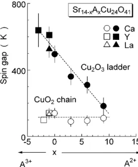
2.4.3 Spin Gaps . . . . 41

2.4.4 Superconductivity . . . . 44

2.4.5 Optical Studies . . . . 45

3 Optical Spectroscopy 51 3.1 Dielectric Function and its Determination . . . . 51

3.2 Typical Units . . . . 56

3.3 Bimagnon-Plus-Phonon Absorption . . . . 57

3.3.1 Experimental Evidence . . . . 57

3.3.2 Basic Idea . . . . 60

4 Experimental Setup 63 4.1 Fourier Spectroscopy . . . . 63

4.1.1 Calculating the Spectra . . . . 66

4.1.2 Problems to Take Care of . . . . 69

4.2 Sample Preparation . . . . 80

1

2 Contents

5 Bound States and Continuum in Undoped Ladders 87

5.1 First Predictions . . . . 87

5.2 Experimental Results . . . . 93

5.2.1 Reflectance . . . . 93

5.2.2 Transmittance . . . . 95

5.2.3 Optical Conductivity . . . 102

5.2.4 Subtraction of the Electronic Background . . . 107

5.3 Comparison with Calculations . . . 117

5.3.1 Jordan-Wigner Fermions and Continuous Unitary Transformations . 118 5.3.2 DMRG Results: Continuum and the Influence of a Cyclic Exchange 126 5.3.3 Resemblance to the S =1 Chain . . . 132

6 Doped Ladders 139 6.1 Sharp Raman Peak in Sr

Cu

O

. . . 140

6.2 Infrared Spectra of Sr

Cu

O

. . . 144

7 Conclusions 157

References 161

List of Publications 176

Acknowledgements 179

Abstract 180

Zusammenfassung 181

Introduction

Transition-metal oxides exhibit a vast panopticum of remarkable phenomena such as ordered states of spin, charge, and orbitals. These states along with the corresponding low-energy excitations are particularly interesting in low dimensions. For instance the unconventional superconductivity in the two-dimensional (2D) cuprates gave a special boost to the field of low-dimensional quantum magnets. The undoped parent compounds contain stacked layers of CuO

, which are supposed to be the best representations of 2D square-lattice Heisenberg antiferromagnets (AF) discovered so far. Since the spin of the involved Cu

ions is just 1/2 and since the number of neighbors on the square lattice is rather small, strong quantum fluctuations emerge that hinder long-range order.

These fluctuations most likely play an important role in explaining high-temperature superconductivity, that arises upon doping with charge carriers. Up to now, numerous ideas have been published but still no single theory can explain all the strange findings such as the linear temperature dependence of the resistivity in the normal state, the pseudo gap, or the origin of the pairing mechanism itself. Not even the exact ground state of the undoped 2D square-lattice Heisenberg AF with spin S = 1/2 is known so far.

However, analytical, semianalytical, and numerical techniques suggest AF long- range order with reduced staggered magnetization compared to the classical value. A comprehensive review on corresponding calculations is given in reference [1].

As a consequence of the difficulties in 2D, the quest for other materials containing one- and two-dimensional copper-oxide structures yielded a whole bunch of new magnetic features. 1D systems, for instance, provide a good testing ground to verify theoretical models that are exactly solvable. Moreover, numerical calculations on clusters with many sites can be counterchecked. To name but two examples, the spin-1/2 chain compound Sr

CuO

or the first inorganic spin-Peierls substance CuGeO

inspired much research ac- tivity. Even a step closer to the two-dimensional problem are spin ladders with a topology somewhere in-between 1D and 2D. By adding more and more chains to each ladder, the dimensional crossover can be approached. To stay within the ladder terminology, each chain gets labelled as a leg, accordingly with perpendicular rungs in-between (see fig- ure 1.1). Early calculations demonstrated that this crossover does not evolve smoothly.

Instead, the physics strongly depends on if there is an even or an odd number of legs involved [2].

1

The finite inter-layer coupling in the real materials induces long-range N´ eel order below an ordering temperature of typically 300 to 400 K.

3

4 Chapter 1 Introduction

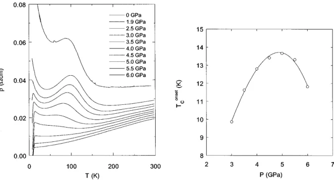
The theoretical study by Dagotto et al. published in 1992 predicted superconductivity in two-leg ladders upon doping with holes [3]. Two holes that are close-by show a tendency to occupy the same rung, which means that there is an attractive interaction. Sigrist et al. found that the order parameter exhibits d-wave-like symmetry, which resembles the high-T

cuprates [4]. After all, superconductivity was finally discovered in the doped two- leg ladder system Sr

Ca

Cu

O

by Uehara et al. in 1996 [5]. They applied high pressures of 3 and 4.5 GPa and found superconducting onset temperatures of 12 and 9 K, respectively. Yet it is not clear if the predicted mechanism is indeed responsible for the observed superconductivity. An alternative explanation is that the couplings simply get more two-dimensional under pressure.

Two-leg ladders with S = 1/2 exhibit a spin-liquid ground state with triplets as the elementary excitations. The triplet dispersion shows a gap [3], which is contrary to both 1D Heisenberg chains and odd-leg ladders that have gapless excitation spectra. The so- called telephone-number compounds (Sr,La,Ca)

Cu

O

provide excellent realizations of two-leg spin ladders, which are composed of the same corner-sharing plaquettes as the 2D cuprates. High-quality single crystals of various compositions are available, which were grown in mirror furnaces using the travelling-solvent-floating-zone method [6–8]. Apart from the ladder subcell, there is a second incommensurate subcell of spin chains. Holes doped into the compounds are expected to reside mainly in the chains [9], and charge ordering occurs within the chains of Sr

Ca

Cu

O

for x ≤ 5 [10].

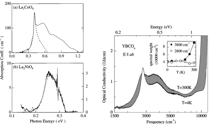
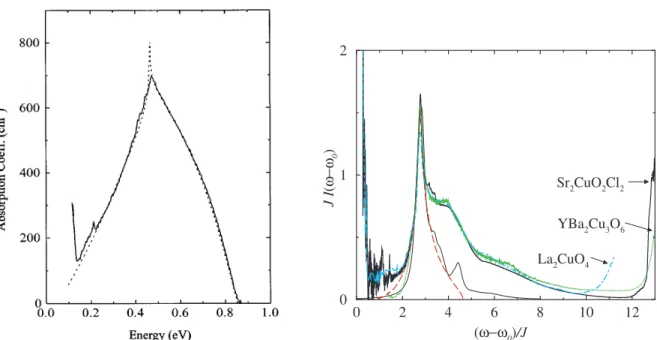
In general, infrared spectroscopy is one of the most popular spectroscopic techniques in solid-state physics. The breakthrough was the development of Fourier spectrometers, which provide many advantages over conventional dispersive spectrometers in the infrared range. By now, sophisticated devices are commercially available and can be found in many physics and chemistry labs. The use of infrared spectroscopy to study magnetic excitations proved already successful for the undoped 2D cuprates. The concept of phonon-assisted bimagnon absorption in combination with spin-wave theory [11, 12] is able to explain the sharp peak measured around 0.4 eV [13] in terms of an almost bound state of two magnons, which here is called a “bimagnon”. Yet there are additional sidebands at higher energies, which still cause a lot of discussion [14, 15]. In spin ladders we observe similar infrared spectra, i.e. two sharp peaks and a further high-energy contribution. Thus it is interesting to ask if there could be a real bound state in spin-ladder compounds.

For this quest of bound states in spin ladders, infrared spectroscopy is particularly suitable compared to other standard spectroscopic techniques. For instance the bound- state energies are quite high in cuprate ladders, which renders the quest for this state quite challenging by means of neutrons. Raman scattering is sensitive to excitations with vanishing total momentum, but the bound state only emerges at higher momenta. Infrared absorption is also restricted to k

= 0 excitations, but since the phonon participating in the phonon-assisted magnetic absorption provides momentum according to 0 = k

= k

+k

, it rather measures a weighted average of the magnetic spectrum over the whole Brillouin zone.

In fact, the complete magnetic infrared spectrum could unambiguously be explained

in cooperation with the theoretical groups of Uhrig et al. from the University of Cologne

and Kopp et al. from the University of Augsburg. The double peaks are indeed due to

a bound state of two triplets, whereas the sidebands could be identified with the multi-

triplet continuum. Such bound states in spin ladders have already been predicted before

Figure 1.1: Example of a small cluster of a two-leg ladder with 10 rungs. Con- trary to our experimental setup, this lad- der is illuminated by two separate light sources [28].

[16–23], but we were able to report the first experimental verification [24]. In addition to this remarkable result, the comparison of theory and experiment also yields the set of coupling constants along the legs and along the rungs. We could demonstrate that the inclusion of a four-spin cyclic exchange into the Hamiltonian is necessary to accurately reproduce the measured spectra and the spin-gap value determined by neutron scattering [25] at the same time [26].

The concept of binding is fundamental in physics [27]. Here, we discuss 1D quantum antiferromagnets, in which there are elementary excitations that carry a fractional spin of S = 1/2, the so called spinons. In most systems, spinons are not free but confined and form bound states with S = 1, i.e. triplets. The two-triplet bound state that we have identified in the infrared spectra thus can be viewed as a bound state of bound states.

To illustrate the phenomenon of binding one can draw a parallel to, for instance, the Coulomb interaction that binds electrons and atomic nuclei to form atoms.

Afterwards the interaction is mainly saturated, but there might still be some contribution left, that e.g. leads to the formation of higher-order bound states, namely molecules tied together by covalent bonds. The next hierarchy is then the formation of a solid by means of the van-der-Waals interaction. Other examples are for instance electrons and holes that bind to excitons and further on to biexcitons, or in the field of high-energy physics: quarks, hadrons, and nuclei.

Scope of this Thesis

The excitement surrounding ladder compounds was originally triggered by theoretical predictions of (i) the existence of a spin gap in the undoped phase and (ii) a transition to a superconducting state upon hole doping [3]. Both predictions have been sufficiently

2

Actually, the spin-spin interaction that leads to the formation of these magnetic bound states can be

traced back to the Coulomb interaction as well.

6 Chapter 1 Introduction

confirmed, and since 1992 a large amount of maybe 1000 papers on spin ladders has been published. However, many aspects are still not clear. In particular, no other analysis of the magnetic infrared spectra incorporating the mandatory transmittance measurements on thin samples has been reported so far to our knowledge.

In chapter 2 some basics on low-dimensional quantum magnets and their elementary excitations are discussed. After treating uniform and alternating Heisenberg chains, the Heisenberg ladders as a bridge between 1D and 2D are introduced. Afterwards the read- ers attention is turned to the telephone-number compounds (Sr,La,Ca)

Cu

O

, which represent the most widely studied series of spin ladders.

In optical spectroscopy we probe the linear response of solids to an applied electric field. This as well as the concept of phonon-assisted two-magnon absorption are briefly summarized in chapter 3, before in chapter 4 details on the experimental setup are pre- sented, which was put into operation within the framework of this thesis.

The infrared spectra of undoped telephone-number compounds are the subject of chap- ter 5. In comparison with theoretical results it is possible to unambiguously identify the signature of a bound state of two triplets and a multi-triplet continuum. The inclusion of a cyclic exchange in the analysis enhances the agreement between theory and experiment and reproduces the spin gap measured by neutron scattering. Thus the importance of this exchange term for a minimal model to describe spin ladders is verified. The analysis yields the complete set of the three relevant exchange couplings. The temperature dependence of the phonon-assisted magnetic absorption is discussed, and the relationship between the S = 1/2 two-leg ladder and the S = 1 chain is analyzed.

Chapter 6 deals with the effect of charge-carrier doping on the optical spectra. In

Sr

Cu

O

, charge ordering in the chain subsystem modulates the exchange coupling

along the ladders and thus leads to additional superstructure. Further mechanisms are

discussed that may explain some of the features in the doped compounds which are absent

in the undoped compounds of chapter 5.

Low-Dimensional Quantum Magnets

In the following, low-dimensional antiferromagnets (AF) and their elementary excitations are discussed. At first some basics are given, and then the attention is focussed on the 1D chain. Afterwards more detail on the current state of spin-ladder research is presented.

Finally, the “telephone-number” compounds are introduced, which take the center stage in this thesis.

2.1 Some Basics

The dimensionality of magnetic systems plays a crucial role when it comes to long-range ordering, phase transitions, spin gaps or low-energy excitations. At first there is the conventional dimension of the magnetic lattice d = 1, 2, 3, that corresponds to chains, planes, and 3D models. Below, notations like d = 2 and 2D are used as a synonym. But also the number n of spin components (x, y, z) has to be considered. The parameter n is called the spin dimensionality and is always to be distinguished from d. It is e.g. possible to have a 3D model with spin operators that just have one component along the z axis.

This would be the 3D Ising model with d = 3 and n = 1. For a given spin dimensionality n > 1 one may in addition vary the number of interacting spin components described by

Spin Dimensionality Interacting Components Name of Model J

= J

= J

Isotropic Heisenberg n = 3

J

= J

; J

= 0 XY S

= S

+ S

+ S

J

; J

= J

= 0 Z

n = 2 J

= J

Planar

S

= S

+ S

J

; J

= 0 Planar Ising n = 1

S

= S

J

Ising

Table 2.1: Classification of model systems. The different S

spin operators are given in the left column. Note that the magnetic lattice dimension is not specified. In fact, all the models may occur in 1, 2, or 3D. Based on references [29, 30].

7

8 Chapter 2 Low-Dimensional Quantum Magnets

Figure 2.1: Inverse correlation length along the chain axis for different d = 1 chain models versus a reduced tempera- ture T

. At high temperatures, all n = 3 models approach the isotropic Heisenberg limit. The calculations were performed within the classical spin formalism. Note that the classical Ising results are equal to the quantum-mechanical S = 1/2 case.

Reproduced from reference [30].

the exchange constants J

, J

, and J

, as illustrated in table 2.1. Of these models, the Ising, Heisenberg, and XY models are probably the most popular ones. But of course there are more possible combinations not listed in the table. For instance in three spin dimensions and for J

6= J

6= J

one gets the anisotropic Heisenberg or XYZ model.

To further illuminate this classification, one can e.g. have a look at the inverse corre- lation length (see figure 2.1) and discuss the difference between the XY and the planar model in 1D. In the XY model the interaction between the spins only has components within the xy plane, whereas the spins themselves are free to rotate in all three directions.

In the planar model, however, the spins are confined to the xy plane. At low temperatures the difference between the two models is not that significant. In the high-temperature limit the XY model approaches the 1D isotropic Heisenberg model. This is due to the thermal motion of the spins, which introduces a nonzero expectation value of the spin component along the z axis, even though J

= 0.

The isotropic Heisenberg model is often applicable to metal ions with open 3d shells.

In particular, it frequently describes systems with Cu

(S=1/2) or Mn

(S=5/2) ions rather well.

In all the models next-nearest-neighbor interactions are often neglected.

The reason is that in most considered materials the coupling is predominantly caused by superexchange, which is of extremely short range (J ∝ r

, n > 12) [32]. But the superexchange is also very sensitive to the actual bond angle. 180

bonds lead to strong AF exchange, whereas the exchange across 90

bonds is typically weak and ferromagnetic according to the Goodenough-Kanamori-Anderson (GKA) rules [33].

In three spatial dimensions (d = 3) most magnetic systems develop long-range order if only the temperature is sufficiently low. And this holds true independently from the spin

1

However, on the basis of ESR data it has recently been demonstrated that the exchange within 1D

CuO

chains is strongly anisotropic [31].

dimensionality. The case of n = 3 with just nearest-neighbor interactions can be described by the general Heisenberg Hamiltonian

H = X

i

J

S

S

+ J

S

S

+ J

S

S

. (2.1) Here again, S

, S

, and S

denote the components of the spin operator S = (S

, S

, S

), whereas J

, J

, and J

are the interactions for the different spin components, respectively.

In this convention, positive values of J are used for antiparallel coupling of neighboring spins, i.e. antiferromagnetic coupling, whereas J < 0 means ferromagnetic coupling. Prob- ably one of the best representations of a 3D Heisenberg antiferromagnet with spin S = 1/2 is KNiF

. This is a prototype system with 180

superexchange paths and a perovskite structure [34].

The spin itself is another crucial quantity that determines the system. Quantum- mechanically the spin is represented by operators with quantum numbers S = 1/2, 1, 3/2, 2, and so on. The crossover towards “classical” spin vectors is equal to S → ∞.

In this case the eigenvalue of the operator S

= S

+ S

+ S

, which is S(S + 1) ~

, can be replaced by S

~

. Quantum fluctuations disappear and the so-called N´ eel state becomes the ground state (see figure 2.2). In a bipartite lattice there are two sublattices A and B with, for instance, just spin-up and spin-down sites, respectively. In the absence of frustration there is AF interaction only between A and B spins. If there is any interaction within a sublattice, it is supposed to be ferromagnetic. Every deviation from this scenario is then called frustration. MnO is an example of N´ eel order in three dimensions with T

= 122 K [35]. As already mentioned above, the spin of the magnetic Mn

ion is S = 5/2 and thus substantially larger than the quantum limit of S = 1/2.

More generally, all states that show finite sublattice magnetizations hS

i − hS

i 6= 0 are labelled N´ eel states [36]. Therefore this definition also includes ferri magnets. Above the critical N´ eel temperature T

the order breaks down, and the system becomes para- magnetic. However, below T

one axis gets singled out even if there is no intrinsically favored direction within the crystal, which would be called an easy axis. This singled-out direction is not imposed externally, and such a phenomenon is called spontaneous symme- try breaking [27]. The Goldstone theorem states that in all cases with broken continuous symmetries there are excitations with arbitrarily low energy [37]. These excitations are called massless Goldstone bosons.

Figure 2.2: Classical N´ eel state in three di-

mensions of the magnetic lattice (d = 3). The

AF lattice of the magnetic ions is face-centered

cubic (fcc), whereas the corresponding paramag-

netic lattice is simple cubic (sc).

10 Chapter 2 Low-Dimensional Quantum Magnets

In 1D chains, on the other hand, there is no long range order above T = 0, regardless of the spin dimension. Only the Ising chain exhibits order right at zero temperature.

Whether there is an ordered state in two lattice dimensions depends on the symmetry of the Hamiltonian. The planar Ising model, for instance, orders at finite temperatures [38], whereas Mermin and Wagner proved in their classical letter [39] that for isotropic Heisenberg chains and planes with finite-range exchange interactions there cannot be spontaneous ordering at any finite temperature.

Thermal excitations disorder the spins already at infinitesimally low temperatures. Yet at T = 0 in the 2D square lattice the effect of zero-point quantum fluctuations is not strong enough [41], and thus the phase transition occurs exactly at zero temperature. Another example is the XY model in 2D.

Kosterlitz and Thouless showed that no long-range order of the conventional type exists [42]. Nevertheless, there is a state below a critical temperature T

that is characterized by a so-called topological order of spin vortices. Pairs of metastable vortices and antivor- tices are closely bound and eventually become free above the phase transition at T

. The mean magnetization is zero for all temperatures [43]. However, such a Kosterlitz-Thouless phase transition does not occur in the isotropic 2D Heisenberg model [42]. To sum up the occurrences of phase transitions at finite temperatures depending on the different spin and lattice dimensions, table 2.2 gives an overview of exemplary models for all combinations of d and n.

d = 1 d = 2 d = 3

Ising (n = 1) ◦ X X

XY (n = 2) ◦ KT X

Heisenberg (n = 3) ◦ ◦ X

Table 2.2: Presence ( X ) or absence (◦) of a transition to conventional long-range order of exemplary models at finite temperatures. The Kosterlitz-Thouless transition to topological order is denoted by (KT). Based on reference [29].

The thermodynamic behavior of magnets can be treated with mean-field (MF) theory, which is the simplest way to describe collective phenomena [44]. Nevertheless it has been successful to qualitatively describe magnetic phase transitions in 3D systems. For lower lattice dimensions, though, it appears to be inadequate since e.g. it predicts states of long-range order regardless of d. MF theory rather applies to classical magnets, and the actual critical temperatures T

always lack behind the calculated MF values of θ = zJ S(S+1)/3k

[29]. The parameter z is called magnetic coordination number and denotes the amount of nearest-neighbor spins. The discrepancy between T

and θ increases when spin fluctuations get more important. As a rule of thumb, these fluctuations become more important upon

(i) lowering the lattice dimension d, (ii) increasing the spin dimension n, (iii) reducing the involved spin values,

2

Essentially the same approach was used one year later by Hohenberg to exclude superfluidity at T > 0

in one and two dimensions [40].

(iv) decreasing the number of nearest-neighbor spins z, or finally (v) enhancing frustration.

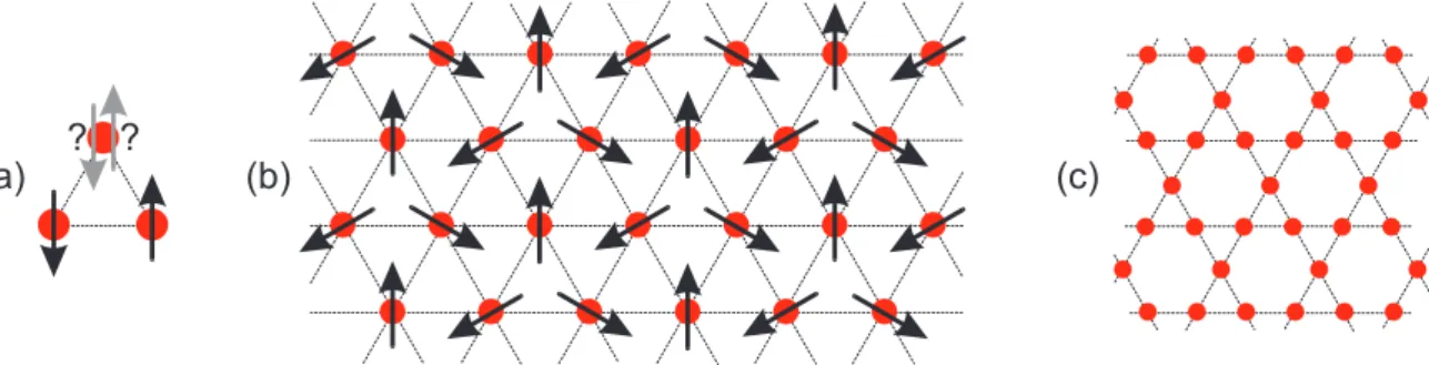
The last point is particularly obvious in a triangular plaquette as sketched in figure 2.3a.

There is no possible solution for the three neighboring spins to get aligned antiferromag- netically. However, the 2D triangular lattice indeed does exhibit long-range order. In the classical limit the ground state is a N´ eel state with the spins arranged at 120

to each other in three ferromagnetic sublattices (see figure 2.3b). But even in the quantum limit of S = 1/2 there probably exists an ordered N´ eel ground state with a sublattice magne- tization of as much as 50 to 60% of the classical value [45, 46]. The quite large magnetic coordination number of z = 6 helps to stabilize the system against extra fluctuations due to frustration. The situation is different for the Kagom´ e lattice with a lower value of z = 4 (figure 2.3c). Calculations indicate that there is no planar AF long-range order down to zero temperature [46, 47]. In general, such systems with no extensive magnetic order at T = 0 are called spin liquids. In analogy to real liquids there is, at the most, short-range order. The Kagom´ e system shows rather unusual properties, but the frustrated S=1/2 chain with antiferromagnetic exchange is an exemplary spin liquid. In AF chains frus- tration always emerges as soon as a further AF coupling between next-nearest-neighbor spins is present.

The notion of spin liquids was first proposed by Anderson. He also introduced the corresponding resonating valence bond (RVB) state that is contrary to the classical N´ eel state [48, 49]. In zeroth order the RVB model assumes a ground state consisting of nearest- neighbor singlet pairs. Higher-order corrections then allow the singlet pairs to move or

“resonate”, which makes this insulating singlet state more stable [49]. The actual state of the system is a linear superposition of such valence-bond singlets, corresponding to all possible pairings of sites into singlets with appropriate weight factors [50]. At this juncture it is sufficient to consider only bonds from one sublattice to the other. A simple visualization of such a product state in 1D is attempted in figure 2.4.

One of the main characteristics of RVB states is the absence of long-range order.

Therefore it is not surprising that the above mentioned factors that enhance spin fluctua- tions just as much favor the RVB state. For instance, rough estimates of the energies yield for the N´ eel case E

= −S

zJ/2 per spin and accordingly E

= −S(S + 1)J/2 for the

?

?

(a) (b) (c)

Figure 2.3: (a) Illustration of the no-win situation on a triangular plaquette with anti-

ferromagnetic coupling. This frustrated arrangement enhances spin fluctuations. (b) Nev-

ertheless, the triangular lattice does exhibit a N´ eel ground state with three ferromagnetic

sublattices. (c) An example of a spin liquid without long-range order is the Kagom´ e lattice.

12 Chapter 2 Low-Dimensional Quantum Magnets

Figure 2.4: Sketch of a possible RVB prod- uct state in 1D. The spin arrows might be mis- leading since in fact the singlets do not favor any direction.

RVB case [36]. Hence larger values of the spin coordination number z swiftly promote the classical limit. Increasing the spin has the same effect, though not as drastically. When the size of the superposed singlets in the RVB state stays finite, there will be a spin gap in the excitation spectrum. The gap energy then corresponds to the energy required to break up the “cheapest” singlet. However, in the case of infinitely large bonds also the N´ eel state can be described as a superposition of appropriate RVB states. With increasing bond length Monte Carlo simulations on the square lattice in reference [50] indicate disor- dered RVB states of very low energy. That shows that the RVB state gets competitive to a gapless N´ eel state with Goldstone excitations. Thus the difference between both types of states vanishes as soon as infinite-range singlets are included.

2.2 Antiferromagnetic Heisenberg Chains

From the above it becomes clear that the ground state of an antiferromagnetic 1D spin system is of exotic nature with quantum fluctuations impeding magnetic order. Theo- retical physics dealt with such systems since the early days of quantum mechanics as a simple model for many-body effects. The Hamiltonian of the Heisenberg spin chain can be written as

H = J X

i

(S

S

+ α S

S

) . (2.2)

The second term accounts for next-nearest-neighbor interactions. Therefore, with increas- ing the parameter α frustration gets enhanced. In the following, at first the frustration is switched off, i.e. α = 0. The classical ground state of the ferromagnetic case (J < 0) is simply the parallel alignment of all spins. However, in the AF case it is easy to demon- strate that the classical N´ eel state cannot be the ground state. With the help of raising and lowering operators

S

= S

± iS

(2.3)

the Hamiltonian 2.2 (still with α = 0) can be rewritten as H = J X

i

1

2 (S

S

+ S

S

) + S

S

. (2.4)

The mentioned classical ground state |ψ > would very well satisfy the spin-test relation

S

|ψ > = ±S|ψ > , (2.5)

but it is obvious that the inner bracket of Hamiltonian 2.4, applied to the N´ eel version of

|ψ >, transposes the spins of neighboring sites. Therefore the N´ eel state is not an exact eigenstate of the AF Hamiltonian.

Without frustration the model is exactly solvable, and the ground-state wave function of the Heisenberg chain with S = 1/2 was already determined by Bethe back in 1931 [51, 52]. Using Bethe’s solution it was Hulth´ en [53] who first calculated the exact ground- state energy eight years later for the AF case as

E

= −N (ln 2 − 1/4) . (2.6)

Explicit results for other physical quantities emerged slowly at first and only faster since around 1960. Of course interest in this model began to spread as soon as the first AF chain compounds became available. The total spin of the ground state is zero. Yet this state is somewhere in-between the N´ eel and the RVB state. The missing sublattice magnetization and the pronounced local singlet character of the wave function place it close to the RVB description. But as in the N´ eel state there is no excitation gap, and there are strong AF correlations since the decay follows a power-law [36].

As soon as frustration is allowed in the AF chain by increasing α, the RVB state gains ground in this contest. Many calculations were carried out for S = 1/2: In the case of α = 1/2, which is known as the Majumdar-Gosh point, the ground state is a dimer state consisting of a product of merely nearest-neighbor singlets [54–57]. It is two-fold degenerate and characterized by an excitation gap as well as the exponential decay of the spin correlation. In particular, the two-point correlation function < S

· S

> vanishes whenever |i − j| = 2, i.e. there is no correlation between adjacent singlets. The ground state energy amounts to E

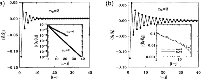
= −3/8J per spin as proven by van den Broek for infinite chains [58]. But there has to be a transition somewhere on the way from the gapless state at α = 0 to the pure RVB state with gap at α = 1/2. Numerical calculations yield rather precise values [59, 60]. At first, the excitation spectrum stays continuous but at the critical point of α = 0.24116(7) the energy gap finally emerges [60]. In section 5.3.3 more detail on the phase diagram of the chain is presented.

2.2.1 Elementary Excitations

Now the attention is turned to the excitations themselves. Before 1981, the excitations of S = 1/2 chains were generally assumed to be triplet spin-wave states with momentum k and spin S = 1 [61]. At least this was expected because of the situation in three- dimensional AF systems, where excitations are equal to delocalized spin flips with ∆S =

±1. However, Faddeev and Takhtajan introduced the spinon with spin S = 1/2 as the true elementary excitation in 1D [62].

Later, Haldane spoke of topological soliton excitations [64], since a spinon can be pictured as a movable domain wall within the chain, that separates two degenerate ground-state configurations. This image even works for N´ eel and RVB types of ground states. The N´ eel case is depicted in the top panel of figure 2.5.

3

It was already in 1979 that Andrei and Lowenstein discovered the spinon in a different context. They

diagonalized the Hamiltonian of the Gross-Neveu model and found excitations with spin 1/2 that only get

excited in pairs, and they called these excitations spinors [63]. The Heisenberg model was not mentioned,

but they used a modified Bethe ansatz which also holds true for the Heisenberg AF. All the spinon credit

is usually booked to Faddeev’s and Takhtajan’s account, though.

14 Chapter 2 Low-Dimensional Quantum Magnets

a)

b)

Figure 2.5: Representation of spinons as domain walls. The momentum of the sketched excitations is “k = π”. Panel (a) represents the N´ eel case, and panel (b) the RVB case. In contrast to figure 2.4 on page 12, here the misleading spin arrows within the RVB singlets are omitted. Note that spinons can only be excited in pairs.

The spin of 1/2 can be recognized especially in the RVB representation (figure 2.5b) due to the single unpaired spin. Both pictures are to be understood as oversimplifications, though. The RVB state for instance consists of singlets of different range, whereas the idealized N´ eel state does not exist anyway because of the fluctuations. Moreover, the spinon is not only the simple domain wall of figure 2.5, but it polarizes the environment.

This leads to some sort of polarization cloud [27].

Depending on if there is an even or odd number of spins, the total spin of the chain is either integer or half-odd integer. In chains with an odd number of sites there always has to exist at least one spinon. Actually, whether the total spin is integer or half-odd integer is a fundamental property of the system and cannot be changed by any excitation.

Although the spinon indeed is the elementary excitation, a single spinon would change the total spin by 1/2, and thus the excitation of a single spinon is not allowed. Instead, always two spinons are created simultaneously. In the N´ eel case it is easier to excite two spinons close to each other because all the spins in-between have to be flipped around.

And in the RVB state a singlet gets excited to a triplet, which directly yields two adjacent spinons.

Afterwards there is almost no confinement anymore that would tend to keep the spinons close-by. In fact, there is an interaction due to the polarization clouds, but the larger the distance between the spinons gets, the smaller the interaction is. This is meant by speaking of asymptotically free spinons.

Also important to note is that spinons cannot be gapless excitations in dimensions higher than one.

Domain walls are always objects of dimension d − 1 when the lattice dimension is d. But this means that the energy gets proportional to L

with L being the linear size of the system. Always when d ≥ 2, the energy exceeds all limits with increasing system size. This is not reasonable for elementary excitations [36].

The next step is to calculate the momentum or wave vector k of the spinons. For each eigenfunction |ψ > the quantum number k is defined by the relation

T |ψ > = e

|ψ > , (2.7)

where T is the operator that translates the entire chain by one lattice spacing [61]. To gain the dispersion of a single spinon one could for instance test the varying “ground-state

4

Of course this is only true for the pure RVB state. In case of long-range bonds the two spinons are separated right away.

5

Actually, this point is still under discussion. For instance Moessner and Sondhi claim that there are

gapped spinons in the 2D triangular lattice [65].

energies” of an odd-number chain with respect to different momenta. At this point, the naive picture of figure 2.5 for spinons as local domain walls breaks down. For values of k smaller than π the domain wall gets delocalized and sort of smears out. The corresponding wavelength of the spinon is λ = 2π/k. Therefore a state with vanishing momentum will occupy the whole length of the chain and the notion of a domain wall is obsolete. The first dispersion relation for the AF S = 1/2 chain was calculated by des Cloizeaux and Pearson [61], long before the spinons were invented. Their result was

E

(k) J = π

2 | sin(k)| . (2.8)

These spin-wave states are now understood to be a superposition of two spinons. The wave vector of two spinons is equal to the sum of both the single values k = k

+ k

. Thus there is always one free parameter when a double spinon with total momentum k is excited, and the real excitation spectrum will actually be a two-spinon continuum.

The lower boundary is given by the equation from above whereas the upper boundary corresponds to two spinons with:

E

(k)

J = π | sin(k/2)| . (2.9)

The continuum between lower boundary E

and upper boundary E

is marked as shaded area in the left panel of figure 2.6. By now, there are nice experimental verifications

0.0 0.5 1.0 1.5 2.0

0.0 0.5 1.0 1.5 2.0 2.5 3.0 3.5

Two-Spinon Continuum

Energy / J

Wave Vector k / π

1 2

ω 3 0 0.2 0.4 0.6 0.8 1 k / π 0

1 2

S

( k, ω )

Figure 2.6: Left panel: Two-spinon continuum as shaded area between the boundaries

of equations 2.8 and 2.9. The unit of the wave vector is in fact π/a, where a is the lattice

constant. But as usual, a is set to unity. Right panel: Exact result of the dynamical

structure factor S(k, ω) at T = 0 reproduced from reference [66]. Here ω denotes the

energy as is common in spectroscopy (see section 3.2). Again the continuum is marked as

shaded area. But contrary to the left panel only momenta up to k = π are shown. The

intensity plotted along the upright axis diverges at the lower boundary of the continuum

and approaches zero without any discontinuity at the upper boundary.

16 Chapter 2 Low-Dimensional Quantum Magnets

by means of inelastic neutron scattering, which is the experiment of choice to check dispersions. KCuF

for instance turned out to be an appropriate candidate for the S = 1/2 AF Heisenberg chain [67]. This compound shows 3D long-range order below T

≈ 39 K but exhibits almost ideal 1D chains above this temperature [68].

Measured scattering intensities are always weighted by the dynamical structure factor S(k, E), and especially in the case of continua it is not clear where to expect neutrons without model calculations.

Finally, Tennant et al. measured KCuF

[68, 70] and com- pared their intensities with calculations in the low-energy and zero-temperature limit by Schulz [71]. They measured along a line in the energy-momentum plane, as indicated in figure 2.7a, and found excellent agreement of their spectrum with the model data (figure 2.7b). As theoretical tools evolved further, the approximate structure factor used so far got replaced by exact results in 1997. The data of Karbach et al. [66] is shown in the right panel of figure 2.6. Again drawn as shaded area is the two-spinon continuum from the left panel, and the upright axis represents the dynamical structure factor. At the lower boundary the intensity diverges, whereas it approaches zero continuously at the upper boundary. The latter point actually marks the main difference compared to the older approximation which reveals a discontinuity at the upper boundary. But there is yet another interesting statement in the paper of Karbach et al. [66]. With the aid of sum rules it is possible to calculate that the two-spinon excitations account for approximately 73% of the total intensity in S(k, E). The rest of the overall spectral weight is due to excitations of more than two spinons. In the next section about spin-Peierls systems a nice experimental mapping of a complete spinon continuum is presented.

What happens in AF chains when the spin is larger than 1/2? One of the first points to clarify is the occurrence of a spin gap between the ground state and the first excited state. It was Haldane who used a semiclassical approach and predicted that Heisenberg chains with integer spins do exhibit energy gaps and thus are significantly different from half-odd-integer chains that show gapless excitation spectra [64]. The latter was already

6

In the case of inelastic neutron scattering the momentum and the energy of the incident neutrons are changed. The intensity I of neutrons with energy dE

that is scattered into the solid angle dΩ is directly proportional to the scattering cross section: I ∝

. This cross section again is proportional to the dynamical structure factor S

(k, E). Here, k and E mean the changes of momentum and energy in the scattering process and thus are equivalent to momentum and energy of the observed excitation. The parameters α and β denote the x, y and z components of the spin operator. In Heisenberg systems with no spin anisotropy the structure factor vanishes for all α 6= β . Often the structure factor is also called spectral density or scattering function. Finally, the intensity is related to the Fourier transform of the spin-spin correlation function < S

(t = 0) · S

(t) >. The stronger the correlation the more peak intensity can be expected. This can be deduced from the van Hove scattering function [69]. For simplicity, just contributions parallel to the z direction are considered, i.e. α = β = z

I ∝ d

σ

dΩ dE

∝ S

(k, E) ∝ X

R

Z

−∞

e

< S

(0) · S

(t) > dt . (2.10)

Neutron scattering hence measures directly the space-time Fourier transform of the (time-dependent) two- spin correlation function. Following the fluctuation-dissipation theorem, the structure factor furthermore is proportional to the imaginary part of the dynamical susceptibility χ

(k, E) times the Bose distribution

S

(k, E) ∝ χ

(k, E) 1

1 − e

. (2.11)

Figure 2.7: Neutron scattering data of KCuF

re- produced from reference [70]. (a) This continuum is equivalent to the one in the left panel of figure 2.6, though turned by 90

. The measurement was per- formed along the given line. Scattering intensity is observed when this line intersects with the continuum states as indicated by bold lines. (b) The result- ing three features at the corresponding energies can clearly be seen in the spectrum. The dashed line de- notes the fit to the background. The line shape is reproduced very well by the model fit using the cal- culated dynamical structure factor. The temperature was 20 K and thus it is interesting to note that the 1D quantum effects are dominant well below the 3D ordering temperature of T

≈ 39 K. Yet there is no drastic change up to 200 K except for the usual weak- ening and broadening of the features.

proven in reference [72]. Rigorous evidence for the meanwhile called Haldane gap was given later by Affleck et al. in reference [73]. As a consequence of a topological term in the field-theoretical formulation of the problem, the spinons are bound when the spin is integer. This leads to well defined, spin-wave-like modes that are separated from the ground state by the Haldane gap [70].

2.2.2 Alternating Chains and Spin-Peierls Transition

The model of the alternating Heisenberg chain is a straightforward generalization of the so far discussed uniform chain. Now the spin-spin interaction alternates between the two values J

and J

from bond to bond along the chain. In real systems this may be the consequence of the crystallographic structure such as different superexchange paths or just alternating distances between neighboring spin sites (see figure 2.8). The insulating magnetic salt (VO)

P

O

(VOPO) is an example [74, 75] although there was some con- fusion in early papers, where VOPO was mistaken for a spin-ladder compound.

Further candidates are CsV

O

[80] and the organic compounds (CH

)

CHNH

CuCl

[81] as well as Cu

(C

H

N

)

Cl

[82]. But again, it is difficult to extract the correct magnetic config- uration from the available data. For example, the calculated susceptibilities of different

7

VOPO (vanadyl pyrophosphate) has been widely considered to be a candidate for a two-leg AF

Heisenberg spin ladder with legs running along the a axis [76–78]. However, more recent results from

inelastic neutron scattering on powder samples [79] were inconsistent with the ladder model. Finally,

neutron data on single crystals published somewhat later [74] verified that VOPO is instead an AF

Heisenberg chain system with alternating couplings along the b axis. Thus the chains run perpendicular

to the assumed ladders. The magnetic V

ions have spin 1/2, and there is weak ferromagnetic interchain

coupling. In general, it is difficult to distinguish between the two models from static susceptibility or

neutron data of powder samples.

18 Chapter 2 Low-Dimensional Quantum Magnets

J ₁ J ₂

Figure 2.8: Example of an alternat- ing chain. The interaction J

within a dimer is stronger than the interaction J

between the dimers. The lattice spac- ing is doubled compared to the uniform chain.

spin models often agree that much that all of them reproduce the experimental data better than the agreement between different measurements of the same compound [82].

Accurate calculations of the magnetic susceptibility and of the specific heat for different systems were given by Johnston et al. [83].

The new magnetic Hamiltonian has reduced translational symmetry due to the dimer- ization, and just including nearest-neighbor interactions it reads as follows

H =

N/2

X

i=1

(J

S

S

+ J

S

S

) . (2.12)

It is common to define an inter-dimer coupling parameter λ = J

/J

with 0 ≤ λ ≤ 1.

In the case of unity one simply gets the isotropic chain with gapless excitations, and for vanishing λ the system is reduced to uncoupled dimers. Then a gap occurs which is equivalent to the breakup of a single dimer

and thus E

= J

. In-between there is the regime of coupled AF dimers in a singlet S = 0 ground state with a gap to the lowest S = 1 triplet excitation. A continuum of excitations sets in at 2E

. Both the triplet gap and the continuum edge were observed in CuGeO

by means of inelastic neutron scattering [84] (see below). Analytical results can be derived using perturbation theory about the isolated dimer limit, i.e. λ = 0. But real systems often are closer to the critical point of the uniform chain. VOPO for instance has a value of λ = 0.8 [74]. And copper germanate (CuGeO

), which is discussed below, exhibits an λ around 0.95 [85, 86].

Another approach is to distort the uniform chain in terms of the distortion parameter δ =

. With the average value of ˜ J =

the alternating couplings become

J

= ˜ J(1 + δ) and J

= ˜ J(1 − δ) . (2.13) Finally, the Hamiltonian 2.12 can be rewritten as

H = ˜ J X

i

(1 + (−1)

δ) S

S

. (2.14)

Cross et al. [87] as well as Black et al. [88] discuss such weak dimerization and following their approach, which involves a Jordan-Wigner transformation

, the gap energy is

lim

E

J ˜ ∝ δ

p | ln δ| . (2.15)

8

The Hamiltonian of a single dimer reads H = J S

S

=

(S

+ S

)

−

. Therefore one finds a singlet energy of E

= −3J/4 and a triplet energy of E

= E

+ J = 1/4J .

9

The Jordan-Wigner transformation [89] allows to map a one-dimensional S = 1/2 system exactly

onto interacting fermions without spin.

Figure 2.9: Spinon dispersion of an alternating chain for different inter- dimer couplings λ = J

/J

[91]. Note that in the figure α is equal to λ. When comparing the result of the uniform chain at λ = 1 with the former spinon dispersion on page 15, one has to keep in mind that here the lattice spacing b is doubled. Therefore the dispersion for the uniform chain given here is equal to the first arc of the lower boundary of figure 2.6(left). Again, the energy is denoted by E = ~ ω with ~ set to unity.

Contrary to the intrinsically dimerized compounds described so far, alternating chains may also arise as a result of the spin-Peierls effect. In this case the spin chains are not isolated anymore but instead a coupling to the phonons of the complete lattice has to be included. A spatial dimerization of the ionic positions along the chain yields alternating interaction strengths and results in the lowering of the magnetic ground state energy.

But as usual this advantage has to be paid for by an increase of lattice energy. The corresponding phonon contribution to the energy dominates at large distortions. An equilibrium will be reached at the lowest possible ground state energy. The spontaneous dimerization that occurs with decreasing temperature at T

is known as the spin-Peierls effect. In fact, a second-order phase transition occurs at T

. And since the lattice instability is driven by magnetic interactions, this transition is called magneto-elastic.

The resulting magnetic Hamiltonian is equal to the given alternating chain Hamiltonian (equation 2.12 or 2.14). But when the temperature is decreased even further, a new equilibrium will be adopted and the dimerization gets stronger. Therefore λ becomes inherently temperature dependent.

The first inorganic example of a spin-Peierls compound is CuGeO

, which was discov- ered in 1993 [90]. The crystals are light blue, similar to “Wick Blau” r , the German brand of Vicks cough drops. So far no other inorganic system has been proven to exhibit a spontaneous dimerization. The transition occurs at T

= 14 K, and below this tempera- ture the magnetic susceptibility rapidly drops for all three directions to small constant values. However, the role of competing next-nearest-neighbor (NNN) interactions was discussed as an extension of the model in order to explain the susceptibility data. The frustration has the effect of increasing the transition temperature [85]. The admixture of NNN coupling was estimated to be somewhere between 0.24 and 0.36 [85, 86] and thus possibly beyond the critical value of 0.2412 at which a gap would occur even without dimerization (see page 13).

Dispersion relations of the magnetic excitations were presented in reference [91, 92].

The calculations were based on a combination of the Lanczos algorithm and multiple-

precision numerical diagonalization to determine perturbation series to high order. In

figure 2.9 the result is shown for a number of different inter-dimer couplings λ = J

/J

.

Of course, the λ = 1 dispersion has to be equivalent to the uniform-chain result. The

20 Chapter 2 Low-Dimensional Quantum Magnets

(d) (c) (b) (a)

Figure 2.10: Spinon confinement. (a) Excitation of a local triplet. (b) The two spins can move away from each other at the cost of building weakly coupled dimers in-between.

Two spinons are formed. (c) The potential energy rises further the more weak dimers are formed. (d) For large distances it is energetically favorable to create another pair of spinons compared to a situation with a large number of weak dimers. The total spin of the excitation is still S = 1. Based on reference [27].

dimer limit of λ = 0 yields just a straight line with an energy gap of J

. Without dispersion the excitation cannot move along the chain, and thus the excited triplet stays localized. By switching on the coupling between the dimers, which means increasing λ, the gap energy gets smaller. At the same time the excitation can hop as a whole from dimer to dimer, and the bandwidth of the dispersion increases. Both the spins that form the triplet can also separate, and we get two spinons. But there is an important difference to the asymptotically free spinons of the uniform chain. The corresponding mechanism is illustrated in figure 2.10: As soon as the spinons move away from each other, new singlet dimers are formed in-between. But the coupling is weaker because the spin sites are further apart compared to the initial dimers. In terms of energy this configuration is unfavorable, and the situation gets worse the more weak dimers are formed. Hence the energy increases with distance d, and there is a potential V (d) that tries to keep the spinons nearby. The spinons are bound, and their movement is hampered by this new confinement. From a certain distance on it gets “cheaper” to excite a new pair of spinons than to build further weak dimers. Energetically this corresponds to 2E

, where the energy is sufficient to excite two triplets.

A dimerization of the chain thus binds spinons to pairs [17, 93]. The total spin of such a bound spinon is either S = 0 for a singlet or S = 1 for a triplet. These two types of excitations both yield a well defined excitation branch. The energy of the triplet is lower than the singlet energy. Strictly speaking, the spinons are not the elementary excitations anymore due to the binding. Instead the triplet spinon pairs get labelled to be the new elementary excitations. This appears naturally from the point of view of isolated dimers discussed above.

Both branches are located below the continuum, that still is present in the dimerized

chain. The continuum has to emerge from two unbound excitations, which can be regarded

as either two triplets, two spinons, or two pairs of spinons. Due to spin-rotation symmetry

the gap of the continuum is twice the elementary triplet gap [17]. But there is also another

0 1 2

0 .0 0 .5 1 .0

k ( π ) 0

1 2

(a ) 3

C o n t i n u u m

ω ( J )

S = 0 (b )

k = π

2 ∆ 2 ∆

∆

∆

S ( ω )

ω ( J )

S=1

S=0, 1, 2

Figure 2.11: Sketch of the dispersion and the spectral density of the dimerized chain, reproduced from reference [27]. (a) The bottom curve shows the elementary branch of the triplet. Just above is the singlet branch. The shape of the continuum can be derived from the spinon continuum of the uniform chain (see page 15) or by taking all possible combinations of two triplets. The dashed line is a guide to the eye to indicate the “uniform”

continuum (right area), although now with a gap. Due to the doubling of the unit cell the Brillouin zone is cut in half at k = π/2. Hence the “right” continuum is mirrored or folded back along the k = π/2 line, and the “left” area emerges. The complete continuum is the combined area of both contributions. When the dimerization is weak there won’t be much intensity from the “left” area. ∆ and 2∆ denote the gaps to the elementary triplet and to the continuum, respectively. (b) Structure factor or spectral density at momentum k = π.

Of course, with neutrons only S = 1 excitations are accessible.

way of interpreting the singlet branch. If one prefers to choose the triplet picture without the concept of spinons, at least two triplets have to be excited to yield a singlet state.

This would be a bound state of two triplets with antiparallel alignment.

The excitation spectrum of the alternating chain with the two branches of bound states and the continuum is sketched in the left panel of figure 2.11. The right panel illustrates the spectral densities at momentum k = π with two sharp peaks stemming from the bound states. The triplet peak and the continuum of CuGeO

were measured with neutrons [84], as discussed above. The continuum had already been mapped before by Arai et al. [94].

Their impressive plot is presented in figure 2.12. However, the resolution had not yet been high enough to see the triplet bound state. And since dimerization is low in CuGeO

the continuum resembles the one of the uniform chain, but of course the spin gap is present.

With neutrons it is not possible to measure S = 0 singlet excitations. Such excitations at momentum k = 0 are accessible by inelastic Raman scattering [95–97]. In Figure 2.13 the Raman spectrum of CuGeO

is plotted. The sharp peak is clearly visible but not separated from the weak continuum that follows.

2.2.3 Doping of Chains

So far, no doping of charge carriers or magnetic impurities has been discussed. The

simplest possibility is to replace some spins by spinless impurities, such as it occurs by

doping with Zn

ions. The effect is quite similar for a variety of different spin models

and is caused mainly by short-distance physics. A small percentage of vacancies rapidly

22 Chapter 2 Low-Dimensional Quantum Magnets

Figure 2.12: Map of the dynamical struc- ture factor of CuGeO

, measured with inelastic neutron scattering at 10 K by Arai et al. [94].

The dimerization in CuGeO

is quite small and thus the left “mirror” intensity of figure 2.11 is not present. Therefore the continuum resem- bles the spinon continuum of the uniform chain.

The arcs of the lower boundary are very dis- tinct. Since these arcs do not reach all the way down to zero energy the gap is verified. Also the upper boundary of the continuum is accord- ing to expectations. Due to the resolution of the measurement the triplet bound state is not separated from the continuum but was verified later in reference [84].

destroys spin gaps, and their presence induces enhanced AF correlations nearby [98, 99].

Again, CuGeO

is a fruitful example [100–103]. The explanation acts on the assumption of localized spinons near the doped vacancies that interact with each other through weak effective AF couplings. This interaction will get stronger the more Zn is doped into the system. Calculations demonstrated that these localized states form a low energy band in the spectrum, which appears inside the original spin gap of dimerized chains and also of the spin ladders discussed in the next section [104].

Charge-Carrier Doping

Much effort has been spent to describe the copper-oxide planes of superconducting cuprates which are doped with holes. Fortunately, the concepts can often be applied to other Cu-O systems as well. Let us start from the undoped case. The Cu

ion pos- sesses nine electrons in the 3d shell. The degeneracy of the 3d orbitals is lifted by the crystal field, resulting in a single hole in the d

orbital. This leads to a half-filled band

Figure 2.13: Raman spectrum of CuGeO

repro- duced from figure 1 of reference [97], yet simplified and rearranged. Inelastic photon scattering is sensitive to S = 0 excitations. Thus the sharp peak arises from the singlet bound state. The subsequent continuum is not separated from this peak, though.

10 20 30 40 50 T=2.2K

Intensity (a.u.)

Energy Shift (cm

)

of d

orbitals within the crystal. Accordingly, band structure calculations predicted a non-magnetic metallic state [105], which is in clear contrast to the insulating gap of the order of 1.5 eV observed in optical spectra [106–108]. This failure of band theory is due to the large on-site Coulomb repulsion U that forces the electrons to avoid double occupancy of a single orbital. In this situation the electrons are strongly correlated.

When further holes get doped into copper-oxide spin systems, effective Cu

ions are created with spin S = 0. In fact, no real Cu

ions occur but instead hybridization be- tween copper and oxygen strongly binds a hole to a central Cu

ion and its surrounding oxygen ions. This leads to the formation of a local singlet which is well-known as the Zhang-Rice singlet [109]. Overlap between neighboring sites allows for hopping of elec- trons and thus the singlet can move. The Zhang-Rice singlet corresponds to a spinless fermion moving in the background of Cu spins without doubly occupied sites. It repre- sents an empty site or hole, respectively, in the copper lattice. The kinetics of holes in the background of an S = 1/2 Heisenberg AF can be described by the t–J model, which is an effective low-energy model for single or multi-band Hubbard models. The parameter t denotes the site-hopping matrix element. The AF exchange is then given by

J = 4t

/U (2.16)

with U being the already mentioned on-site Coulomb repulsion. In the t–J approach this repulsion is assumed to be larger than the hopping: U t. At exactly half filling of the band the charge excitations are gapped, and the low-energy degrees of freedom are purely magnetic. In this case the t–J model reduces to the standard Heisenberg model.

In 2D the Hubbard model as well as the t–J model have not been solved exactly, and not even the ground states are entirely known so far. A lot of numerical calculations on finite clusters were performed, but the complexity grows outrageously with cluster size.

The computation of a 32-site cluster within the t–J model already requires to handle ma- trices with dimensions of up to 3 × 10

[110]. That is the reason why the probing question whether there is superconductivity in these models has not been answered satisfactorily to date.

In 1D, however, the low-energy properties of many gapless quantum systems can be described by the exactly solvable Luttinger model [111]. The class of models that can be mapped onto so-called Luttinger liquids includes the 1D Hubbard model away from half-filling and thus also the 1D t–J model. One of the key properties is the spin-charge separation: instead of quasiparticles like in Fermi liquids, collective excitations of charge (with no spin) and spin (with no charge) are formed, that move independently and even at different velocities. Just recently our group found evidence for this phenomenon in the Bechgaard salts by measuring the electrical and thermal conductivity [112].

Another interesting effect is the occurrence of charge ordering in doped chains.

Sr

Cu

O

for instance is inherently doped with charge carriers. The nominal hole count

yields six holes per formula unit, and the holes are expected to reside mainly within the

sublattice of the CuO

chains. N¨ ucker et al. estimated the distribution of holes at room

temperature via x-ray absorption spectroscopy [9]. They found approximately 5.2 holes in

the chains, whereas 0.8 holes are located within the other sublattice, which includes layers

of spin ladders. This telephone-number compound will be discussed in greater detail later

on. Below the temperature of approximately 200 K a superstructure occurs due to charge

ordering in the chains. Regnault et al. used inelastic neutron scattering and proposed a

24 Chapter 2 Low-Dimensional Quantum Magnets

Cu O

Figure 2.14: The charge ordering in the chains of Sr

Cu

O

produces a superstructure with the periodicity of five lattice spacings. The squares denote Zhang-Rice singlets.

model of interacting AF dimers with intra- and interdimer distances equal to 2 and ≈ 3 times the distance between neighboring copper ions [113]. This implies that almost no charge carriers are left within the ladders at low temperatures. A possible illustration of such an arrangement is sketched in figure 2.14. The holes are drawn as squares to symbolize Zhang-Rice singlets. AF dimers are formed between spins that are separated by a single hole. The dimers are separated by two holes from each other, which leads to only weak magnetic exchange. The charge order in Sr

Cu

O

is discussed in greater detail in chapter 6.

2.3 Ladders: Bridge between 1D and 2D

The humble survey of 1D chains demonstrated that a great deal of the rich phenomena are understood after a long period of research. The important models are solved and experiments support the theoretical results. The 2D square-lattice Heisenberg AF is far from this state. Some hope is associated with the ladders that topologically are situated between one and two dimensions. One can start with a single chain, or leg, and successively couple further chains to it, until finally the square lattice is approached. Neither in Heisenberg chains, nor in the 2D square-lattice there is a spin gap for S = 1/2. The corresponding ground states are of spin-liquid and AF type, respectively. And of course it is very instructive to examine what happens in-between, both in theory and experiment.

This section is chiefly based on the comprehensive reviews on ladders presented in reference [2] by Dagotto and Rice, and in reference [114] by Dagotto.

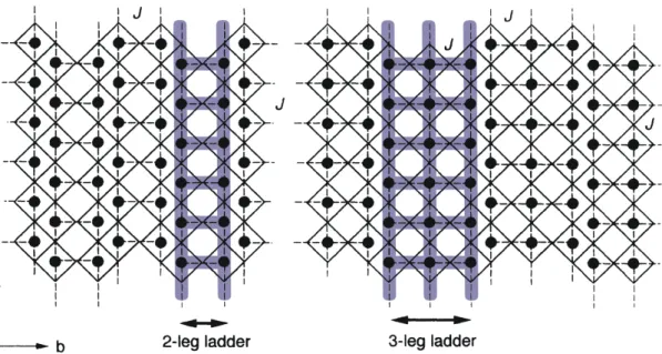
AF Heisenberg ladders with two and three legs, respectively, are sketched in figure 2.15. The exchange coupling along the legs is labelled as J

, and J

denotes the rung coupling. The Hamiltonian of the simplest case with just two legs reads

H = X

i

{ J

(S

S

+ S

S

) + J

S

S

} . (2.17)

The first two terms represent the interaction between neighboring spins along the two

legs, and the last term takes care of the interaction within each rung. The first index of

each spin operator denotes the leg number, whereas the second index counts the rungs

(confer top panel of figure 2.15). Reference [3] might be regarded as the starting point

of the recent interest in ladder physics. The early calculations on two-leg ladders with

J

J

, usually called the strong-coupling limit, found a finite spin gap. This came as

a surprise since the limiting cases of 1D chains and 2D planes are both gapless, yet it

is easy to comprehend in the strong-coupling limit. Here the rungs interact only weakly