Disentangling and machine learning the 
 many-fermion problem

Disentangling and machine learning the 
 many-fermion problem

Peter Bröcker

Dissertation

Disentangling and machine learning the many-fermion problem

Inaugural-Disserta8on

zur


Erlangung des Doktorgrades


der Mathema4sch-Naturwissenscha:lichen Fakultät der Universität zu Köln


vorgelegt von

Peter Bröcker geb. Boertz aus Münster

Köln, 2018

Prof. Dr. David Gross

Tag der mündlichen Prüfung: 16.4.2018

Contents

I. Monte Carlo methods for the many-body problem 7

1. The Monte Carlo method 8

1.1. Fundamentals of the Monte Carlo method in physics . . . . 8

1.1.1. Markov chains . . . . 8

1.1.2. Moving along Markov chains . . . . 9

1.2. Analysis of Monte Carlo data . . . 10

1.2.1. Calculating mean values and their error bars . . . 10

1.2.2. Autocorrelation . . . 11

1.2.3. Functions of observables . . . 12

2. Determinant Quantum Monte Carlo 13 2.1. Theoretical formulation . . . 13

2.1.1. Finite temperature simulations . . . 15

2.1.2. Projective formulation . . . 17

2.2. The Hubbard-Stratonovich transformation . . . 18

2.3. Numerical implementation . . . 21

3. Stochastic Series Expansion 25 3.1. Formulation of the Monte Carlo procedure . . . 25

3.2. Sampling operator sequences . . . 26

3.3. Measurements . . . 30

4. The sign problem 31 4.1. Monte Carlo calculations with sign problem . . . 31

4.2. The physical origin of the sign problem . . . 32

4.3. Circumventing the sign problem . . . 33

II. Disentangling and learning 35 5. Entanglement 36 5.1. Entanglement and its use in condensed matter . . . 36

5.2. Entanglement entropies from Monte Carlo simulations . . . 38

5.3. Determinant QMC and the replica trick . . . 39

5.3.1. Implementation of the replica trick in DQMC . . . 39

5.4. The Hubbard chain as a test case . . . 44

5.4.1. Zero-temperature physics . . . 44

5.4.2. Thermal crossover of the entanglement . . . 45

5.5. Comparison to the free fermion decomposition method . . . 47

5.6. Stabilization of the ground state algorithm . . . 50

5.6.1. Invertibility of the matrix products in the replica scheme . . . 50

5.6.2. Stable calculation of the Green’s function . . . 51

5.6.3. Choice of Hubbard-Stratonovich transformation . . . 53

5.6.4. Convergence . . . 54

5.7. Application to the bilayer Hubbard model . . . 56

5.8. Entanglement and the sign problem . . . 59

5.8.1. Entanglement entropies for models with sign problem . . . 60

5.8.2. Spinless Dirac fermions on the honeycomb lattice . . . 60

5.8.3. Discussion . . . 64

5.9. Conclusion and outlook . . . 66

6. Machine Learning 67 6.1. Artificial Neural networks . . . 68

6.1.1. Training neural networks . . . 69

6.1.2. Convolutional Layers . . . 72

6.1.3. Pooling layers . . . 73

6.1.4. Dropout filters and regularization of hyperparameters . . . 74

6.2. Supervised approach to the discrimination of phases of matter . . . 74

6.2.1. Learning the characteristics of a phase . . . 75

6.2.2. Network architecture . . . 75

6.2.3. Finding the correct input . . . 76

6.2.4. Machine learning a fermionic quantum phase transition . . . 79

6.3. Unsupervised approach to mapping out phase diagrams . . . 80

6.3.1. Turning supervised into unsupervised . . . 80

6.3.2. Application to hard-core bosons . . . 81

6.3.3. Fermions and topological order . . . 83

6.4. Sign-problematic many-fermion systems . . . 85

6.4.1. Identifying phase boundaries . . . 86

6.4.2. Transfer learning . . . 88

6.4.3. On the validity of the machine learning approach to sign-problematic models . . . 89

6.5. Conclusion and outlook . . . 90

7. Conclusion and outlook 92 A. Determinant Quantum Monte Carlo 94 A.1. Slater determinant calculus . . . 94

A.1.1. Representation as matrices . . . 94

A.1.2. Properties . . . 94

A.1.3. Deriving an expression for the Green’s function . . . 97

Introduction

One of the most intriguing areas of physics is the study of strongly correlated many-body systems. In these kinds of systems, a large number of particles interacts via interactions that are strong enough to play a major role in determining the properties of the system, which is particularly interesting when multiple interaction terms compete and cannot be satisfied simultaneously. Examples of phases they realize range from simple magnetism to puzzling phenomena such as superconductivity or topological order. Of special interest in condensed matter are fermionic models which have an extra layer of complexity added by the possibly intricate sign structure of the wave function.

However, exactly solvable models that exhibit the sought-after phenomena are scarce and Hamiltonians that are supposed to model experiments often elude analytical solutions precisely due to the strong interactions. Numerical methods are thus essential to gain insight into these systems and provide an important link between theoretical models and real world experiments. There are many different methods that in principle allow solving a problem numerically exact, most prominently exact diagonalization, tensor network based methods such as DMRG and (quantum) Monte Carlo. Exact diagonalization is certainly the most straightforward technique which allows measuring any observable of interest but its application to interacting models is severely limited by the exponential growth of the Hilbert space with the system size which only allows studying rather small systems.

Tensor network methods excel in the study of gapped, one-dimensional systems and while they have shown some impressive results for two-dimensional systems, they need a lot of fine tuning and careful analysis to be considered reliable in this very important domain.

Quantum Monte Carlo, on the other hand, is in principle neither limited by the size of the Hilbert space nor by the strength of the interactions and has thus been a tremendously important tool for studying condensed matter systems which is why it is the focus of this thesis.

It is necessary to continuously advance existing and develop new techniques to keep up with theoretical as well as with experimental progress. In this thesis, new methods to identify and characterize conventional and novel phases of matter within quantum Monte Carlo are developed and tested on archetypical models of condensed matter.

In the first part of this thesis, a method to study entanglement properties of strongly inter-

acting fermionic models in quantum Monte Carlo is presented. Measurements of this kind

are needed because some characteristics of a system remain hidden from conventional

approaches based on the calculation of correlation functions. Prime examples are sys-

tems that realize so-called topological order entailing long-range entanglement that can

be positively diagnosed using entanglement techniques. Realizing such measurements

in a concrete algorithm is not straightforward for fermions. A large section of this part

is thus devoted to developing a solution to the problem of implementing entanglement

measurements and benchmarking the results against known data.

The second part is concerned with a truly novel and recent approach to the many-body problem, namely the symbiosis of machine learning and quantum Monte Carlo tech- niques. Out of the many different possibilities to combine the two, this part is concerned with exploring ways in which machine learning can help to effortlessly explore phase diagrams of hitherto unknown Hamiltonians.

Despite the power and versatility of quantum Monte Carlo techniques, it does suffer from

one significant weakness called the fermion sign problem. At its core related to the pe-

culiar exchange statistics of fermions, it is in principle merely a technical problem of the

Monte Carlo procedure but one that actually prohibits the use of Monte Carlo methods

for a large number of interesting problems. The sign problem has been known for a long

time but remains unsolved to this day. Thus, it is time to approach the problem from a

different perspective with the hope of learning something new that can either help to bet-

ter understand the problem itself or the properties of the models affected by it. Both of

the two major research areas, entanglement measures and machine learning, are capable

of providing such new perspectives and the sign problem will be revisited in more detail

in the context of each of them.

Kurzzusammenfassung

Stark korrelierte Vielteilchensysteme gehören zu den faszinierendsten Bereichen der Phy- sik. Für sie charakteristisch ist, dass eine große Anzahl Teilchen miteinander wechsel- wirkt und diese Wechselwirkung so stark ist, dass sie die physikalischen Eigenschaften entscheidend beeinflusst. Besonders interessant sind diese Systeme, wenn mehrere Wech- selwirkungen konkurrieren und deren Energien nicht gleichzeitig minimiert werden kön- nen. Beispiele von Phasen, die in wechselwirkenden Systemen realisiert werden, reichen von einfachen magnetischen Phasen bis hin zu noch immer nicht vollständig verstandenen Phasen wie Supraleitung oder topologisch geordneten Phasen. Von besonderem Interesse in der kondensierten Materie sind fermionische Modelle, die aufgrund der möglicherwei- se komplizierten Vorzeichenstruktur der Wellenfunktion eine weitere Komplexititätsebe- ne aufweisen.

Exakt lösbare Modelle sind allerdings schwer zu finden und Hamiltonians, die experimen- tell untersuchte Materialien modellieren entziehen sich oft analytischen Studien genau wegen der starken Wechselwirkung, die sie erst interessant macht. Numerische Metho- den sind deswegen essentiell, um Erkenntnisse über diese Art von Systemen zu gewinnen und stellen eine wichtige Verbindung zwischen theoretischen Modellen und tatsächlichen Experimenten dar. Es gibt eine Reihe von verschiedenen Methoden, die prinzipiell erlau- ben ein Vielteilchenproblem numerisch exakt zu lösen, wie zum Beispiel exakte Diago- nalisierung, Tensornetzwerkmethoden wie DMRG oder (Quanten) Monte Carlo. Exakte Diagonalisierung wäre sicherlich die Methode der Wahl, da sie erlaubt alle gewünschten Observablen zu bestimmt. Allerdings ist ihre Anwendung deutlich limitiert, weil mit dem Hilbertraum auch der numerische Aufwand in der Systemgröße exponentiell wächst und man daher nur relativ kleine Systeme untersuchen kann. Tensornetzwerkmethoden wie DMRG sind hervorragend geeignet, um eindimensionale, gegappte Systeme zu studie- ren. Obwohl es einige vielversprechende Resultate für zweidimensionale Systeme gibt, benötigt diese Art von Simulationen weiterhin eine genaue Überwachung und viel Fein- tuning, um die Konvergenz zum korrekten Ergebnis zu gewährleisten. Quanten Monte Carlo Algorithmen haben den Vorteil, dass sie im Prinzip weder durch die Größe des Hilbertraums, noch durch die Stärke der Wechselwirkung limitiert sind, weshalb sie sich zu einem der wichtigsten Werkzeuge in der kondensierten Materie entwickelt haben und auch Hauptforschungsgegenstand dieser Arbeit sind.

Es ist überaus wichtig fortwährend bestehende Techniken zu verbessern sowie neue An-

sätze zu entwickeln, um mit den aktuellen theoretischen und experimentellen Entwicklun-

gen Schritt zu halten. Dies wird im Rahmen dieser Arbeit getan, indem neue Methoden

entwickelt werden um konventionelle und neue, exotische Phasen mit Quanten Monte

Carlo zu identifizieren und zu charakterisieren, was anhand von archetypischen Beispie-

len demonstriert wird.

Im ersten Teil dieser Arbeit wird dabei eine Methode präsentiert, mithilfe derer man die Verschränkungseigenschaften von wechselwirkenden fermionischen Modellen studieren kann. Messungen dieser Art sind notwendig, weil einige Eigenschaften eines Systems sich nicht über konventionelle Messungen mit Korrelationsfunktionen bestimmen lassen. Eine Paradebeispiel ist die sogenannte topologische Ordnung, die mit langreichweitiger Ver- schränkung einher geht und durch Messung der Verschränkungseigenschaften einwand- frei diagnostiziert werden kann. Wie man einen Algorithmus fermionisches System im- plementiert, ist allerdings nicht offensichtlich. Ein großer Teil des entsprechenden Kapi- tels ist der Entwicklung einer Lösung dieses Problems sowie dem Vergleich mit bekannten Referenzdaten gewidmet.

Der zweite Teil befasst sich mit einem neuartigen und erst kürzlich entwickelten Ansatz, nämlich der Symbiose von Machine Learning und Quanten Monte Carlo Techniken. Aus der großen Anzahl möglicher Varianten diese beiden Themen zu kombinieren, wurde für dieses Kapitel die Frage gewählt, inwiefern Machine Learning helfen kann das Phasendia- gramm eines unbekannten Hamiltonians mit möglichst geringem Aufwand zu bestimmen.

Trotz der vielfältigen Anwendbarkeit von Quanten Monte Carlo Techniken besitzen sie

eine große Schwäche, nämlich das sogenannte Vorzeichenproblem. Der Ursprung des

Vorzeichenproblems liegt in der speziellen Austauschstatistik von Fermionen und ist im

Grunde nur ein technisches Problem des Monte Carlo Verfahrens. Allerdings sind die

Auswirkungen so signifikant, dass es die Anwendung von Monte Carlo Methoden für eine

große Anzahl interessanter Probleme verhindert. Obwohl das Vorzeichenproblem bereits

seit Jahrzehnten bekannt ist, wurde bislang noch keine vollständige Lösung gefunden. Es

ist deshalb an der Zeit das Problem von einer anderen Perspektive zu betrachten – in der

Hoffnung so zu neuen Erkenntnissen zu kommen, die helfen entweder etwas über das

Vorzeichenproblem selbst oder zumindest über die betroffenen Modelle und Algorithmen

zu lernen. Beide der oben kurz dargestellten Fragestellungen erlauben es eine solch neue

Perspektive auf das Vorzeichenproblem zu gewinnen, weshalb es im jeweiligen themati-

schen Kontext detailliert diskutiert wird.

Part I.

Monte Carlo methods for the

many-body problem

Monte Carlo methods comprise a class of algorithms which use random numbers and statistical sampling to solve problems that are in principle deterministic in nature. It was originally conceived by Stanislaw Ulam and put to practice in collaboration with John von Neumann at Los Alamos laboratories in the 1940s [1]. Since then, it has found many applications in diverse contexts from virtually all of the natural sciences to finance and even some of the humanities. Monte Carlo methods often excel in many-dimensional problems that cannot be factored into simple products of lower dimensional ones. An obvious drawback is that because a problem is solved by statistical sampling, a statistical error in introduced which can, however, be systematically reduced.

This chapter briefly explores the fundamentals of Monte Carlo simulations and how they are employed in the context of condensed matter physics. Detailed explanations of the particular Monte Carlo algorithms used in this thesis can be found in chapter 2 and chap- ter 3. Even more information about the Monte Carlo technique is available in the respec- tive literature [2, 3, 4, 5] on which this chapter relies as well.

1.1. Fundamentals of the Monte Carlo method in physics

The Monte Carlo algorithms used in this thesis aim at drawing random samples from a given probability distribution whose normalization is unknown. These random sam- ples are then used to calculate other quantities, such as the value of an integral (whose integrand defines the probability distribution) or the expectation values of physical ob- servables, when the probability distribution is given by a partition function or the overlap of two trial wavefunctions. In practice, this is achieved by setting up a Markov Chain on the configuration space of possible states that converges in distribution to the desired probability distribution, which is why this procedure is also often referred to as Markov Chain Monte Carlo (MCMC).

1.1.1. Markov chains

Markov chains are stochastic models that generate sequences of events, called states and

denoted by σ , with the important property that whatever state is generated only depends

on the current state and is independent of any earlier states. This is precisely what is

done when sampling the configuration space of a physical model. New configurations

1. The Monte Carlo method

σ ⁰ are iteratively proposed and, depending only on the currently active configuration σ , accepted or rejected as the next state of the Markov chain. The decision to accept or reject a proposed state is made based on the elements of a transition matrix W _{σ ,σ}

that enumerates all the probabilities of moving from one configuration to any other possible configuration.

In order for the Markov chain to properly model the desired probability distribution, it can be shown that three conditions have to be imposed on the transition probability from one state σ to another σ ⁰ :

1. The probability of moving from a configuration σ to a configuration σ ⁰ is positive.

W _{σ ,σ}

≥ 0 (1.1)

2. It has to be possible to move from any given state σ to any other possible state σ ⁰ in a finite number of steps n.

(W ⁿ ) _{σ ,σ}

6 = 0 (1.2)

If this condition is fulfilled, the process is called ergodic.

3. The sum probabilities of moving from a configuration σ to any configuration add up to 1.

∑ σ

W _{σ ,σ}

= 1 (1.3)

4. The probability P _σ

to realize a state σ ⁰ in the target probability distribution P is obtained when all transition probabilities to σ ⁰ from a state σ are multiplied by the probability to reach the respective initial state P _σ .

∑ σ

P _σ W _{σ ,σ}

= P _σ

(1.4)

This condition can also be written as P · W = P which emphasizes that the target probability distribution P is an eigenvector with eigenvalue 1 of the transition prob- ability matrix W . Alternatively, the condition can also be stated as:

P σ W _σ,σ

= P _σ

W _σ

,σ (1.5) In this form, the condition is also known as detailed balance. It can be shown to be equivalent to the previous form by summing over σ on both sides and evoking the second condition.

The Markov chain represents the probability distribution in the sense that the frequency with which a state is visited is proportional to the probability of realizing it in the actual distribution.

1.1.2. Moving along Markov chains

The rules laid out above make no precise statement about how to propose new states

and decide whether they should be added to the Markov chain or not. This is done by

employing the Metropolis-Hastings algorithm [6, 7] which states that the decision should be made by considering the ratio r of the weights of the proposed configuration and the current configuration and compare this to a random p. The proposed configuration is then accepted if

p ≤ min (1, r) . (1.6)

In practice, the more interesting question is how a new configuration σ is proposed.

Broadly speaking, there are two ways of doing so: One may either propose a small pertur- bation, often a local change, to the configuration such as flipping a single spin. Another way is to attempt a non-local change that affects many degrees of freedom at the same time. The latter variant is typically the more effective as it allows exploring a “larger” area of the configuration space in the same time because the configurations are less correlated.

Such algorithms are also called cluster algorithms. They are also a highly effective in overcoming a problem called critical slowing [8] which appears in the vicinity of second order phase transitions. In such a setting, the correlation length diverges and it typically becomes highly unlikely to change a sufficient number of individual degrees of freedom using only local updates to achieve a significant change in the overall configuration. As a result, the Monte Carlo simulation has to be run for longer and longer times to generate independent samples. Unfortunately, cluster algorithms are not available for all models and they usually have to be constructed with a specific model or at least Monte Carlo flavor in mind [9].

1.2. Analysis of Monte Carlo data

1.2.1. Calculating mean values and their error bars

In the course of a Monte Carlo calculation, a sequence of N configurations { c ₁ , . . . c _N } is generated which can be used to calculate the values of observables of interest for each configuration. If it is possible to evaluate the full probability distribution p(c), the expec- tation value of an observable X is estimated via

h X i = ∑

c ∈ C

X(c)p(c) . (1.7)

In a Monte Carlo simulation on the other hand, this true mean is approximated by mean values obtained from averaging observable values along the Markov chain:

x = 1 N

∑ N i

x i . (1.8)

As was already mentioned previously, the role of the probability of a configuration p(c) is played by the frequency that a particular configuration is visited relative to the other configurations. It is important to distinguish the true but unknown expectation value h X i and the mean value x obtained from a single Monte Carlo run. To assess the quality of a Monte Carlo simulation, it is necessary to quantify the distance between the true expectation value and the Monte Carlo mean value. At first sight he standard deviation σ , defined as the square root of the variance σ _X ²

σ _X ² := ∑ ^{(X (c) − h X (c) i ) 2 p(c) , (1.9)}

1. The Monte Carlo method

appears to be a suitable candidate. However, the variance only makes a statement about the spread of X relative to its mean which does not decrease as one increases the number of samples N and does not indicate how close the calculated mean is from the true mean.

Another possibility is to consider the variance of multiple instances of the mean value σ _x ² , given by

σ _x ² = 1 N ²

∑ N i, j=1

x _i x _j

− 1 N ²

∑ N i, j=1 h x _i i

x _j

= 1 N ²

∑ N i=1

x ² _i

− h x _i i ² + 1

N ²

∑ N i 6 = j

x _i x _j

− h x _i i x _j

. (1.10)

Assuming at first that the measurements x _i and x _j are uncorrelated, the second term in (1.10) vanishes, which leads to

σ _x ² = 1 N ²

∑ N i=1

x ² _i

− h x _i i ²

= σ _X ²

N . (1.11)

The variance of the means of the Monte Carlo measurements is proportional to the vari- ance of the underlying probability distribution but inversely proportional to the number of measurements in the Markov chain. It thus fulfills the requirement of becoming smaller with increasing number of Monte Carlo samples. Another aspect that qualifies this quan- tity for estimating the Monte Carlo error, is that the probability distribution of the means x is fully defined by its mean and its variance. This fact is rooted in the central limit theorem, which states that the distribution of the properly normalized sum of independent identically distributed random variables tends towards a normal distribution regardless of the underlying distribution of the original random variables. The conditions for the appli- cation of the central limit theorem are fulfilled by the Monte Carlo procedure if one splits the sequence of measurements into several subsequences, called bins, that each have their own mean value. For sufficiently many subsequences, each of sufficient length, the cen- tral limit theorem applies and the distribution is solely governed by the mean value of the means h x i and the variance σ _x ² . By splitting a given sequence of measurements, one is not required to average over several distinct Markov chains. The subsequences can be used to calculate another estimate for the error via a resampling technique called jackknife [4, 5].

1.2.2. Autocorrelation

In the derivation of (1.11), off-diagonal terms were ignored on the assumption that the samples are uncorrelated. In general, this is, however, not true and the term may not be discarded. The expression can be simplified by exchanging the indices i and j and exploiting the supposed invariance in simulation time

σ _x ² = 1 N σ _X ²

"

1 + 2 ∑ ^N

k=1

A(k)

1 − k N

#

, (1.12)

with the normalized autocorrelation function

A(k) = h x ₁ x _k i − h x ₁ ih x _k i

σ _X ² . (1.13)

The resulting correction factor to (1.11) τ _X,int ≡ 1 + 2 ∑ ^N

k=1

A(k)

1 − k N

(1.14) is called the integrated autocorrelation time. It enlarges the variance and thus the error of the observable of interest. Because consecutive configurations are correlated and thus not independent, they cannot reduce the error as much as truly independent samples would.

In principle, the autocorrelation time can be estimated from the above equation. Another way to determine the autocorrelation time is to use the fact that in the limit of k → ∞ the autocorrelation function is expected to decay exponentially

A(k) ∝ exp

− k τ _{X ,exp}

, (1.15)

with the exponential autocorrelation time τ _X,exp setting the time scale of the decay. Af- ter performing τ _{X ,exp} Monte Carlo steps, one can speak about truly independent samples amenable to ordinary statistical analysis. Only if the subsequent error analysis is per- formed with these truly independent samples is it possible to obtain sensible error bars.

1.2.3. Functions of observables

Often, one is interested in combinations of more fundamental observables such as Binder cumulants of the form

g(A, B) ≡ g(X ² , X ⁴ ) ∝ X ⁴

2 h X ² i (1.16)

Such combinations are more difficult to evaluate correctly because the expressions in the

numerator and the denominator are calculated from the same time series and are thus cor-

related. Working out the correct formula for the error in a similar fashion to the previous

calculation is a tedious task involving the covariance and derivatives of g [5]. Instead,

it is possible to use the aforementioned jackknife technique even for a combination of

observables [4, 5] which allows for an easy estimation of the error.

2. Determinant Quantum Monte Carlo

The Determinant Quantum Monte Carlo (DQMC) method was first conceived to study field theories with bosonic and fermionic degrees of freedom at finite temperatures [10, 11]. As will be shown, the origin of the name is rooted in the fact an interacting fermion system is transformed into a non-interacting system such that fermionic degrees of free- dom can be integrated out from the partition sum ultimately generating the eponymous determinant. Following a slight modification, the algorithm can also be turned into a pro- jective method for the study of ground state properties [12, 13]. The details of both vari- ants are described in this chapter, which first discusses the basic idea of how the algorithm is set up and how updates are performed. Next, the Hubbard-Stratonovich transformation used to decouple the system is discussed, including some numerical aspects. The remain- ing part of the chapter is devoted to the numerical implementation of the algorithm. The description of the algorithm in this chapter is based on a number of general introductions to quantum Monte Carlo algorithms and DQMC in particular [14, 15, 5].

2.1. Theoretical formulation

For the sake of concreteness the well known one band Hubbard model [16]

H = − ∑

i, j ∈ L, σ = ± 1

t _{i j} c ^† _i,σ c _j,σ + U ∑

i

n _{i, ↑} n _{j, ↓} (2.1) is used as a model system for the discussion of the algorithm. The Hubbard model de- scribes spinful fermions on an arbitrary lattice L that are allowed to hop between sites i and j with an amplitude t _{i j} and which interact with an interaction strength of U when present on the same site. The DQMC method has played a big role in elucidating many properties of this model and its many variants, which is why it is well suited to be used in the following discussion.

In the finite temperature simulation of DQMC, the goal is to sample from the partition function

Z = Tr e ^{− β H ˆ} (2.2)

while the ground state algorithm employs a projective procedure to sample from the ground state wave function:

| ψ i = e ^{− θ H ˆ} | ψ _T i . (2.3)

In the latter approach, a large number of exponentials of the Hamiltonian is applied to a

trial wave function which projects out all excited states and leaves only the ground state.

Technically, the only condition a trial wave function must fulfill is that it is non-orthogonal to the true ground state wave function. However, the details of how the trial wave function is set up may greatly influence certain properties of the simulation, in particular how long it takes to converge [17, 18].

Both variants of the DQMC algorithm have in common that the exponential of the Hamil- tonian operator is a central object. Regarding the concrete implementation, this means that some of the core concepts can be applied to both variants and thus the following discussion is valid for both approaches unless indicated otherwise. The prefactor of the Hamiltonian operator in the exponential represents the inverse temperature in the finite temperature approach and the projection time in the ground state approach, respectively.

In the following, it will be denoted as β and referred to as imaginary time in both cases.

The exponential cannot be readily evaluated when the Hamiltonian is not quadratic as is the case for the Hubbard Hamiltonian (2.1) because of the quartic interaction term. To tackle this problem, the first step is to perform a Trotter-Suzuki decomposition, discretiz- ing imaginary time into

N τ = β /∆τ (2.4)

time steps of width ∆τ . The Hubbard Hamiltonian is of the form ˆ H = K ˆ + V ˆ with the quadratic hopping part ˆ K and the quartic interaction term ˆ V , respectively. Applying the Baker-Campbell-Hausdorff formula, the exponential of the sum is split into a product of exponentials keeping only the lowest order term:

e ^{−∆τ H ˆ} = e ^{−∆τ K ˆ} e ^{−∆τ V ˆ} + O (∆τ ² ) . (2.5) Ignoring higher order terms introduces an error which can be considered negligible if ∆τ is chosen sufficiently small. What exactly constitutes sufficiently small depends on the model and the choice of parameters of the Hamiltonian but can be found out by perform- ing simulations on small lattices for several values of ∆τ and observing the convergence behavior of the observables of interest.

In a second step, the quartic term is transformed into a quadratic term by virtue of a Hubbard-Stratonovich transformation [19, 20] at the cost of introducing an auxiliary field.

This auxiliary field is of dimension (N _i , N τ ) where N _i is the number of quartic terms in the interaction operator and thus the transformed interaction term ˆ V (s, τ ) depends on the auxiliary field configuration s and the imaginary time slice τ. Both the kinetic operator K ˆ and the decoupled interaction operator ˆ V (s, τ ) are now quartic and can therefore be represented as matrices in the single particle basis which are denoted by K and V(s, τ), respectively:

e ^{−∆τ H(s,τ) ˆ} = e ^{−∆τ c}

^K

^c

e ^{−∆τ c}

^V

^(s,τ)c

. (2.6) This transformed expression can now be used to evaluate the partition sum or to calculate the projected wave function, either case requiring the additional sum over all possible auxiliary field configurations. The fermion states in the trace of the partition sum and the trial wave function are represented by a Slater determinant and thus one has to determine how (2.6) acts on such Slater determinants. It turns out that applying one of the discretized exponential operators to the Slater determinant results in another Slater determinant with the matrix exponential of the single particle operators,

e ^{−∆ τ K}

e ^{−∆ τ V}

^(s,τ) ,

2. Determinant Quantum Monte Carlo

as its prefactor. Due to the length of the calculation, the derivation is deferred to the appendix.

As a shorthand, the product of matrix representations for a given imaginary time slice will be denoted by

B(s, τ) = e ^{− ∆τ K}

e ^{− ∆τ V}

^(s,τ) . (2.7) Further simplifying the notation, the auxiliary field argument s is dropped unless explicitly needed and it shall be understood that each instance of B(τ) also depends on a particular auxiliary field configuration. A partial product of slice matrices starting at time slice τ and ending at time slice τ ⁰ will be denoted as

B(τ ⁰ , τ ) =

τ

∏ i=τ B (i) . (2.8)

Finally, the full product of all time slices is denoted as B (τ = 1) = ∏ ^N

i=1 B(i) . (2.9)

The label τ in B (τ = 1) indicates the starting point for the matrix product, i.e. which time slice the leftmost matrix represents. If τ 6 = 1, the corresponding matrix product should simply be viewed as cyclically permuted by τ − 1 elements. Objects like that are required later when accessing equal-time Green’s functions at different imaginary time slices.

2.1.1. Finite temperature simulations

Continuing with the specifics of the finite temperature approach, the partition sum can now be rewritten in the following concise way

Z = ∑

{ s(τ, j) }

Tr B (τ = 1) . (2.10)

At this point, there is a sum over all auxiliary field configurations s(τ , j) and the trace over all fermion states and the problem is apparently more complex than it was initially. How- ever, after the Hubbard-Stratonovich transformation, the fermions are non-interacting and thus the expectation value can be evaluated for each of the Hubbard-Stratonovich field configurations and each of the fermion configurations, resulting in a determinant for each pair. In fact, it is shown in the appendix that the sum over all of these determinants, i.e.

the trace over all fermion states, results in yet another determinant which depends solely on the auxiliary field configuration and eliminates the need to evaluate the fermion trace in a Monte Carlo calculation. This core identity not only gives the algorithm its name but is also a crucial ingredient for the algorithm because the evaluation of the fermionic trace would be prohibitively slow. Finally, the partition sum takes the form

Z = ∑

{ s(τ, j) }

det (1 + B (τ)) , (2.11)

where only the auxiliary field configurations have to be sampled via a Monte Carlo cal-

culation.

Sampling auxiliary field configurations

The sampling of the auxiliary fields configurations is performed within a Metropolis- Hastings scheme, as discussed in the previous chapter. A central question is how to cal- culate the ratio of the statistical weights r of two configurations, denoted as w and w ⁰ , respectively, in order to accept or reject proposed updates:

r = w ⁰

w = det (1 + B ⁰ (τ))

det (1 + B (τ)) . (2.12)

Again, the explicit evaluation of the determinant at each step would be too costly and thus one has to find an alternative way. In the appendix, it is shown that the matrices whose determinants are the weights of the corresponding auxiliary field configurations are related to the equal times Green’s function given by

G ≡ (1 + B (τ)) ^{− 1} . (2.13)

If an auxiliary spin is updated on imaginary time slice τ , the product of time slices with the updated spin, B ⁰ (τ), can be expressed in terms of the original product B (τ) as

B ⁰ (τ) = B (τ ) B ^{− 1} (t) B ⁰ (t) . (2.14) Using both of these shorthand notation, (2.12) can be rewritten as

r = det(G) det ( 1 + B ⁰ (τ ))

= det G ( 1 + B ⁰ (τ ))

= det

G ( 1 + B ⁰ (τ) B ^{− 1} (t ) B ⁰ (t)

= det

G (1 + (G ^{− 1} − 1) B ^{− 1} (t) B ⁰ (t)

= det

(G + (1 − G) B ^{− 1} (t) B ⁰ (t)

= det

( 1 + ( 1 − G) (B ^{− 1} (t ) B ⁰ (t) − 1 )

= det((1 + (1 − G) ∆) . (2.15)

The matrix ∆ is often sparse or can at least be approximated as being so which simplifies the calculation tremendously and allows quickly evaluating the remaining determinant. Its exact form always depends on the model at hand and the choice of Hubbard-Stratonovich transformation. Some concrete examples are provided later when the Hubbard-Stratonovich transformation is discussed in detail. It has to be emphasized that the update ratio depends solely on the matrix ∆ , which is calculated for a single time slice, and the Green’s func- tion G which depends on the entire product of slice matrices.

Updating the Green’s function

Upon changing one of the auxiliary spins, the Green’s function G = (1 + B (τ)) ^{− 1} has to

be updated, since it depends on the product of slice matrices B which changes with each

2. Determinant Quantum Monte Carlo

update. Instead of recalculating B and G from scratch, the Shermann-Morrison-Woodbury formula can be used to express the change in G as:

G ⁰ = 1 + B ⁰ (τ) ₋ 1

=

1 + B (τ) B ^{− 1} B ⁰ ₋ 1

=

1 + (G ^{− 1} − 1) B ^{− 1} B ⁰ ₋ 1

=

1 + (1 − G)( B ^{− 1} B ⁰ − 1) ₋ 1

G

= (1 + (1 − G)∆) ^{− 1} G

= 1 + uv ^T ₋ 1

G

=

1 + u 1 + v ^T u ₋ 1

v ^T

G (2.16)

Again, the concrete form of the row and column matrices u and v ^T depends on the choice of Hubbard-Stratonovich transformation.

2.1.2. Projective formulation

For the projective formulation, it is not immediately obvious how the sampling procedure should be carried out. The objective is to evaluate observables A using the projected trial wave function:

h ψ _T | e ^{− θH} A e ^{− θ H} | ψ _T i h ψ _T | e ^{− θH} e ^{− θ H} | ψ _T i

= ∑

{s

}

det P ^† B l (2 θ , τ)B r (τ , 0)P

∑ _{ s

} det (P ^† B l (2θ , τ)B r (τ , 0)P) · h ψ _T | e ^{− θH} A e ^{− θ H} | ψ _T i h ψ _T | e ^{− θH} e ^{− θ H} | ψ _T i

= ∑

{s

}

P s hAi s . (2.17)

In going from the first to the second line, the summation over auxiliary fields in the nu- merator and denominator was written out explicitly (B depends on it) and the fraction was expanded by another overlap of the function evaluated for the same auxiliary field config- uration as the numerator. Note that each projected wave function, the bra h ψ | and the ket

| ψ i, contribute one projection of magnitude θ , and therefore each come with their own product of slice matrices. Writing the expectation value of an arbitrary operator in this way allows separating the measurement of said operator from the statistical weight factor and thus provides a prescription for the Monte Carlo procedure which samples auxiliary field configurations based on the strength of the overlap between the two projected wave functions.

Sampling auxiliary field configurations

Starting from the ratio of two determinants with matrices B that differ in their auxiliary

field configuration on time slice τ (which belongs to the bra), the weight ratio r can be

written as

r = det P ^† B ⁰ _l (2 θ , τ )B r (τ , 0)P det (P ^† B l (2θ , τ )B r (τ , 0)P)

= det P ^† B l (2θ , τ ) (1 + ∆) B r (τ, 0)P det (P ^† B l (2θ , τ) B r (τ, 0)P)

= det

Ψ _l ( 1 + ∆) Ψ _r (Ψ _l Ψ _r ) ^{− 1}

= det

1 + ∆Ψ _r (Ψ _l Ψ _r ) ^{− 1} Ψ _l

= det ( 1 + ∆ ( 1 − G))

= det ( 1 + ( 1 − G) ∆), (2.18)

which turns out to be exactly the same expression as in the finite temperature case, except that the equal time Green’s function is defined differently in the context of the ground state algorithm:

G = 1 − Ψ _r (Ψ _l Ψ _r ) ^{− 1} Ψ _l . (2.19) A proof of this statement can also be found in the appendix.

Updating the Green’s function

Although the Green’s function is computed from completely different formulas in the finite temperature and the projective variant, the resulting equation will turn out to be the same which is very convenient for actual simulations. The derivation the ground state case goes as follows:

G ⁰ = 1 − Ψ ⁰ _r Ψ _l Ψ ⁰ _{r −} 1

Ψ _l

= 1 − ( 1 + ∆)Ψ _r (Ψ _l ( 1 + ∆)Ψ _r ) ^{− 1} Ψ _l

= 1 − ( 1 + ∆)Ψ _r (Ψ _l Ψ _r + Ψ _l ∆Ψ _r ) ^{− 1} Ψ _l

= 1 − ( 1 + ∆)Ψ _r

(Ψ _l Ψ _r ) ^{− 1} − (Ψ _l Ψ _r ) ^{− 1} u

1 + v ^T (Ψ _l Ψ _r ) ^{− 1} u ₋ 1

v ^T (Ψ _l Ψ _r ) ^{− 1}

Ψ _l

= G − G

1 + v ^T (Ψ _l Ψ _r ) ^{− 1} u ₋ 1

∆( 1 − G)

(2.20) The calculation also uses the Sherman-Morrison-Woodbury formula to transform the ex- pression in line three. Again, the precise form of the matrices u and v ^T depends on the specific Hubbard-Stratonovich transformation employed.

2.2. The Hubbard-Stratonovich transformation

The preceding section showed that the Hubbard-Stratonovich transformation is an integral

part of the determinant quantum Monte Carlo method, allowing to replace the exponential

2. Determinant Quantum Monte Carlo

of a squared operator A by an integral over the exponential of the operator coupled to a newly introduced auxiliary field and the exponential of the square of the field variable:

e

^A

=

Z ds e ^{− sA} e ⁻

^s

. (2.21)

In the context of DQMC calculations, A typically corresponds to the quartic interaction operator V that couples, for example, spins of opposite flavor on the same site for the case of the spinful Hubbard model or electrons on neighboring sites as is the case for the spinless t − V model. In both cases, one particular term of the interaction between two particles takes the form

V _{α β} =

n _α − 1 2

n _β − 1

2

(2.22) where the index represents either a spin index in the spinful case or a site index in the spinless case, respectively. In DQMC calculations, such a term appears in the exponential as

e ⁻

^∆τ ( ⁿ

−

)( ⁿ

−

) , (2.23) which is not in the quadratic form required to apply the transformation (2.21). In practice, one completes the square in one of the following ways:

n α n _β = − 1

2 (n α − n _β ) ² + 1

2 (n α + n _β ) (2.24)

n _α n _β = 1

2 (n _α + n _β ) ² − 1

2 (n _α + n _β ) . (2.25)

Named after the quantity that the squared term represents, these two possibilities are said to decouple in the magnetic and charge channel, respectively.

Applying the Hubbard-Stratonovich transformation (2.21) to the quadratic part yields exp

1

2 ∆τU (n α ± n _β ) ²

= C ^Z ds exp h

− s √

± ∆τU (n α ± n _β ) i exp

− 1 2 s ²

. (2.26) It turns out that the continuous, auxiliary variable s can be replaced by a discrete vari- able [21], simplifying the simulation. For the repulsive Hubbard model (U < 0) of spinful fermions one then proceeds as follows: Choosing the magnetic channel to decouple using (2.24), yields

V = − 1

2 ∆τU(n _↑ − n _↓ ) ² + U 1

4 , (2.27)

and thus A = ∆τU (n _↑ − n _↓ ) ² . To find a discretized version of the Hubbard-Stratonovich transformation, one uses the ansatz

exp ( − ∆τV ) = C ∑

s= ± 1

exp

α s(n _↑ − n _↓ )

, (2.28)

where the constants C and α have to be determined such that the equation becomes a true identity. This is done by evaluating the original operator n _↑ n _↓ = n _↑ ⊗ n _↓ on its four-state Hilbert space

H = {| 00 i , | 01 i , | 10 i , | 11 i} , (2.29)

which results in the expectation values listed in table 2.1. The parameters C and α are

state e ^−∆τV C ∑

s= ± 1 e ^αs(n

^{− n}

⁾

| 00 i exp ( − ∆τU /4) 2C

| 01 i exp (∆τU /4) 2C cosh α

|10i exp (∆τU /4) 2C cosh α

| 11 i exp ( − ∆τU /4) 2C

Table 2.1.: Determining the prefactor and the coupling constant of the Hubbard-Stratonovich transforma- tion.

thus given by

C = 1

2 e ^{−∆ τU/4} and cosh α = e ^{∆ τU/2} (2.30) Using (2.33), the product B ^{− 1} (t) B ⁰ (t) which is relevant for determining the matrix ∆ becomes

B ^{− 1} (t) B ⁰ (t ) = e ^∆τV e ^∆τK e ^−∆τK e ^−∆τV

= e ^∆τ(V−V

⁾ , (2.31) and thus, the matrix e ^{∆τ( V−V}

⁾ − 1 is non-zero only on the site index, k, of the auxiliary

spin s:

e ^{∆ τ(V − V}

⁾ − 1

i, j = e ^{α(s − s}

⁾ δ _{i, j} δ _i,k . (2.32) In this case, the ratio of determinants in (2.15) boils down to one number that can easily be read off from the Green’s matrix.

Alternatively, (2.25) can be used to decouple in the charge channel. Proceeding with the same ansatz as before gives

exp ( − ∆τV ) = C ∑

s= ± 1 exp

i α s(n α + n _β − 1)

, (2.33)

where the constants are now determined by C = 1

2 e ^∆τU/4 and cos α = e ^∆τU/2 . (2.34) This decoupling scheme has the advantage of not breaking SU (2) symmetry, which was shown to lead to shorter autocorrelation and thus short simulation times despite the fact that one now has to deal with complex numbers because α is complex [22].

The Hubbard-Stratonovich transformations presented so far are exact transformations of the quartic term. Since the algorithm itself suffers from a Trotter error, it is also permis- sible to approximate the exponential’s Taylor expansion as long as the additional error is of equal or smaller magnitude than the Trotter error. Technically, transformations of this type are not Hubbard-Stratonovich transformations anymore because they are not exact.

They do, however, also introduce additional degrees of freedom that couple linearly to the desired operator and thus look and work just like an actual transformation would. One example of such an approximate transformation is the following one that preserves SU (N) symmetry which can be used to simulate Hubbard models of SU (N) fermions:

e ^{∆τ λ A}

= ∑

s= ± 1, ± 2

γ (s)e ^{√ ∆τ λ η(s)A} + O (∆τ ⁴ ) (2.35)

2. Determinant Quantum Monte Carlo

Note that there are now two fields γ and η , which take values γ ( ± 1) = 1 + √

6/3, γ ( ± 2) = 1 − √

6/3 (2.36)

η ( ± 1) = ± r

2 3 − √

6

, η ( ± 2) = ± r

2 3 + √

6

(2.37) This more general scheme is not only used for the Hubbard model but also in a model that features a transition from an antiferromagnet to a superconducting state [23]. The validity of this approach can be verified by expanding both sides of (2.35) which agree up to O (∆τ ⁴ ).

These are the most common versions of Hubbard-Stratonovich transformations used for Hubbard models. Although they all transform the same problem, each results in very different simulations. Which transformation is best suited depends on the problem at hand: On an algorithmic level, they may differ in autocorrelation times [22], data type required, i.e. real or complex double, and they also play a major role in the stability of the algorithm, in particular when calculating entanglement entropies, which is discussed in chapter 5.

2.3. Numerical implementation

Any practical implementation of the DQMC algorithm faces the problem that calculating the product of slice matrices is numerically unstable and produces an ill-conditioned ma- trix [24]. This section describes how to circumvent this problem and how the resulting product can be used to calculate the Monte Carlo weight and the Green’s function after all.

Stabilizing the product of slice matrices

The key idea for stabilization is to perform only a certain number of direct multiplica- tions m followed by either a rank revealing QR or a singular value decomposition (SVD).

This number m is typically chosen small enough such that the product of m matrices re- mains exact up to machine precision. The decomposition recasts a given matrix M into a product M = UDT , where U is typically unitary, D is a diagonal matrix that contains the information about the inherent scales of the matrix (e.g. in the form of its singular value spectrum), and T is either unitary (SVD) or triangular (QR decomposition). Independent of the specific decomposition algorithm, the values of the diagonal matrix D will be called singular values.

Applying this to the matrix product (2.9), the imaginary time interval is divided into N _m groups of m time slices representing a segment of length ∆ = m · τ in imaginary time.

After the multiplication and subsequent decomposition of the first m matrices yielding

U ₁ D ₁ T ₁ , the next set of matrices is then multiplied onto U ₁ , before D ₁ is multiplied from

0 10 20 30 40 50 Number of slice matrices

100 75 50 25 0 25 50 75

lo g o f s in gu la r v al ue s

Simple multiplication Stabilized

Figure 2.1.: Illustrating the inherent instability of a product of many random matrices with entries in the range of [0, 1]. At each step, a singular value decomposition is performed and the log of the resulting singular values are plotted in red. At every tenth step, a stabilization step is performed which yield the stabilized singular values, plotted in blue.

the right and the resulting product is decomposed again, i.e.

_2m

i=m+1 ∏ B (i) · U ₁

! D ₁

!

T ₁ = U ₂ D ₂ (T T ₁ ) = U ₂ D ₂ T ₂ . (2.38) This procedure is repeated until all slice matrices are incorporated into the UDT decom- position. Note that all the intermediate results will be used at a later point so they are stored in memory. This set of matrices, {{ U i } , { D i } , { T i }}, will be referred to as the stack. The effect of this procedure can be easily illustrated by comparing a long prod- uct of random matrices multiplied in a simple manner one after the other to the same product where a stabilization step has been performed at certain intervals. The result of this experiment is shown in Fig. 2.1. As is known from the numerical details of the un- derlying decomposition algorithms, the range of singular values is limited by the largest singular value and the machine precision of the data type. Therefore, the spread of the singular values of the simple product becomes larger as long as the singular values remain in the range defined by the machine precision. Multiplying more matrices theoretically increases this spread but the decomposition procedure is incapable of resolving the lower lying eigenvalues correctly and, due to how the algorithm is set up, they increase along with the largest eigenvalue. In contrast, when working with a stabilized product, the lower lying eigenvalues are resolved correctly even when the condition number becomes very large.

Calculation of the weight and the Green’s matrix

The weight and the Green’s matrix are calculated from the slice matrix product and thus

their precision is limited by the stability of slice matrix product. To achieve optimal

precision, one thus has to make use of the decomposed slice matrix product, which means

2. Determinant Quantum Monte Carlo

that the determinant is given as

det( 1 + B (τ )) = det( 1 +UDT ) , (2.39) and the equal-time Green’s function as

G(τ ) = (1 + B (τ )) ^{− 1} = (1 +UDT ) ^{− 1} . (2.40) The addition of the identity matrix, although seemingly simple, requires careful attention to ensure an accurate calculation of the determinant and the Green’s function. This prob- lem is solved by separating the diagonal matrix D from the auxiliary matrices U and T before the resulting matrix is decomposed yet again:

(1 + UDT) = U U ^{− 1} T ^{− 1} + D

T = UU ⁰

D ⁰ T ⁰ T

. (2.41)

The weight, i.e. the determinant, can then easily be read off as the product of the diagonal entries of D ⁰ . It should be noted that in practice one would calculate the logarithm of the determinant, a common procedure to avoid numerical overflow and rounding errors.

An efficient updating procedure

The Green’s matrix at a given imaginary time τ is a crucial component of the updating procedure of the auxiliary field at time slice τ, which means that it is important to have access to the Green’s function at each time slice. One option would be to recalculate the Green’s function from scratch at every time slice which would be numerically very expensive. Instead, one may propagate the Green’s function along imaginary time by virtue of

G(τ + 1) = B(τ)G(τ)B ^{− 1} (τ) . (2.42) This equation suggests that it would suffice to calculate the Green’s function only once, e.g. at τ = 1, and then continue propagating the Green’s function along imaginary time updating the appropriate auxiliary field degrees of freedom. However, the propagation suffers from the same problem as the build-up of the matrix product (2.9) itself – it is stable only for a few steps. Just like before, one can assume a number of stable prop- agation steps N _prop that is equal to the number of safe multiplications of slice matrices m. In general, this number can be determined by considering the difference between the propagated Green’s function and the recalculated one after m propagations have taken place. One possible metric by which to measure the stability is the element-wise relative deviation

δ _{i j} = 2 ·

G recalculated

i j − G ^propagated _{i j}

G recalculated

i j + G ^propagated _{i j}

, (2.43)

between the two Green’s matrices. It should be small enough such that the update prob-

abilities and measurements which use the entries of the Green’s matrix are not seriously

affected. Therefore, one typically focuses on comparing only those matrix elements that

are used in the updating and measurement procedure.

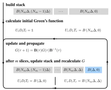
B(Nm ,(Nm 1) )

B(Nm ,0)

· · ·

build stack

calculate initial Green’s function

update and propagate

G(⌧+ 1) =B(⌧)G(⌧)B ¹(⌧)

after m slices, update stack and recalculate G

· · · B(Nm , ) B( ,0)

UlDlTl=B( ,0) UrDrTr=B(Nm , ) UrDrTr=B(Nm ,0)

Figure 2.2.: Flow diagram of the DQMC algorithm. Shaded in grey is the initial build-up of the stack of decomposed matrix products. This is used to calculate the Green’s function which is subsequently updated and propagated in imaginary time before updating the stack and recalculating the Green’s function from the stack to ensure stability. The slice product B(∆,1) shaded in blue has to be recalculated from scratch because it contains auxiliary field values that were updated in the Monte Carlo procedure. Subsequent slice products will the respective preceding U matrix as a starting point for the recalculation. Figure first appeared in [25].

Making use of the stack

For those imaginary time slices where the Green’s function has to be recalculated from scratch, one can greatly facilitate its calculation by making use of the matrix products saved in the stack. After building up the stack in an initial procedure, the last entry con- tains the decomposed product over all slice matrices, the previous entry has all matrices but the last m slices and so forth. Updates starting at the last slice, i.e. down from the

"top" of the stack. After m updates have been performed, the Green’s function has to be recalculated at the same time slice. The stack already contains the decomposed product of all matrices from τ = 1 up until the current time slice, called U _L D _L T _L . Thus, only the decomposed product for the sequence starting at the current time slice up until τ = β , de- noted by U _R D _R T _R , is needed. The entire slice product is then given as U _L D _L T _L U _R D _R T _R , but it is not necessary to actually carry out the recombination. The product of left and right decomposition can be directly used in equations (2.39) and (2.40) by making slight changes to (2.41).

A summary and overview of the DQMC algorithm are presented in Fig. 2.2.

3. Stochastic Series Expansion

Stochastic Series expansion (SSE) [26, 27] is a highly efficient Monte Carlo flavor mainly used for the simulation of bosonic quantum mechanical systems. It can be formulated in both a finite temperature and a ground state setting, which work almost identically.

This chapter aims to convey the basics of the finite temperature formulation which was employed to collect some of the data presented in the later chapters. Similarly structured as the preceding chapter 2, this chapter first introduces the basic idea of the SSE algorithm and then proceeds to describe update and measurement schemes.

3.1. Formulation of the Monte Carlo procedure

The key idea of SSE is to rewrite the partition sum in its power series representation Z = Tr exp ( − β H) = ∑

| ψ i

h ψ |

∑ ∞ n=0

β ⁿ

n! ( − H) ⁿ | ψ i . (3.1) This approach is based on Handscomb’s method [28] but it had to reformulated to be successfully applied to a variety of models [29, 30, 31, 32, 33]. For each power in the expanded series, a resolution of unity | φ _i ih φ _i | is inserted to give

Z = ∑

| ψ i

∑ ∞ n=0

β ⁿ

n! h ψ | ( − H) | φ ₁ ih φ ₁ | ( − H) | φ ₂ ih φ ₂ | . . . | φ _{n − 1} ih φ _{n − 1} | ( − H ) | ψ i . (3.2) Evaluating all of the expectation values for all combinations is impossible which moti- vates the use of Monte Carlo to sample the terms that contribute most to the partition sum. Each Hamiltonian operator is then broken up into smaller units, most often into bond operators. In some cases, larger clusters are possible and sometimes advantageous or even necessary to use [34, 35]. In any case, the Hamiltonian is then written as

H = − ∑

t ∑

l

H _t,u . (3.3)

Each term is indexed by its operator type t, e.g. a diagonal S _z interaction or an off- diagonal spin exchange, and by the index of the lattice unit u, e.g. the number of the bond this operator acts on. To shorten the long multiplication that results when (3.3) is inserted into (3.2), the many different combinations of operators are encoded in a new object called operator sequence, denoted by S _n . This allows writing the partition function in the following concise way:

Z = ∑

| ψ i

∑ ∞ n=0 ∑

S

β ⁿ n!

∏ n

i=1 h φ _{i − 1} | H _t

_,u

| φ _i i . (3.4)

In this expression, the identification | ψ i ≡ | φ ₀ i ≡ | φ _n i has been made in favor of a clearer notation. Although there is a sum over all expansion orders n ∈ [0, ∞], it turns out that in practice there is an effective maximum expansion order M that suffices to capture all relevant sequence lengths. Its precise value is determined dynamically in the course of the simulation. In contrast to DQMC and other worldline techniques, there is, therefore, no additional approximation error other than the statistical error from the Monte Carlo sampling. Any sequence of shorter length n < M can be artificially enlarged to one of size M by considering all possible arrangements of n operators on M places and filling the remaining slots with identity operators. When writing the operator sequence in such a way, the contribution of any shorter sequences their contribution to the final expression has to be corrected by a factor (M − n)! / M! to avoid overcounting:

Z = ∑

| ψ i ∑

S

(M − n)!

M!

β ⁿ n!

∏ M

i=1 h φ _{i − 1} | H _t

_,u

| φ _i i (3.5) Note that β still comes with a power n because it depends on how many non-trivial ele- ments are contained in the extended operator sequence.

3.2. Sampling operator sequences

Moving along the Markov chain and proposing new operator sequences follows a set of well defined, general rules which are nevertheless easiest to illustrate on a concrete example. For this purpose, the anisotropic Heisenberg model in a magnetic field is used which will reappear in chapter 6. Its Hamiltonian is

H = − ∑

h i, j i

S ⁺ _i S ⁻ _j + S ⁻ _i S ⁺ _j

+ ∆ ∑

h i, j i

S ^z _i S ^z _j + h ∑

i

S ^z _i , (3.6)

and the simulation is carried out in the S ^z basis. The first term is a sum of off-diagonal operators responsible for exchanging spins of opposite orientation. The second term is diagonal in the simulation basis and simply measures the relative orientation of two spins, while the third one compares the orientation of each individual spin to the direction of the magnetic field. Following the rules for the formulation of the partition sum laid out previously, each of the sums in the Hamiltonian is rewritten in terms of bond operators. In fact, the first and the second term are already of the correct form, but the coupling to the magnetic field requires a little work. To make it compatible with the bond formulation, its contribution is distributed over the adjacent bonds of each site giving rise to a magnetic field h _B = h/4. Ultimately, there are thus only two possible types of operators, which are the diagonal operator

H _diag = ∆S ^z _i S ^z _j + h _B (S ^z _i + S ^z _j ) , (3.7) and the off-diagonal operator

H _exchange = −

S ⁺ _i S ⁻ _j + S _i ⁻ S ⁺ _j

. (3.8)