Threshold Selection, Hypothesis Tests, and DOE Methods

Threshold Selection, Hypothesis Tests, and DOE Methods

Thomas Beielstein

Department of Computer Science XI, University of Dortmund, D-44221 Dortmund, Germany.

tom@ls11.cs.uni-dortmund.de Sandor Markon

FUJITEC Cm.Ltd. World Headquarters, 28-10, Shoh 1-chome, Ibaraki, Osaka, Japan.

markon@rd.fujitec.co.jp

Abstract- Threshold selection – a selection mechanism for noisy evolutionary algorithms – is put into the broader context of hypothesis testing. Theoretical results are pre- sented and applied to a simple model of stochastic search and to a simplified elevator simulator. Design of experi- ments methods are used to validate the significance of the results.

1 Introduction

Many real world optimization problems have to deal with noise. Noise arises from different sources, such as measure- ments errors in experiments, the stochastic nature of the sim- ulation process, or the limited amount of samples gathered from a large search space. Evolutionary algorithms (EA) can cope with a wide spectrum of optimization problems [16].

Common means used by evolutionary algorithms to cope with noise are resampling, and adaptation of the population size.

Newer approaches use efficient averaging techniques, based on statistical tests, or local regression methods for fitness es- timation [3, 1, 17, 6, 15].

In the present paper we concentrate our investigations on the selection process. From our point of view the following case is fundamental for the selection procedure in noisy envi- ronments: Reject or accept a new candidate, while the avail- able information is uncertain. Thus, two errors may occur:

An

error as the probability of accepting a worse candidate due to noise and a

error, the error probability of rejecting a better candidate.

A well established technique to investigate these error prob- abilities is hypothesis testing. We state that threshold selec- tion (TS) can be seen as a special case of hypothesis testing.

TS is a fundamental technique, that is used also used in other contexts and not only in the framework of evolutionary algo- rithms. The TS-algorithm reads: Determine the (noisy) fitness values of the parent and the offspring. Accept the offspring if its noisy fitness exceeds that of the parent by at least a margin of

; otherwise retain the parent.

The theoretical analysis in [13], where TS was introduced for EAs with noisy fitness function values, were based on the progress rate theory on the sphere model and were shown for the

⁽¹⁺¹⁾

-evolution strategy (ES). These results were subse-

quently transfered to the S-ring, a simplified elevator model.

Positive effects of TS could be observed. In the current paper we will base our analysis on mathematical statistics.

This paper is organized as follows: In the next section we give an introduction into the problems that arise when selec- tion in uncertain (e.g. noisy) environments takes place. The basic idea of TS is presented in the following section. To show the interconnections between the threshold value and the critical value, statistical hypothesis testing is discussed.

Before we give a summary, we show the applicability of TS to optimization problems: A stochastic search model – simi- lar to the model that was used by Goldberg in his investiga- tion of the mathematical foundations of Genetic Algorithms – and the S-ring – a simplified elevator simulator – are inves- tigated [7, 13].

2 Selection in Uncertain Environments

Without loss of generality we will restrict our analysis in the first part of this paper to maximization problems. A candidate is ‘better’ (‘worse’), if its fitness function value is ‘higher’

(‘lower’) than the fitness function value of its competitor. Sup- pose that the determination of the fitness value is stochasti- cally perturbed by zero mean Gaussian noise. Let

^f~

denote the perturbed fitness function value, while

^f

denotes the av- erage fitness function value. Obviously four situations may arise in the selection process: A

^f

better

^j

worse

^g

candidate can be

^f

accepted

^j

rejected

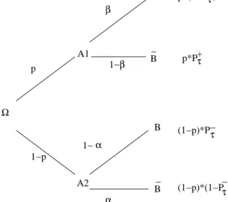
^g

. This situation is shown in Fig. 1. The chance of accepting a good (respectively of re- jecting a worse) candidate plays a central role in our investi- gations. In the next section, we shall discuss the details of the TS process.

3 Threshold Selection

3.1 Definitions

Threshold selection is a selection method, that can reduce the

error probability of selecting a worse or rejecting a good can-

didate. Its general idea is relatively simple and already known

in other contexts. Nagylaki states that a similar principle is

very important in plant and animal breeding: Accept a new

candidate if its (noisy) fitness value is significantly better than

1

β

α Ω

A1 p

1−p

α

B B

_ 1−β

B

B A2 _

p*P + p*(1−P +

)

(1−p)*P−

(1−p)*(1−P ) − τ τ

τ τ

1−

Figure 1: Decision tree visualizing the general situation of a se- lection process in uncertain environments. The events are labeled as follows:

^A1

:

^{f(Y) >f(X)}

,

^A2

:

^{f(Y) f(X)}

,

^B

:

^{f(Y) <}

f(X)

, and

^B

:

^f(Y)f(X)

. that of the parent [14].

D EFINITION 1 (T HRESHOLD A CCEPTANCE P ROBABILITY ) Let

^{f(X) :=}

P

n

i=1

~

f(X

i

)=n

be the sample average of the perturbed values, and

^f

denote the unperturbed fitness func- tion value. The conditional probability, that the fitness value of a better candidate

^Y

is higher than the fitness value of the parent

^X

by at least a threshold

,

P +

:=Pff(Y)>f(X)+ jf(Y)>f(X)g;

(1) is called a threshold acceptance probability.

D EFINITION 2 (T HRESHOLD R EJECTION P ROBABILITY ) The conditional probability, that a worse candidate

^Y

has a lower noisy fitness value than the fitness value of parent

^X

by at least a threshold

,

P

:=Pff(Y)f(X)+ jf(Y)f(X)g:

(2) is called a threshold rejection probability.

The investigation of the requirements for the determina- tion of an optimal threshold value reveals similarities between TS and hypothesis tests.

4 Hypothesis Tests

4.1 Hypothesis and Test Statistics

The determination of a threshold value can be interpreted in the context of hypothesis testing as the determination of a critical value. To formulate a statistical test, the question of interest is simplified into two competing hypotheses between

which we have a choice: the null hypothesis, denoted

^H0

, is tested against the alternative hypothesis, denoted

^H1

. The

-2 2 4 d

0.1 0.2 0.3 0.4 f

-2 2 4 d

0.1 0.2 0.3 0.4 f

Figure 2: Error of the first (light region) and of the second kind (darkest region): P.d.f. of two normal-distributed r.v.

^XN(0;1)

and

^{Y N(2;1)}

.

decision is based on a quantity

^T

calculated from a sample of data using a test function or test statistic. In the following we will use the r. v.

Z

m;n :=

1

n n

X

i=1

~

f(Y

t;i )

1

m m

X

i=1

~

f(X

t;i

)

(3) as a test function.

^m

and

ⁿ

define the number of samples taken from the parent

^Xt

respectively offspring

^Yt

at time step

t

.

4.2 Critical Value and Error Probabilities

The critical value

^c1

for a hypothesis test is a threshold to which the value of the test statistic in a sample is compared to determine whether or not the null hypothesis is rejected. We are seeking a value

^c1

, such that

PfT>c

1 jH

0

true

^g:

(4) Making a decision under this circumstances may lead to two errors: an error of the first kind occurs when the null hypoth- esis is rejected when it is in fact true; that is,

^H0

is wrongly rejected with an error probability

. If the null hypothesis

^H0

is not rejected when it is in fact false, an error of the second kind happens.

denotes the corresponding error probability.

5 Hypothesis Testing and Threshold Selection

5.1 The Relationship between

,

, and

^P

Let us consider the hypothesis

^H0

, that the fitness of the off- spring is not better than the parental fitness. Furthermore we will use the test function defined in Eq. 3. Regarding selection in uncertain environments from the point of view of hypothe- sis tests, we obtain:

T HEOREM 5.1

Suppose that

^{T = Z}m;n

,

^c1

=

, and

^H0 : f(Y

t )

f(X

t

)

. Then we get: The conditional rejection probability

2

P

and the error of the first kind are ‘complementary’ prob- abilities.

P

=PfZ

m;n

>jf(Y

t

)f(X

t

)g=1 :

(5) Proof This can be seen directly by combining Eq. 2 and Eq.4.

C OROLLARY 5.2 ( TO THEOREM 5.1) The conditional acceptance probability

^P+

and the error of the second kind are ‘complementary’ probabilities:

P +

=1 :

(6)

5.2 Normal Distributed Noise

In the following,

^(x)

denotes the normal d.f., whereas

^z

defines the

⁽⁾

-quantile of the

^N(0;1)

-distribution:

^(z )=

, and

^t

defines the

⁽⁾

-quantile of the

^t

-distribution. We are able to analyze TS with the means of hypothesis tests:

Assuming stochastically independent samples

^Xt;i

and

^Yt;i

of

^N(X

; 2

X

)

respectively

^N(Y

; 2

Y

)

distributed variables, we can determine the corresponding threshold

for given er- ror of the first kind

. The equation

^PfZm;n

jH

0 g =

1

leads to

=z

1

r

2

X

m +

2

Y

n

:

(7)

5.3 Unknown, but Equal Variances

²

X

and

²

Y

In many real world optimization problems, the variances are unknown, so that the test is based on empirical variances:

Let the r.v.

S 2

X :=

1

m 1 m

X

i=1 (

~

f(X

t;i

) f(X

t ))

2

(8)

be the empirical variance of the sample. In this case, we ob- tain:

= ( t

m+n 2;1 )

s

(m 1)s 2

x

+(n 1)s 2

y

n+m 2

r

m+n

mn :

(9)

If the observations are paired (two corresponding programs are run with equal sample sizes (

^{m= n}

) and with the same random numbers) and the variance is unknown, Eq. 9 reads:

= t

n 1;1 s

d

p

n

;

(10)

with

s 2

d

= 1

n 1 n

X

i=1 (z

i d)

2

;

(11)

an estimate of the variance

²

d

, and

d= P

m

i=1 n

~

f(Y

t;i )

~

f(X

t;i )

o

=m

.

These results provide the basis for a detailed investigation of the TS mechanism. They can additionally be transferred to real-world optimization problems as shown in the following sections.

6 Applications

6.1 Example 1: A Simple Model of Stochastic Search in Uncertain Environments

In our first example, we analyze the influence of TS on the selection process in a simple stochastic search model. This model possesses many crucial features of real-world optimiza- tion problems, i. e. a small probability of generating a better offspring in an uncertain environment.

6.1.1 Model and Algorithm

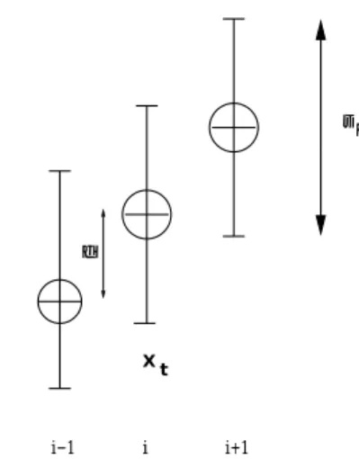
D EFINITION 3 (S IMPLE S TOCHASTIC S EARCH )

Suppose that the system to be optimized is at time

^t

in one of the consecutive discrete states

^Xt

=i

,

^{i 2ZZ}

. In state

ⁱ

, we can probe the system to obtain a fitness value

^f~(Xt

) =

i+U

.

^{2 IR+}

represents the distance between the ex- pectation of the fitness values of two adjacent states. The random variable (r.v.)

^U

possesses normal

^N(0;2

)

distri- bution. The goal is to take the system to a final state

^Xt

=i

with

ⁱ

as high as possible (maximization problem) in a given number of steps.

i i+1

i−1 δ

σ ε

Xt

Figure 3: Simple stochastic search. Adjacent states.

Let us consider the following

A LGORITHM 1 (S IMPLE S EARCH WITH TS) 1. Initialize: Initial state

^Xt=0

=0

.

2. Generate offspring: At the

^t

-th step, with current state

X

t

= i

, flip a biased coin: Set the candidate of the new state

^Yt

to

ⁱ⁺¹

with probability

^p

and to

^{i 1}

with probability

^{(1 p)}

.

3. Evaluate: Draw samples (fitness values) from the current and the candidate states:

~

f(X

t;j

)

and

^f~(Yt;k

);

(12)

with the measured fitness value

^{f~(X) := f(X)+w}

.

w

is the realization of a r.v., representing normal dis- tributed noise,

^{W N(0;2}

)

.

3

4. Select: Determine a threshold value

. If

^f(Yt

)+ >

f(X

t

)

, accept

^Yt

as the next state:

^Xt+1 :=Y

t

; other- wise , keep the current state:

^Xt+1

:=X

t

. 5. Terminate: If

^t<tmax

, increment

^t

and go to step 2.

R EMARK 1

In this model,

^p

is given; it is interpreted as the probability of generating a better candidate. In general, the experimenter has no control over

^p

, which would be some small value for non-trivial optimization tasks.

T HEOREM 6.1

A LGORITHM 1 can be represented by a Markov chain

^fXt g

with the following properties:

1.

^X0

=0

. 2.

^PfXt+1

=i+1jX

t

=ig=pP +

3.

^PfXt+1

=i 1jX

t

=ig=(1 p)(1 P

)

4.

^PfXt+1

=ijX

t

=ig=p(1 P +

)+(1 p)P

, with

P

:=

0

@

q

m+n

mn

1

A

:

(13)

6.1.2 Search Rate and Optimal

The measurement of the local behavior of an EA can be based on the expected distance change in the object parameter space.

This leads to the following definition:

D EFINITION 4 (S EARCH R ATE )

Let

^R

be the number of advance in the state number

^t

in one step:

R:=X

t+1 X

t

:

(14)

The search rate is defined as the expectation

E[R(;

;p;t)];

(15) to be abbreviated

^E[R]

.

T HEOREM 6.2 Let

^E[R

]

be the search rate as defined in Eq. 15. Then Eq. 13 leads to

E[R

]=pP +

(1 p)(1 P

):

(16) C OROLLARY 6.3 ( TO THEOREM 6.2)

In this example (simple stochastic search model) it is pos- sible to determine the optimal

opt

value with regard to the search rate, if the fitness function is disturbed with normal- distributed noise:

opt

=

2

log

1 p

p

:

(17)

p

opt

E[R

=0

] E[R

opt ]

0.1 4.394 -0.262 0.00005

0.2 2.773 -0.162 0.003

0.3 1.695 -0.062 (D) 0.018 (C)

0.4 0.811 0.038 (B) 0.059 (A)

0.5 0.0 0.138 0.138

Table 1: Simple stochastic search. The noise level

equals

^1:0

, the distance

is

^0:5

. Labels (A) to (D) refer to the results of the corresponding simulations shown in Fig. 4.

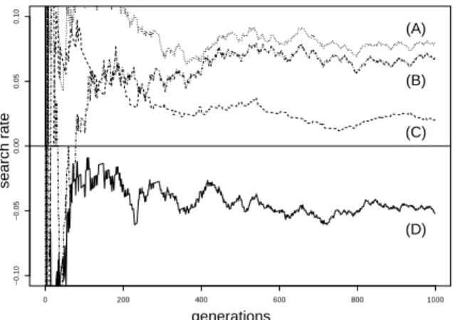
0 200 400 600 800 1000

−0.10−0.050.000.050.10

(A)

(B)

(C)

(D)

generations

search rate

Figure 4: Simple stochastic search. Simulations performed to ana- lyze the influence of TS on the search rate.

Assume there is a very small success probability

^p

. Then the search can be misled, although the algorithm selects only

‘better’ candidates. We can conclude from Eq. 16, that a decreasing success probability (

^{p & 0}

) leads to a negative search rate. Based on Eq. 17, we calculated the optimal thresh- old value for 5 different success probabilities to illustrate the influence of TS on the search rate, cp. Tab 1. Corresponding values of the search rate are shown in the third column. TS can enhance the search rate and even avoid that the search rate becomes negative. This can be seen from the values in the last column.

Fig. 4 reveals that simulations lead to the same results. For two different

^p

-values, the influence of TS on the search rate is shown. The search rate becomes negative, if

^p

is set to

0:3

and no TS is used (D). The situation can be improved, if we introduce TS: The search rate becomes positive (C). A comparison of (A), where a zero threshold was used, and (B), where the optimal threshold value was used, shows that TS can improve an already positive search rate. These results are in correspondence with the theoretical results in Tab. 1.

6.2 Example 2: Application to the S-ring Model 6.2.1 The S-Ring as a Simplified Elevator Model

In the following we will analyze a ‘S-ring model’, that is a

simplified version of the elevator group control problem [12,

4

13]. The S-ring has only a few parameters: the number of el- evator cars

^sm

, the number of customers

^sn

, and the passen- ger arrival rate

^s

. Therefore, the rules of operation are very simple, so that this model is easily reproducible and suitable for benchmark testing. However, there are important similar- ities with real elevator systems. The S-ring and real elevator systems are discrete-state stochastic dynamical systems, with high-dimensional state space and a very complex behavior.

Both are found to show suboptimal performance when driven with simple ‘greedy’ policies. They exhibit a characteristic instability (commonly called ‘bunching’ in case of elevators).

The policy

, that maps system states to decisions, was rep- resented by a linear discriminator (perceptron) [13]. An EA was used to optimize the policy

.

6.2.2 DOE-Methodology

The analysis of many real-world optimization problems re- quires a different methodology than the analysis of the opti- mization of a fitness function

^f

, because

^f

remains unknown or can only be determined approximately. We use an ap- proach that is similar to the concept discussed in [8]: From the complex real-world situation we proceed to a simulation model. In a second step we model the relationship between the inputs and outputs of this model through a regression model (meta-model). The analysis of the meta-model is based on DOE methods. Let the term factor denote a parameter

Factor low value medium

value

high value (A)Selection: comma-

strategy

plus- strategy

TS-strategy (B)Selective Pres-

sure:

4.0 6.0 9.0

(C)Population Size:

2.0

⁴

7.0

Table 2: EA–parameter and factorial designs

−3 −2 −1 0 1 2 3

2.352.45

Normal Q−Q Plot

Theoretical Quantiles

Sample Quantiles

Figure 5: Diagnostic plot.

or input variable of our model. DOE methods can be de- fined as selecting the combinations of factor levels that will be actually simulated when experimenting with the simulation

model [5, 4, 8, 9, 11, 10]. It seems reasonable to use DOE methods on account of the exponential growth in the num- ber of factor levels as the number of factors grows. Based on these methods, we investigate the S-ring model

¹

. The princi- pal aim is to minimize the number of waiting customers, so we consider a minimization problem. A prototype S-ring

2.352.402.45

total

2.352.402.45

Comma

2.352.402.45

Plus

2.352.402.45

TS

Figure 6: Box plot. Different selection schemes. Comma-selection, plus-selection, and TS, cp. Tab. 2.

2.3902.3952.4002.405

0 1 2

B

4 6 9

Comma Plus TS

2.382.392.402.412.42

0 1 2

C

2 4 7

Comma Plus TS

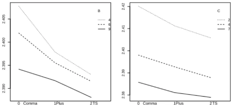
Figure 7: Plot of the means of the responses. The labels on the

x

-axis represent different selection mechanism.

⁰

: Comma,

¹

: Plus, and

²

: TS.

^B

and

^C

represent the selective strength

^(4;6;9)

, resp.

the population size

^(2;4;7)

, cp. Tab. 2.

with the following parameter settings was used as a test case:

customers

^sn

=6

, servers

^sm

=2

, and arrival rate

^s

=0:3

. The number of fitness function evaluations was set to

¹⁰⁵

, and every candidate was reevaluated 5 times. Eq. 10 was used to determine the threshold. The TS-scheme was compared to a comma-strategy and a plus-strategy. Global intermediate recombination was used in every simulation run.

⁵⁰

exper- iments were performed for every ES-parameter setting. The population size and the selective pressure (defined as the ratio

=

) were varied. The corresponding settings are shown in Tab. 2.

6.2.3 Validation and Results

Before we are able to present the results of our simulations, the underlying simulation model has to be validated. The nor-

1

The applicability of DOE methods to EAs is discussed in detail in [2].

5

mal Q–Q plot in Fig. 5 shows that the values are approxi- mately standard normal. This is an important assumption for the applicability of the F-test, that was used in the regression analysis to determine the significance of the effects and of the interactions. Further statistical analysis reveals that the effects of the main factors are highly significant.

The results are visualized in two different ways. Box plots, shown in Fig. 6, give an excellent impression how the change of a factor influences the results. Comparing the comma- selection plot and the plus-selection plot to the TS selection plot, we can conclude that TS improves the result. In addition to the box plots, it may be also important to check for inter- action effects (Fig. 7): Obviously TS performs better than the other selection methods.

7 Summary and Outlook

The connection between TS and hypothesis tests was shown.

A formulae for the determination of the optimal

value in a simple search model and a formulae for the determination of the threshold value for the error of the first kind

and the (es- timated) variance

^s2

d

were derived. Theoretical results were applied to a simplified elevator group control task problem.

TS performs significantly better than other selection methods.

This work will be extended in the following way: To re- duce the number of fitness function evaluations it might be sufficient to determine the noise level only at the beginning and after a certain number of time steps, instead of in ev- ery generation. Furthermore, we will investigate the situation shown in Fig. 1 from the viewpoint of Bayesian statistics.

Acknowledgments

T. Beielstein’s research was supported by the DFG as a part of the collaborative research center ‘Computational Intelli- gence’ (531).

Bibliography

[1] D. V. Arnold. Evolution strategies in noisy environ- ments — A survey of existing work. In L. Kallel, B. Naudts, and A. Rogers, editors, Theoretical Aspects of Evolutionary Computing , Natural Computing, pages 239–249. Springer, Berlin, 2001.

[2] T. Beielstein. Design of experiments and evolution- ary algorithms. Part I: The classical model. Technical report, Universit¨at Dortmund, Fachbereich Informatik, 2001. (to appear).

[3] H.-G. Beyer. Evolutionary algorithms in noisy environ- ments: Theoretical issues and guidelines for practice.

CMAME (Computer methods in applied mechanics and engineering), 186:239–267, 2000.

[4] G. E. P. Box and N. R. Draper. Experimental Model Building and Response Surfaces. Wiley, 1987.

[5] G. E. P. Box, G. Hunter, William, and J. S. Hunter.

Statistics for experimenters. Wiley series in probabilty and mathematical statistics: Applied probability and statistics. Wiley, 1978.

[6] J. Branke, C. Schmidt, and H. Schmeck. Efficient fit- ness estimation in noisy environments. In L. S. et al., editor, Genetic and Evolutionary Computation Confer- ence (GECCO’01). Morgan Kaufmann, 2001.

[7] D. E. Goldberg. Genetic Algorithms in Search, Op- timization, and Machine Learning . Addison-Wesley, 1989.

[8] J. Kleijnen. Statistical Tools for Simulation Practition- ers. Marcel Dekker, New York, 1987.

[9] J. Kleijnen. Validation of models: Statistical techniques and data availability. In P. Farrington, H. Nembhard, D. Sturrock, and G. Evans, editors, Proceedings of the 1999 Winter Simulation Conference , pages 647–654, 1999.

[10] J. Kleijnen. Experimental designs for sensitivity analy- sis of simulation models. In A. H. et al, editor, Proceed- ings of EUROSIM 2001, 2001.

[11] A. M. Law and W. D. Kelton. Simulation Modelling and Analysis. McGraw-Hill Series in Industrial Egineering and Management Science. McGraw-Hill, New York, 3 edition, 2000.

[12] S. Markon. Studies on Applications of Neural Networks in the Elevator System. PhD thesis, Kyoto University, 1995.

[13] S. Markon, D. V. Arnold, T. B¨ack, T. Beielstein, and H.-G. Beyer. Thresholding – a selection operator for noisy es. In J.-H. Kim, B.-T. Zhang, G. Fogel, and I. Kuscu, editors, Proc. 2001 Congress on Evolutionary Computation (CEC’01), pages 465–472, Seoul, Korea, May 27–30, 2001. IEEE Press, Piscataway NJ.

[14] T. Nagylaki. Introduction to Theoretical Population Ge- netics. Springer, Berlin, Heidelberg, 1992.

[15] Y. Sano and H. Kita. Optimization of Noisy Fitness Functions by Means of Genetic Algorithms using His- tory of Search. In M. Schoenauer, K. Deb, G. Rudolph, X. Yao, E. Lutton, J. Merelo, and H.-P. Schwefel, edi- tors, Parallel Problem Solving from Nature (PPSN VI), volume 1917 of LNCS, pages 571–580. Springer, 2000.

[16] H.-P. Schwefel. Evolution and Optimum Seeking . Sixth- Generation Computer Technology. Wiley Interscience, New York, 1995.

[17] P. Stagge. Averaging efficiently in the presence of noise.

In A.Eiben, editor, Parallel Problem Solving from Na- ture, PPSN V, pages 188–197, Berlin, 1998. Springer- Verlag.

6