Mathematical Ecology
Joachim Hermisson, Claus Rueffler & Meike Wittmann
∗April 16, 2020
Literature and Software
• Sarah P. Otto, Troy Day: A Biologist’s Guide to Mathematical Modeling in Ecology and Evolution, Princeton University Press (∼72 Euro)
• Mark Kot: Elements of Mathematical Ecology, Cambridge University Press (∼ 62 Euro)
• Josef Hofbauer and Karl Sigmund: Evolutionary Games and Population Dynamics, Cambridge University Press (∼49 Euro)
• Linda Allen: An Introduction to Stochastic Processes with Applications to Biology, Prentice Hall (∼70 Euro)
• Peter Yodzis: Introduction to Theoretical Ecology (1989), Harper & Row.
This book is out of print. A pdf can be downloaded from
www.rug.nl/research/institute-evolutionary-life-sciences/tres/ downloads/bookyodzis.pdf
• Gerald Teschl: Ordinary Differential Equations and Dynamical Systems, American Mathematical Society, pdf online at www.mat.univie.ac.at/ gerald/ftp/book-ode/
• Populus simulation and visualization software: http://cbs.umn.edu/populus/overview
Ecology
Oikos = house, dwelling place. Logos = word, study of. Ecology refers to the scientific study of living organisms in their natural environment. It is a diverse scientific discipline and covers various levels of biological organization.
• On the individual level, physiological ecology discusses the influence of food, light, humidity, pesticide concentrations, etc, on the life histories of individuals.
∗First version 2012 by JH and CR, revised and extended JH and MW 2015, edits JH 2018, 2020.
• Population ecology studies the interactions of populations with their environment, with consequences on population structure and demography. On the same level, behavioral ecology discusses the consequences of different behavioral strategies.
• Finally, community ecology and ecosystems ecologytreat the fate of complex ecosys- tems with anything from two to tens of thousands of interacting species and groups of species.
Ecology is closely related to evolution and the interactions of population dynamics and evolution are the subject of evolutionary ecology. Many branches of ecological research use mathematical models. For example, behavioral ecology makes use of game theoretical methods to explore the impact of behavioral strategies. Evolutionary ecology draws heavily on the mathematical models of evolutionary genetics. The focus of this lecture must be much more narrow. It will mainly be on population ecology, where we study the dynamics of population sizes, equilibria, growth and extinction, under various ecological boundary conditions. We will make a few side-steps into evolutionary ecology, but we won’t treat aspects of behavior and we won’t cover inheritance and the dynamics of genotypes. These topics are devoted to the specialized lectures on game theory and on population genetics.
Ecological Modeling
Any biological model is a map of some part of Nature to a mathematical formalism. Models are always abstractions, i.e. simplifying representations of reality. Modeling thus starts with a series of model assumptions: some aspects of Nature are integrated into the model, because we assume that they are essential for the problem at hand. Many other aspects are ignored (or abstracted from), either because they are much less important or because we want to take a reductionist perspective. In the latter case, we hope that we can understand a complex system by studying of several (sets of) factors one by one. As an example, if we want to model future population size in Austria, the current size and age structure are certainly essential. Other factors like progress in medical treatment might also have some impact on death rates, but can be ignored in a simple model. Still other factors, such as immigration, are likely important, but a treatment without immigration may already provide us with some valuable information and we may want to study the impact of immigration in a separate step.
With an increasing number of factors included, a model gets more precise and spe- cific. This is needed, in particular, for reliable quantitative predictions (weather forecast, demographic models). However, added complexity always means reduced manageability and often also reduced generality. From a model that is as complex as the system that it represents we cannot obtain any new insights. Complex quantitative models that are used for predictions can usually only be treated by computer simulations. In contrast, many questions we might ask are of qualitative nature (e.g., whether population size approaches an equilibrium or whether there will be cycles). In these cases, one often aims for a minimal set of factors to explain a phenomenon.
The art of modeling thus consists of selecting the essential factors to include in a model.
On the one hand, this requires experience and some knowledge of the biological system of interest. On the other hand, this also requires an understanding of the mathematical mechanism, in order to see which factors can have crucial consequences, even if they may look like small effects initially. As such, ecological modeling relies on a broad mathematical tool-box, including elements from the theory of stochastic processes, dynamical systems, differential equations, and statistics.
1 Dynamics of single, unstructured populations
The dynamical process of population growth and decline is a function of factors that are intrinsic to a population (e.g., its potential to reproduce, its life-cycle, or its density) and the environmental conditions. The environment comprises all resources that are essential for a population to thrive, like food and space, and factors that may reduce its size, such as predation and disease. In nature, many of these factors are indeed reproducing popu- lations themselves, which can act as predators, competitors, or as food resource. As such, these populations should follow their own population dynamics. Since the dynamical pro- cesses of (e.g.) predators and prey interact, we quickly obtain a complex multi-dimensional problem. We deal with these complexities further on. As our first step, we make the sim- plifying assumption that we can ignore all interactions with other dynamical aspects of the environment and just model the dynamics of a single population. This can sometimes be justified if the dynamics of all interacting populations happens on different time scales:
either much faster, such that we can always assume that the interacting population is at a dynamical equilibrium, or much slower, such that the size of an interacting population does not change much over time-spans of interest. We also assume that the population is unstructured. This means, all individuals of the population are treated as equal. In par- ticular, there are no age classes, no phenotypic differences (of relevance to the dynamics), and we can ignore the distribution of the population across physical space.
1.1 Birth and death processes
We describe the development of a population through time as a dynamical process. For a single, unstructured population, we have a single dynamic variable N(t), measuring the population size or population density (individuals per square meter) at timet. The variable N(t) may be affected by various demographic events, such as:
• birth
• death
• immigration and emigration
Demographic events in nature are stochastic. In the most explicit “individual based” de- mographic models, the population dynamics is therefore described as a stochastic process.
Define PN(t) as the probability to observe N individuals at time t. We assume that each individual can give birth at a constant rateb and may die at rate d. Birth and death occurs for all individuals independently of all other individuals and independently of age.
Formally, the process then follows a continuous-time Markov chain with statesN ∈Nand time-homogeneous transition probabilities. We have:
PN(t+ ∆t) = (N −1)b∆tPN−1(t) + (N + 1)d∆tPN+1(t) + (1−N b∆t−N d∆t)PN(t) (1) and thus in the limit ∆t→0 (Kolmogorov forward equation orMaster equation):
P˙N(t) = ∂PN(t)
∂t =d(N + 1)PN+1(t) +b(N −1)PN−1(t)−N(b+d)PN(t) (2) with some initial condition PN(0) = 1 for N = N0 and PN(0) = 0 else. (In particular, we have PN(t) = 0 for all N < 0 and all t.) The Master equations are a system of infinitely many ordinary differential equations. We consider the expected population size
N¯(t) =
∞
X
N=0
N PN(t). (3)
From the Master equation follows
∂N¯
∂t =
∞
X
N=0
N∂PN(t)
∂t
=
∞
X
N=0
dN(N + 1)PN+1(t) +bN(N −1)PN−1(t)−N2(b+d)PN(t)
=
∞
X
N=0
d(N −1)N PN(t) +b(N + 1)N PN(t)−N2(b+d)PN(t)
=
∞
X
N=0
N(b−d)PN(t)
= (b−d) ¯N(t) (4)
Defining the net growth rate r=b−d, we obtain the solution
N¯(t) = N0·exp[rt]. (5)
We thus see that the expected value of the stochastic process follows simple exponential growth. The long-term behavior follows a simple dichotomy: the expected population size declines to zero as the population dies out for d > b, while it grows without bounds for b > d. However, the behavior of the stochastic process is richer than predicted just by the expected value. Similar to the derivation above, we can derive the variance. We start with
the dynamics of the second moment:
∂N2
∂t =
∞
X
N=0
N2∂PN(t)
∂t
=
∞
X
N=0
dN2(N+ 1)PN+1(t) +bN2(N −1)PN−1(t)−N3(b+d)PN(t)
=
∞
X
N=0
d(N−1)2N PN(t) +b(N + 1)2N PN(t)−N3(b+d)PN(t)
=
∞
X
N=0
(2N2(b−d) +N(b+d))PN(t)
= 2(b−d)N2(t) + (b+d) ¯N(t). (6) Defining N2(t) := Q(t)N0exp(rt) and with the solution for ¯N(t) from above, we obtain:
Q(t) = (b˙ −d)Q(t) + (b+d) (7)
which is solved by
Q(t) = Cexp(rt)−b+d b−d.
With Var[N(t)] = N2(t)−( ¯N(t))2 and the boundary condition Var[N(0)] = 0 we now obtain C=N0+ (b+d)/(b−d) and thus
Var[N(t)] = b+d
b−d exp(rt)−1
exp(rt)N0. (8)
Just like the expected value, the variance increases exponentially with time ifb > d. What kind of biological consequences does this stochastic scattering around the expected value have? Most significantly, since extinction (N = 0) is a stationary point of the process, we may ask for the probability that this point is reached from a starting population N =N0. Define uN as the probability that a population of current size N will go extinct at some time in the future. How can we deriveuN? We know the following:
1. Birth and death is independent for all individuals in our model. The population will go extinct if and only if none of the individuals in the starting population will leave offspring in the distant future. Letu=u1 be the probability that a single individual does not leave any offspring. Because of independence, we have uN =uN.
2. Consider a population currently in state N. We may ask for the state of our popula- tion right after the next demographic event, i.e., after a single birth or death. From our current stateN, we can only reach one of the neighboring states. For given birth and death rates b and d, we will be in state N + 1 with probability b/(b+d) and in state N −1 with probability d/(b+d). We thus obtain the following recursion for our extinction probabilities,
uN = b
b+duN+1+ d
b+duN−1 for N ≥1, (9)
with boundary condition u0 = 1. Formally, this corresponds to the transition matrix of a one-dimensional random walk with absorbing state at 0.
We thus obtain the condition
(b+d)u=bu2+d (10)
The two solutions of this quadratic equation are u(1) = d
b ; u(2) = 1.
For d > b, u = 1 is the only valid solution and we see that extinction is certain. For b > d, the population can escape extinction. However, there is still a probability given by uN0 = uN0 = (d/b)N0 that the population dies out – even if the expected value grows without bounds. Note that this probability becomes uN0 = 1 for r = 0, although the expected population size stays constant in this case. However, for b > d and sufficiently large N0 the extinction probability becomes very small. [A formal proof that u = d/b is the correct solution for d < b requires some further arguments, see lecture on stochastic processes or the book by Kot.]
Stochastic and deterministic models We can interpret a deterministic population model as an approximation to a more detailed stochastic process. For a (linear) birth- death model we have seen that the dynamics of the expected population size reproduces deterministic exponential growth. However, there are important aspects of the stochas- tic dynamics that are not covered by a deterministic model. These differences are most important in small populations, where random fluctuations can easily drive a population to extinction. Once the population size is sufficiently large, the deterministic system is a valid approximation of the stochastic model. This can be justified from the coefficient of variation, which derives as
CV[N(t)] =
pVar[N(t)]
N¯(t) = r 1
N0
b+d
b−d 1−exp(−rt)
. (11)
We see that forr >0 CV[N(t)] is limited for alltand gets small for large initial population size N0. It is straightforward to define more complex stochastic models for population dynamics – even with multiple interacting populations. [Some theory that exists along these lines is summarized in the book by Allen]. However, most of these models cannot be solved and our potential to obtain explicit analytical results is very limited. For this reason, the bulk of population dynamical research uses a deterministic approach. For a general stochastic model of a single, unstructured population with birth, death, and immigration, we obtain
N(t)→N(t) + 1 : b(t, N(t))·N(t) +m(t, N(t)) (12) N(t)→N(t)−1 : d(t, N(t))·N(t) (13)
where b(t, N(t)), d(t, N(t)) and m(t, N(t)) are birth-, death-, and immigration rates, re- spectively, which can depend on the population density and on time. (Note that emigration can be subsumed in the death rates). We then have the expected change
E[∆N|N(t)] =
r(t, N(t))·N(t) +m(t, N(t))
∆t . (14)
This can be transformed into a deterministic process using the following correspondence:
N˙(t) =r(t, N(t))·N(t) +m(t, N(t)). (15) We thus obtain an ODE, which in general can be non-linear and time-dependent. This ODE approximates the dynamics of the stochastic system for large population sizes. (We note that it is generally not true that it represents the - exact - dynamics of the expected population size, like in the linear birth-death model). A general strategy in ecological modeling is to use a deterministic model for derivations and to use stochastic computer simulations as back-up, in order to test the robustness of the results.
1.2 Deterministic models in continuous time
The general deterministic model for the dynamics of a single, unstructured population reads:
N˙(t) =f(N, t) =f(N(t), t) (16) N(t)∈Ris usually interpreted as population density rather than the total size. There are (only) a few models with explicit solutions:
• The most basic model is exponential growth with N˙(t) = rN(t)
and explicit solution N(t) = N0exp(rt). The net growth rate r is also called the Malthusian parameter (Thomas Malthus, 1798: Essay on the Principle of Popula- tion). Exponential growth with r > 0 leads to population explosion and is unsus- tainable in Nature. With r <0, there is a trivial stable equilibrium at N = 0.
• The simplest model with a stable equilibrium population derives from a dynamics with immigration and death (negative growth),
N˙(t) = c−dN(t) with c, d >0 and explicit solution
N(t) = c d+
N0− c d
exp[−dt]. (17)
The model describes the dynamics in a population sink. It also describes pure mi- gration if immigration is constant and emigration occurs with a constant per-capita rate.
• The simplest model with population regulation of a population that can sustain itself is the logistic growth model with
N(t) =˙ rN(t)
1− N(t) K
.
It is characterized by linear density dependence with per-capita growth rate r(1− N/K). The parameter ris also called the intrinsic growth rate. K is the carrying ca- pacity. The explicit solution for the logistic growth model follows (e.g. by separation of variables) as
N(t) = K
1−(1−K/N0) exp[−rt]. (18)
The logistic growth model can even be solved with time-dependent per-capita growth rate r(t), simply by replacing the exponent rtby Rt
0 r(t)dt.
Very few other models of relevance in the ecological literature have explicit solutions.
Luckily, we are usually not so much interested in the explicit dynamics, but rather in key qualitative properties. The most fundamental property of a dynamical model is its equilibrium structure, which governs the long-term behavior and defines the landmarks of the dynamics.
1.3 Equilibria and stability of single-species models in constant environments
Consider a general (unstructured) population model in one dimension with autonomous dynamics, i.e.,
N˙(t) = f(N) (19)
The long-term behavior of a general population model in one dimension with an au- tonomous dynamics can be read off from the phase-line diagram, where ˙N = f(N) is plotted as a function ofN. See Figure 1 for the case of logistic growth.
Definition In general, we define N = N∗ is an equilibrium point (fixed point) of the dynamics if
f(N∗) = 0
• The equilibrium is Lyapunov stableif for any >0 there is a δ >0, such that
|N(t0)−N∗|< δ ⇒ |N(t)−N∗|< ∀t > t0. This means: if we start close, we stay close.
• A (Lyapunov) stable equilibrium is called asymptotically stable if an δ > 0 exists, such that
|N(t0)−N∗|< δ ⇒ lim
t→∞|N(t)−N∗|= 0
K/2 K x K/4
λ g(x)
5 10 15 20 25 30 t
5000 10 000 15 000 20 000 NHtL
Figure 1: Phase-line diagram and dynamics for logistic growth (with K = 10000 and r= 0.4). The growth dynamics has an inflection point atK/2: maximal absolute increase in population density.
This means that sufficiently small deviations will only produce (small) excursions that eventually return to the equilibrium. In the biological literature, this is often also called “locally stable”.
Elementary facts
• If f(N) is continuously differentiable at N = N∗ then an equilibrium point N∗ is asymptotically stable if f0(N∗) < 0. It is unstable if f0(N∗) > 0. For f0(N∗) = 0, stability depends on higher derivatives (e.g., an internal equilibrium is unstable in this case iff00(N∗)6= 0, etc). In general: An equilibrium N∗ is asymptotically stable if and only if f(N∗+)<0 and f(N∗−)>0 for some δ >0 and all 0< < δ. – Proof: obvious from the phase-line diagram, or see Kot.
• Letf(N) be continuously differentiable. We call an unstable equilibrium abreakpoint if and only iff(N∗+)>0 andf(N∗−)<0 for someδ >0 and all 0< < δ. Iff(N) has a finite number of equilibria, asymptotically stable equilibria and breakpoints are always interlaced (i.e., there is exactly one stable fixed point between any two breakpoints and vice-versa).
• Assume that all fixed points are either asymptotically stable equilibria or break- points (this is the generic case). Then the domain (or basin) of attraction of any stable equilibrium extends to the neighboring breakpoints, or to the boundaries of the parameter space.
• Asymptotically stable equilibria and breakpoints are structurally stable in the sense that small perturbations to f(N) may lead to small changes in the positions of the equilibria, but they persist otherwise. All other equilibria are structurally unstable.
1.4 Example: Malaria infection model
In 1897, Sir Ronald Ross (1857 – 1932, Nobel prize 1902) discovered that malaria is trans- mitted by Anopheles mosquitoes. He suggested to fight the mosquitoes to get rid of the disease. However, it is clear that a total extinction of all mosquitoes is not realistic. Peo- ple argued that Plasmodium, the malaria parasite, would survive in some mosquitoes and return together with the mosquitoes after a (costly) program to fight the mosquitoes has ended. Sir Ronald designed a mathematical model to convince his contemporaries that this is not necessarily true.
In a simplified version (e.g., ignoring immunity), the model works like this:
• The model assumes a human population with two parts: infected and uninfected people. Letp be the proportion of infected people.
• Uninfected people can get malaria from infected people via Anopheles mosquitoes.
Let the density of (human active) mosquitoes be α. Then the infection rate (per uninfected) is αp.
• Infected people can also recover at rateµ We can summarize the model in the following figure:
1−p
not infected
p
infected
α
µ p(1−p)
p
• Construct an ODE model for the dynamical variablep(t) and discuss the equilibria.
• How does the phase diagram look like?
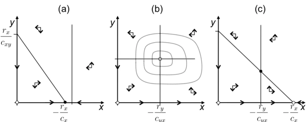
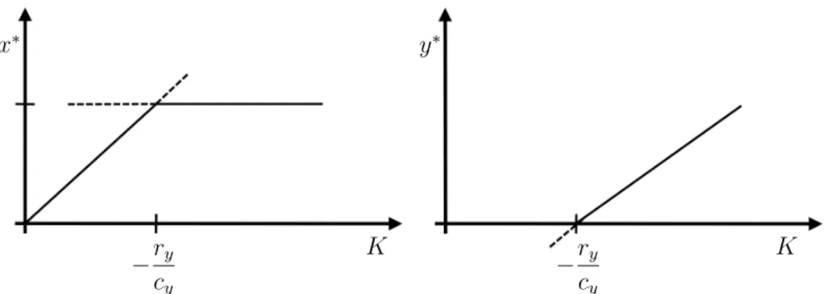
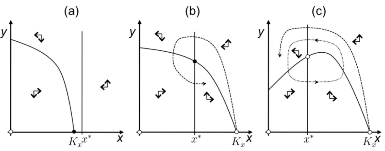
• How does the dynamics depend on the mosquito density α? Draw a figure for the equilibriap∗ as a function of α.
• What are the prospects for getting rid of the disease without getting rid of Anopheles?
We have
˙
p=αp(1−p)−µp= (α−µ)p
1− p
(α−µ)/α
. (20)
For α > µ, this is the dynamics of logistic growth with r = α−µ and K = (α−µ)/α.
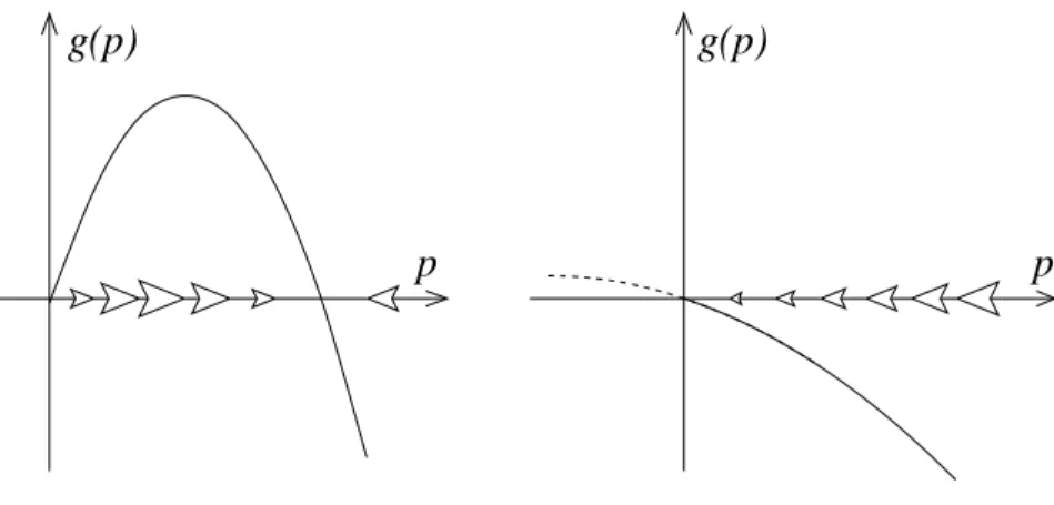
We then get a stable equilibrium of infected people at the carrying capacity K. This is the so-called endemic equilibrium. In contrast, for α < µ, we have a stable equilibrium at p= 0. The disease is extinct although the mosquitoes are still there at some density. Sir Ronald Ross always considered his mathematical models his most important contribution
g(p) g(p)
p p
Figure 2: Phase-line diagram for the infection model (20). Left: α > µ, right: α < µ.
to science! Only very few of his contemporaries understood and appreciated these models.
Only two decades after his death, people started to construct mathematical models for infection and disease in his tradition. For malaria, the qualitative finding that the disease cannot persist with a low mosquito density is confirmed (e.g., parts of USA and Italy). Of course, modern models used in the fight against malaria in Africa and Asia are many levels more complex.
1.5 Bifurcations
For qualitative analysis, it is often of central interest how the equilibrium structure of a model changes if we change some of the model parameters. As a consequence, new equilibria may be created or old ones destroyed, or equilibria may collide and exchange their stability. The resulting qualitative changes in the behavior of the dynamical systems are called bifurcations. We can visualize this “dynamics of the equilibria” in a so-called bifurcation diagram. In the malaria example above, we haveα as a model parameter and the following equilibria: p∗1(α) = 0 and p∗2(α) = K = 1−µ/α. This corresponds to a so- called transcritical bifurcation. We consider a “sufficiently smooth” (at least continuously differentiable) function f(N). The basic types of bifurcations in one dimension are the following:
1. Transcritical bifurcation: two equilibria cross and exchange stability properties. The normal form of a transcritical bifurcation at x = 0 (think of x = N −N∗) and perturbation parameter α reads
˙
x=αx−x2. (21)
2. Saddle-node bifurcation: two equilibria (with opposite stability) collide and vanish (or vice-versa), e.g.,
˙
x=α−x2. (22)
3. Pitchfork bifurcation: three equilibria collide. There are two possibilities. For the supercritical case, the three equilibria are stable – unstable – stable and turn into a stable equilibrium, e.g.,
˙
x=αx−x3. (23)
For the subcritical case, the three equilibria are unstable – stable – unstable and turn into a single unstable equilibrium,
˙
x=αx+x3. (24)
4. Higher-order bifurcations with four or more equilibria colliding are in principle pos- sible, but non-generic.
5. In addition to bifurcations, equilibria can also enter or leave the biological state space.
For a population density N the critical boundary is usually at N = 0. Equilibria can also emerge (or vanish) from infinity. However, most biologically relevant models have limN→∞f(N)<< 0, in which case this is not possible.
1.6 Exercise 1: Harvest models
Consider a population of fish with dynamics according to logistic growth. We want to use this population as a resource and we are looking for a harvesting strategy that guarantees large and stable yield. We consider the following two strategies:
1. With constant-rate harvesting (e.g., because of fishing quota), we have N˙ =rN
1− N K
−H . (25)
2. With relative-rate harvesting, we will catch fish proportional to the stock size, N˙ =rN
1− N K
−EN, (26) where E measures the fishing effort (this could be a quota on fishing boats).
We define the maximum sustainable yield (MSY) as the largest yield that can be taken from the species’ stock over an infinite period.
• Make a bifurcation analysis for both harvesting strategies with H and E as param- eters (diagrams and formulas for bifurcation points). What kinds of bifurcations occur?
• What is the MSY and for which parameter values of H and E do we get this yield?
Which implications for harvesting strategies do you see?
From the solution we see that constant rate harvesting at MSY is dangerous, since any higher rate can lead to a collapsing fish population. With relative rate harvesting, the risk of a sudden crash is avoided. Here, we get the maximal cumulative yield for an intermediate cumulative effort E. It is interesting to consider a situation where multiple fisheries (or countries) compete and try to maximize their share of the harvest. In many cases, we will find that theindividualyield increases monotonically with theindividualeffort – although the cumulative yield decreases. This is an example of the so-called “tragedy of the commons” (see lecture on game theory).
Allee effect In the models we have considered so far, the per-capita growth rateg(N) = N /N˙ was either independent of N (as in exponential growth) or decreased with increasing N (as in logistic growth). In some species, however, the per-capita growth rate is reduced at small population densities, for example because individuals have difficulty finding mates, because group defense (like swarming) or hunting do not work properly, or because of increased predation pressure. Formally, a population experiences a demographic Allee effect if limN→0dg/dN > 0. If the reduction in per-capita growth rate at small densities is so strong that populations below a certain critical density have a negative per-capita growth rate, we say that there is a strong demographic Allee effect. Otherwise the Allee effect is called weak and small populations can still grow. A typical model with strong Allee effect reads
N˙ =rN N
K0 −1
1− N K
, (27)
where K0 < K defines the critical density for which growth becomes positive.
• We can consider relative-rate harvesting on such a population, i.e., N˙ =rNN
K0 −1 1−N
K
−EN. (28) We get equilibria at N = 0 and at the solutions ofE =r((N/K0)−1)(1−(N/K)).
A bifurcation analysis reveals that an allee effect can lead to qualitative changes in the dynamics (see exercises).
1.7 Nondimensionalization
Understanding the qualitative behavior of a model with several parameters can be difficult.
If we vary one parameter at a time while fixing the other parameters at certain values, we cannot be sure that we get the full picture of the model’s behavior. Fortunately, often the only quantity that matters is the relative magnitude of parameters. This is exploited by a model simplification technique called nondimensionalization. The idea is to rescale variables and time such that the rescaled model has fewer parameters but maintains all other model features. As an example, we will nondimensionalize the Allee effect model (27) above. First, we rescale population size by expressing it relative to the carrying capacity K (scaling by K0 would work as well). Now our new variable is x = N/K. Second, we
define a new time scale ˜t =r·t, i.e. rate r on the original time scale corresponds to rate 1 on the new time scale.
With this, we get the new differential equation dx
dt˜= dx dt ·dt
d˜t = 1 Kr
dN
dt =x(1−x) Kx
K0 −1
. (29)
We set k0 =K0/K and drop the tilde (keeping in mind the difference in time scale):
˙
x=x(1−x) x
k0 −1
. (30)
Our new model has just one parameter, which makes the computation of equilibria, bi- furcation analyses etc. more transparent. After we have completed our analyses, we can translate the results back to the original scale. This is especially important if we want to relate them to biological data.
1.8 Bifurcations and structural stability
We have seen that for relative-rate harvesting the inclusion of the Allee effect transforms a transcritical bifurcation into a saddle-node bifurcation. This is indeed typical: Consider a small constant perturbation to a transcritical bifurcation, i.e.,
˙
x=αx−x2+ . (31)
There are equilibria for 1/2(α±√
α2+ 4). We see that there is no bifurcation for >0, because the equilibria never cross. And there are two saddle-node bifurcations for < 0, where there is no equilibrium at all for |α|<2√
−. In an extended parameter space with two perturbation parameters α and , the transcritical bifurcation will only be seen on a low-dimensional manifold (for= 0). [In dynamical systems theory, this kind of analysis is called an “unfolding” of a bifurcation.] We say, the transcritical bifurcation is structurally unstable with respect to constant perturbations. There is a similar effect for the pitchfork bifurcation, but not for the saddle-node bifurcation. In this sense, saddle-node bifurcations represent the most “generic” bifurcation type in one dimension.
1.9 Functional response
Define the functional response F(N): the per capita resource consumption as a function of resource density N per unit time. We set
F(N) = Ts·eN
Ts+Th (32)
where Ts is the time spent searching for food, e the search efficiency, and Th the handling time, i.e., the time needed to process all the attacked prey items. With Th = eN Ts ·th, where th is the time needed to process a single prey item, we get
F(N) = eN
1 +eN th . (33)
After Holling, we can distinguish three types of feeders
1. th = 0: Type 1 functional response, e.g. for filter feeders.
2. th >0: Type 2 functional response, with asymptote at 1/th.
3. th >0 and e=e(N) =e0N: Type 3 functional response. Here, the search efficiency increases with the prey density, for example because a search image is created as the predator get “practice”. This type of functional response is often assumed for higher organisms like vertebrates.
Based on these functional responses, we can now consider the resource dynamics as a function of the consumer density. For the type 1 functional response, this coincides with the relative-rate harvesting model. For type 2 or type 3, we obtain a different behavior.
Resource dynamics for type 2 functional response Consider a model for a resource population with logistic growth, a constant consumer density C, and type 2 functional response:
N˙ =rN 1− N
K
− CeN
1 +ethN. (34)
• Explore the model by plotting Eq. (34) for different parameter combinations.
• Set r = 0.1, K = 1000, th = 0.25, e= 0.05. Make a graphical bifurcation analysis for C. If you want, you can use mathematica, R, maple or some other software package.
• For which consumer densitiesC does the resource experience an Allee effect? Is the Allee effect weak or strong?
Resource dynamics for type 3 functional response For a type 3 response, the model looks as follows:
N˙ =rN 1− N
K
− CgN2
N02+N2 (35)
where C is the number of consumers, g the asymptote of the response curve, and N0 the half saturation point. We may, for example, think ofCas the number of sheep on a meadow and N as the grass biomass. We can analyze this case qualitatively purely graphically.
Take-home message from bifurcation theory Small changes can have a large effect.
This is typical for ecosystems, where these abrupt shifts are frequently seen. The fact that continuous change may lead to discontinuous consequences is counterintuitive for most people. This can have dangerous consequences. Providing insight into the bifurcation structure of natural systems is one of the most important tasks of theoretical ecology.
Examples:
• Fisheries: extinction risk because of overfishing.
• Grasslands turning into deserts because of overgrazing. Very difficult to revert after erosion of top soil.
Of course, it will often be difficult to obtain quantitative estimates of the positions of bi- furcation points. Note also that natural systems exhibit environmental and demographic stochasticity. For this reason, it will be wise to stay at a safety distance from any catas- trophic bifurcation point.
1.10 Stability revisited
We have seen that for asymptotically stable equilibria the population will return to the equilibrium after a single and “sufficiently small” disturbance. However, disturbances in biology are frequent and not necessarily small. How can we deal with this problem? We will treat the case that perturbations are still small, but can be frequent. The relevant question for a second (and each further) perturbation is whether the system has already returned to the equilibrium after the previous perturbation. With a small perturbation N(0) =N∗+δ, we can linearize the dynamics around N∗,
N˙(t)≈Λ(N∗−N(t)) (36)
with
Λ =−∂f(N)
∂N N=N∗
. (37)
For an asymptotically stable equilibrium, we have Λ > 0. Now, Eq. (36) is precisely the dynamics of an immigration-death model (see above) and can be solved exactly. We get
N(t) = N∗ +δexp[−Λt]. (38)
We thus obtain an exponential return to the equilibrium with rate given by Λ. We can define a characteristic return time to the equilibrium as
TR= 1
Λ. (39)
For t TR we will be close to N∗, for t TR, we are still about a distance δ away. We can now compare TR with the average time TD between disturbances. For TR < TD, the system is stable and will remain in the neighborhood of N∗. In contrast, forTD < TR, we get larger excursions away from N∗. In this case, the exact behavior cannot be predicted anymore from a local analysis alone.
1.11 Systems with time delay
One-dimensional autonomous ODE models have a simple equilibrium structure: only stable or unstable equilibrium points can occur. Stable equilibria have simple intervals as domains of attraction. In particular, there are no oscillations or chaotic behavior. All this quickly
changes if the dynamics of a focal population can depend on other factors than just its current size. As already mentioned, ˙N could depend explicitly on time (non-autonomous systems), or on the dynamics of a different population (multidimensional ODEs). As yet another possibility, we consider the following dynamics of a population with damped oscillations:
N(t) =N∗+ (N0−N∗) cos[γt]·exp[−dt]. (40) We then have
N˙(t) = (N0−N∗) exp[−dt] (−γsin(γt)−dcos(γt)) (41)
= (N0−N∗) exp[−dt] (γcos[γ(t−3π/2γ)]−dcos(γt)). (42) With τ = 3π/2γ and using Eq. (40) to solve for and substitute cos[γ(t− 3π/2γ)] and cos(γt), we obtain
N˙(t) = γexp[−dτ]N(t−τ)−dN(t) + (d−γexp[−dτ])N∗. (43) Although ˙N(t) only depends on the size of the focal population, it is not only its current size, but also the size at some earlier time t−τ. Defining b := γexp[−dτ], we recognize this as a time delay in the effect of birth events. Biologically, this can easily be understood if N measures adult individuals, and if it takes some time for juveniles to grow up to reproductive age. There is a lot of theory on ODE’s with time delay (also called difference- differential equations), but analytical results are sparse. Formally, these equations are equivalent to infinite-order ODE’s, which depend on initial conditions on a whole time interval. The math gets quite complex. Nevertheless, delay effects can obviously be relevant in biological systems. If this is the case, they need to be included into a model. As it turns out, however, this is most easily done in a discrete time model using difference equations.
Further example: Lagged logistic growth We can also introduce a time-lag into the logistic growth model, e.g., if the negative feedback of the population density on population growth is not immediate, but only sets in once individuals have grown up. For a lag time τ we get
N˙(t) =rN(t)
1− N(t−τ) K
. (44)
There is no analytical solution of this ODE, but we can study its behavior numerically.
• Use the ”Populus” software to plot numerical solutions for the lagged logistic model (single species/density-dependent growth). Which types of behaviors do you get when you vary the model parameters?
2 One-dimensional models in discrete time
So far, we have assumed that demographic events happen continuously over time and can thus be written as rates. For many biological species with overlapping generations
and continuous reproduction this is a valid approximation. However, many other popula- tions, like annual plants, have discrete generations and many species have clearly defined breeding seasons. These are better modeled in a discrete time framework. More funda- mentally, we have already discussed that the effect of biological events (like birth) on the population dynamics is often not immediate as it is assumed in an ODE system, but only becomes apparent after some time delay. While in continuous time this leads to complex difference-differential equations, effects of time delay (by one time unit or generation) are automatically included in discrete time models. In this section, we will consider a popula- tion with dynamics given by the following first-order, autonomous (= constant coefficient) difference equation,
Nt+1 =F(Nt), t∈N. (45)
An initial value N0 is specified and the reproduction function F can take any shape. The simplest example is the linear difference equation
Nt+1 =F Nt (46)
of geometric growth (for F > 1) or decline (for 0 < F < 1). Geometric growth has the explicit solution
Nt=FtN0. (47)
Very few other discrete time systems have explicit solutions. Next, we need to include density-dependent population regulation. Rather than “dropping down” a model, we want to construct a model from biological principles.
2.1 Non-linear discrete population growth
Consider a fish population of adult stock size Nt. From one breading season to the next (t tot+1), the survival probability for any adult is given bys. (Fors= 0, we have the special case of no generation overlap). During breeding season, the adults produce a number of Lt = bNt larvae. We assume that larvae grow up to reproductive age during one season.
Surviving larvae are recruited to the adult population. We thus need a model for larval survival.
1. Assume that the larvaeLdevelop according to (continuous time) logistic decline, i.e.,
∂Lt(τ)
∂τ =−m1Lt(τ)−m2L2t(τ), (48) wherem1 measures mortality due to extrinsic (e.g. abiotic) factors andm2the density dependent component (e.g., due to competition for resources). WithLt(0) =bNtand a time ∆ between seasons we get
Lt(∆) = bNtm1
(bNtm2 +m1) exp[m1∆]−bNtm2 . (49)
We thus get
Nt+1 =sNt+Lt(∆) =sNt+ c1Nt
1 +c2Nt (50)
with positive constants
c1 =bexp[−m1∆] , c2 =b m2
m1 (1−exp[−m1∆])
This is the Beverton-Holt model for stock recruitment. For s = 0, the model is also called the Verhulst model.
2. An alternative approach assumes that larvae (or juveniles) do not compete primarily among themselves, but with their adult conspecifics. This will be true, in particular, if adult fish eat eggs and larvae of their own species (which is indeed true for many species, where predation is purely size-dependent). We then get
∂Lt(τ)
∂τ =−m1Lt(τ)−m2NtLt(τ), (51) which simply results in
Lt(∆) =bNtexp[−(m1+m2Nt)∆]. (52) We then get a so-calledRicker model for stock recruitment
Nt+1=sNt+Ntexp[r(1−Nt/K)] (53) with constants
r = log[b]−m1∆ , K = log[b]−m1∆ m2∆ .
3. Finally, we can assume that density-dependent competition is entirely among adults (e.g. for breeding places). Then we get a discretized version of logistic growth
Nt+1 =rNt
1−Nt K
, (54)
wherer=s+baccounts for the surviving adult and juvenile individuals from the previous generation.
Recruitment in the Beverton-Holt model is called normal compensation. It increases monotonically with stock size and reaches an asymptote forNt→ ∞ atLmax(∆) =c1/c2. In contrast, recruitment for the Ricker model is over-compensating. Here, Lmax(∆) runs through an intermediate maximum and approaches zero for Nt → ∞. As a consequence, the reproduction function of the Ricker model is usually non-monotonic. The same holds true for the discrete logistic growth model. All three models can be derived in many different ways and for various underlying mechanisms. They are archetypical models of theoretical ecology.
2.2 Discrete versions of continuous models
One special application of discrete models consists simply of an observation in discrete time intervals of a population with continuous birth and death. Thus, we simply set Nt =N(t·∆). An explicit reproduction function can be derived if and only if the ODE can be solved. For logistic growth, in particular, we obtain
Nt+1 = K
1−(1−K/Nt) exp[−r] = λNt
1 + (λ−1)Nt/K (55)
with λ = exp[r]. We recognize this as a special case of the Beverton-Holt model with s= 0, c1 =λ, andc2 = (λ−1)/K. Note that we do not get the discrete logistic growth as the corresponding model. This correspondence also implies that the Beverton-Holt model (withs = 0) is explicitly solvable. In more general, we can define a corresponding discrete model for every autonomous ODE model. The converse is not true, however. In this sense, there are “more” discrete models than continuous models. As we will see, they also show a larger variety of phenomena.
2.3 Equilibria and Stability of Discrete Dynamics
Consider a general discrete dynamical system (1-dim., etc) with continuously differentiable reproduction function,
Nt+1 =F(Nt) ; F0(N) := ∂F(N)
∂N continuous (56)
We can then characterize equilibria as follows
1. Equilibria (or fixed points) of the dynamics are all intersections of the reproduction function with Id(N) (the identity line with slope 1),
F(N∗) = N∗ (57)
2. Let
Λ := ∂F(N)
∂N N∗
.
ThenN∗is locally (asymptotically) stable for|Λ|<1 and locally unstable for|Λ|>1.
Proof: Consider some starting value N0 close to an equilibrium point N∗. Due to the mean value theorem, there is a c∈(N0, N∗) such that
∂F(N)
∂N N=c
= F(N0)−F(N∗)
N0−N∗ = F(N0)−N∗ N0−N∗ . Since the derivative of F(N) is continuous, we have
∂F(N)
∂N c
<1
if |Λ|<1, and thus |F(N0)−N∗|<|N0−N∗|. We thus get a sequenceNi that converges to the equilibrium pointN∗. Similarly, we are (locally) driven away from the optimum for
|Λ|>1.
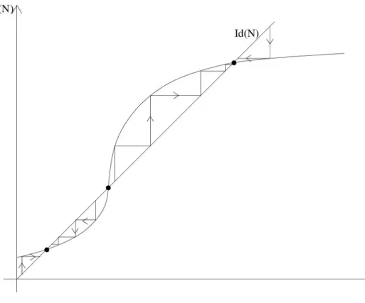
Figure 3: Cobwebbing method to determine the stability of equilibria.
Cobwebbing We can represent the discrete dynamics easily using the cobwebbing method:
• Start at N0, go (vertically) to F(N0).
• Project (horizontally) to the identity line Id(N) to getN1 =F(N0).
• Go vertically toF(N1) and iterate.
Depending on the slope Λ near an equilibrium point, we get four types of characteristic behavior.
1. 0 <Λ<1: monotone convergence.
2. −1<Λ<0: oscillating convergence (damped oscillations) 3. Λ>1: monotone divergence
4. Λ<−1: oscillating divergence (driven oscillations)
2.4 Analysis of the Beverton-Holt and the Ricker model
Beverton Holt model Consider the dynamics of the Beverton-Holt model defined by Nt+1 =F(Nt) = sNt+ c1Nt
1 +c2Nt. (58)
• We have
N(1−s)(1 +c2N) =c1N and thus N1∗ = 0 and
N2∗ = c1 −1 +s c2(1−s)
• With
F0(N) = ∂F(N)
∂N =s+ c1
(1 +c2N)2 ≤s+c1 =F0(0) and F0(N2∗) = s+ (1+(c c1
1−1+s)/(1−s))2 = 1 + (1−s)(1−s−c1)
c1 < 1 for s+c1 > 1 and thus N2∗ > 0. We get monotonic approach of N2∗ for s+c1 >1 and monotonic approach of N1∗ = 0 otherwise.
Lemma In general, if F(N) is continuous and monotonic on a closed interval I ⊆ R+ (e.g., I = [0,∞)) with F(I)⊆I, then every sequence Ni =Fi(N0) with N0 ∈I converges monotonically to a fixed point of F or to ∞.
Proof For F(N0) > N0, we have F(F(N0)) ≥ F(N0) because of monotony, and thus N0 < F(N0) ≤F(F(N0))≤ .... The sequence will either converge to some N∗ or diverge to infinity. In the former case, we have F(N∗) = N∗ since F is continuous. The case F(N0)< N0 works analogously, F(N0) =N0 is trivial.
Ricker model Consider now the Ricker model (we use s= 0, without restriction under rescaling),
Nt+1 =F(Nt) =Ntexp[r(1−Nt/K)]. (59)
• We obtain equilibria at N1∗ = 0 andN2∗ =K.
• We have
F0(N) =
1− N r K
exp[r(1−N/K)]. and thus
Λ1 =F0(0) = exp[r]>1, (60)
Λ2 =F0(K) = 1−r. (61)
• We have a unique maximum of F(N) at Nmax = K/r (and, of course a minimum Nmin = 0).
We thus can distinguish three dynamical regimes (see, for example, Populus, density- dependent population growth, “discrete logistic” = Ricker)
1. For r < 1, the interval I = [0, Nmax] contains both equilibrium points. Since we have F(N) monotonically increasing in I, with F(I) ⊆ I, we obtain monotonic convergence to the stable equilibriumN2∗ =K for every start valueN0 ∈I. For start values N0 ∈/ I, we have F(N0)∈I and the same applies after the first step.
2. For 1 < r <2, we have no longer monotonic convergence, but still |Λ2|<1. Hence, N2∗ =K is still asymptotically stable and approached by damped oscillations.
3. For r >2, we have|Λ2|>1 and therefore do no longer have a stable equilibrium. In particular, we get oscillating divergence for the equilibrium at N2∗ = K. Since the Ricker model has a finite maximum population size, we can ask what happens.
2.5 Limit cycles
The basic idea to gain further insights of the long-term dynamics of the Ricker model and similar systems is to consider the iterated map
F(2)(N) = F(F(N)) resp. F(k)(N) = F(. . . F(F(N))) k−fold (62) across k seasons. Obviously, this is again a discrete dynamical system and can be studied in the same way as the original one. Concerning its long-term behavior, we observe the following elementary facts:
1. Equilibria of F are also equilibria of F(2) and of every higher iteration F(k). 2. For the derivative of F(2) at the fixed points, we have, using the chain rule,
∂F(2)(N)
∂N = ∂F(Z)
∂Z
Z=F(N)· ∂F(N)
∂N . (63)
and accordingly iterated for F(k). For equilibria N∗ of F(N), in particular, this means
∂F(k)(N)
∂N N=N∗
=
∂F(N)
∂N N=N∗
k
. (64)
Thus, stable equilibria of F remain stable for all higher iterations, and unstable equilibria remain unstable.
3. Additional (stable or unstable) equilibria of iterated maps F(k) can occur if the original dynamics F leads to cycling.
Definition and basic properties: Limit Cycles
1. A point N0 is called a point of period k or a k-cycle point if it is a fixed point (equilibrium) of the k-fold iterated map F(k)(N), but not a fixed point of any map F(k0) with 1≤k0 < k. Its orbit
{N0, F(N0), . . . , F(k−1)(N0)}=:{N0, N1, . . . , Nk−1}
is called the corresponding k-cycle. Note that all points Ni in the cycle are fixed points of F(k).
2. A limit cycle is asymptotically stable, if and only if the corresponding cycle points are asymptotically stable equilibria of the k-fold mapping. In particular, we obtain via the chain rule
Λ(k) = ∂F(k)
∂N =
k−1
Y
i=0
∂F(N)
∂N N=Ni
(65) for the derivative ofF(k) at all points of the cycle. The cycle and the corresponding fixed points of F(k) are asymptotically stable if |Λ(k)|<1 and unstable if |Λ(k)|>1.
3. We define the characteristic exponent (or Floquet exponent) λ= 1
k log Λ(k)
= 1
k
k−1
X
i=0
log
∂F(N)
∂N N=Ni
. (66)
Obviously, the cycle is stable for λ <0 and unstable for λ >0.
2.6 Example: Discrete logistic growth
As an example, we consider logistic growth
Nt+1 =F(Nt) = rNt
1− Nt K
, (67)
which behaves similar as the Ricker equation, but is easier to analyze. We have a maximum of F(N) at N =K/2, where F(K/2) = rK/4. There are two equilibria at N1∗ = 0 and at N2∗ =K(r−1)/r. With F0(N) = r(1−2N/K), we obtain F0(0) =r and F0(N2∗) = 2−r.
1. For 0< r <1, we have a single stable equilibrium atN1∗ = 0 and the population dies out.
2. For 1< r <3, a second equilibrium N2∗ appears and is stable, whileN1∗ is unstable.
Approach to the stable equilibrium is monotonic for r <2 and oscillating for r >2.
3. For r >3, both equilibria N1∗ and N2∗ are unstable and we can expect limit cycles or other types of limit behavior.
Finally, for a reasonable biological model, r should not be larger than 4 since otherwise F(N) can get larger thanK and then negative in the next iteration. To study the dynamics via iterated maps, assume K = 1 for simplicity. We then obtain:
F(N) =rN(1−N) (68)
F(2)(N) =r(rN(1−N))(1−rN(1−N)) =r2N(1−N)(1−rN +rN2) (69)
∂F(2)(N)
∂N =r 1−2rN(1−N)
r(1−2N) (70)
(Note that, in general, we have the symmetry F(k)(1−N) =F(k)(N).) We find equilibria F(2)(N) =N for
N1∗ = 0 , N2∗ = r−1
r , N3,4∗ = 1 +r±p
(r−1)2−4
2r (71)
Obviously,N3,4∗ exist forr ≥3. We also find thatF(N3∗) = N4∗and vice-versaF(N4∗) = N3∗. The corresponding derivatives are
Λ(2)1 =r2 Λ(2)2 = (2−r)2 , Λ(2)3,4 = 4 + 2r−r2 (72)
• At r = 3, we have N2∗ = N3∗ = N4∗. We see that, by increasing r beyond this threshold, the previously stable equilibrium N2∗ turns unstable. At the same time two new equilibria of F(2)(N), N3∗ and N4∗, appear and are stable: |Λ(2)3,4| < 1 for 3< r < 1 +√
6 ≈3.45. This is the typical signature of a pitchfork bifurcation. For the original mapF(N), the number of equilibria does not change. The new equilibria for F(2) correspond to a stable limit cycle with period 2.
• For r > 1 +√
6 ≈ 3.45, we have Λ(2)3,4 < −1 and the equilibria N3∗ and N4∗ of F(2) turn unstable. For the iterated mapF(4) this means that the slope at both equilibria increases to (Λ(2)3,4)2 > 1, thereby generating, once again, two new equilibria in a pitchfork bifurcation. We thus obtain a 2-cycle for F(2), corresponding to a 4-cycle for F(N), in each case. In general, every time when a stable equilibrium of F(k) becomes unstable, we get two new stable equilibria of F(2k), and thus a limit cycle with the period 2k. This is the so-called period doubling cascade of the logistic map and many similar discrete maps (such as the Ricker model).
2.7 Bifurcations for discrete time dynamics
We have encountered several cases of bifurcations in the examples, where fixed points originate or disappear or change their stability. They can be summarized as follows. First, the same three types of bifurcations that exist for the continuous time dynamics, ˙N =f(N), also exist in discrete time with iteration function Nt+1 = F(Nt). Instead of the zeros of f(N), we now need to consider the zeros of F(N)−N. We obtain a
• transcritical bifurcation if two zeros of F(N)−N cross and the corresponding fixed points exchange stability (e.g. Beverton Holt model for s+c1 = 1);
• saddle node bifurcationif two fixed points (one stable, one unstable) are either newly generated or annihilated. This happens if Id(N) is tangent to F(N) andF(N) then either crosses or moves away from this line;
• pitchfork bifurcationif a single fixed point splits into three fixed points or, vice-versa, if three fixed points merge and a single one remains (e.g. bifurcation atr = 3 for the iterated logistic map F(2)).
All these bifurcations readily occur also for monotonically increasing iteration functions F(N). With decreasing F(N), another type of bifurcation is possible when a fixed point becomes unstable asF0(N) drops below−1. As described for the logistic map, this typically leads to a pitchfork bifurcation forF(2). ForF(N), it leads to a (stable) limit cycle instead of a single fixed point. This type of bifurcation that cannot occur in the continuous time dynamics. More generally, we call it a
• period doubling bifurcation if a stable fixed point or an existing stable limit cycle becomes unstable and a new stable limit cycle (with a period of double length) emerges.
2.8 Chaos
For the logistic map, we get a series of critical values r2k (withr2 = 3 andr4 = 1 +√ 6≈ 3.45), above which stable cycles of period 2k exist. As it turns out, this sequence of period doubling bifurcation points quickly converges to a finite value rc=r∞ ≈3.57. We can ask what happens beyond this point. As an example, we can consider the logistic map with r= 4 and dissect the interval [0,1] as follows
1. Two intervals I0 = [0,1/2] and I1 = [1/2,1]. Both intervals are mapped by F(N) to the full domain [0,1].
2. Dissect I0 such that I00 = [0, q] is mapped by F to I0 and I01 = [q,1/2] is mapped toI1. Similarly, dissect I1 into I10 and I11.
3. Iterate this: I000 ⊂I00 is mapped byF toI00 and byF(2) toI0;I001 ⊂I00is mapped toI01 and then toI1, etc. In general,Ii0i1i2...ik ⊂Ii0 withij ∈ {0,1} is mapped by F toIi1i2...ik ⊂Ii1 and byF(k) to Iik.
4. In general, if (e.g.) N ∈I0100, then N ∈I0, F(N) ∈I1, F(2)(N) ∈I0, F(3)(N)∈ I0. We can identify each point with an infinite interval nesting (dyadic transformation).
5. Points with periodic nesting correspond to periodic orbits. There are points with ev- ery period, starting withI0000...and I1111..., which encode the (unstable) fixed points.
6. All points on interval boundaries are attracted by 0 (dense set: population on the verge of extinction; this is special for r= 4).
7. Almost all points (with no period in the nesting) must have orbits of infinite length.
We also see that orbits of very close points can differ widely after even a few gener- ations. This is the signature of chaos.
8. For the special case r= 4, there is an explicit solution for the dynamics Nk= sin2[2k−1πθ] where θ = 1
π sin−1[N01/2]. (73) We see that we get aperiodic orbits for all irrational θ.
These observed phenomena are not specific tor = 4, but occur for most valuesr > rc. We can summarize them as follows:
• There are infinitely many periodic points, with all kinds of periods, even and odd.
• For most r values, we obtain chaos, indicated by orbits of infinite length that never come back to a starting point. Another characteristic of chaotic solutions is that very small initial differences are magnified due to the mapping. This means that the long-term predictability of the system gets lost (butterfly effect).
• As analog to the Floquet exponent for finite cycles, one defines theLyapunov exponent λ= lim
k→∞
1 k
k−1
X
i=0
log
∂F(N)
∂N N=Ni
(74) for any point N0 with infinite orbit. A positive Lyapunov exponent indicates that small initial differences are magnified and the resulting orbit is chaotic.
• The chaotic regimes are interlaced by intervals with stable limit cycles with low period (e.g. 3-cycles).
Periodicity and Chaos in Biology Our examples show that even very simple models (in one dimension!) can give rise to very complex phenomena. Periodic dynamics are a frequent observation in biology, also in population dynamics. There can be multiple causes for such cycles. With discrete dynamics, cycling is created by an overshooting of the equi- librium, which is typical of many systems where regulation is not immediately effective, but acts with a certain delay. Essentially the same behavior is seen in continuous delay ODE’s. Chaotic behavior in biology has been speculated a lot. From a theoretical point of view, we should expect chaos in particular for systems with higher dimension (multi- ple interacting species). Even with continuous dynamics, chaos exists in dimension ≥ 3.
However, convincing empirical evidence is hard to obtain. In particular, it is often difficult (or impossible) to distinguish long cycles and/or stochastic noise from “real” deterministic chaos. Finally, true chaos is never strictly possible in populations with a discrete number of individuals. Nevertheless, chaos is a field where biology has inspired mathematics and has helped to found chaos theory as a research field (Robert May 1974, 1976).