The Asia Financial Crises and Exchange Rates: Had there been volatility shifts for Asian currencies?

IHS Economics Series Working Paper 254

September 2010

The Asia Financial Crises and Exchange Rates: Had there been volatility shifts for Asian currencies?

Takashi Oga

Wolfgang Polasek

Impressum Author(s):

Takashi Oga, Wolfgang Polasek Title:

The Asia Financial Crises and Exchange Rates: Had there been volatility shifts for Asian currencies?

ISSN: Unspecified

2010 Institut für Höhere Studien - Institute for Advanced Studies (IHS) Josefstädter Straße 39, A-1080 Wien

E-Mail: o ce@ihs.ac.at ffi Web: ww w .ihs.ac. a t

All IHS Working Papers are available online: http://irihs. ihs. ac.at/view/ihs_series/

This paper is available for download without charge at:

https://irihs.ihs.ac.at/id/eprint/2013/

The Asia Financial Crises and Exchange Rates:

Had there been volatility shifts for Asian currencies?

Takashi Oga, Wolfgang Polasek

254

Reihe Ökonomie

Economics Series

254 Reihe Ökonomie Economics Series

The Asia Financial Crises and Exchange Rates:

Had there been volatility shifts for Asian currencies?

Takashi Oga, Wolfgang Polasek September 2010

Institut für Höhere Studien (IHS), Wien

Institute for Advanced Studies, Vienna

Contact:

Takashi Oga Chiba University 1-33 Yayoi-Cho

Inage-Ku, Chiba, 263-8522, email: ohga@le.chiba-u.ac.jp

Wolfgang Polasek

Department of Economics and Finance Institute for Advanced Studies Stumpergasse 56

1060 Vienna, Austria

: +43/1/599 91-155 email: polasek@ihs.ac.at

Founded in 1963 by two prominent Austrians living in exile – the sociologist Paul F. Lazarsfeld and the economist Oskar Morgenstern – with the financial support from the Ford Foundation, the Austrian Federal Ministry of Education and the City of Vienna, the Institute for Advanced Studies (IHS) is the first institution for postgraduate education and research in economics and the social sciences in Austria. The Economics Series presents research done at the Department of Economics and Finance and aims to share “work in progress” in a timely way before formal publication. As usual, authors bear full responsibility for the content of their contributions.

Das Institut für Höhere Studien (IHS) wurde im Jahr 1963 von zwei prominenten Exilösterreichern –

dem Soziologen Paul F. Lazarsfeld und dem Ökonomen Oskar Morgenstern – mit Hilfe der Ford-

Stiftung, des Österreichischen Bundesministeriums für Unterricht und der Stadt Wien gegründet und ist

somit die erste nachuniversitäre Lehr- und Forschungsstätte für die Sozial- und Wirtschafts-

wissenschaften in Österreich. Die Reihe Ökonomie bietet Einblick in die Forschungsarbeit der

Abteilung für Ökonomie und Finanzwirtschaft und verfolgt das Ziel, abteilungsinterne

Diskussionsbeiträge einer breiteren fachinternen Öffentlichkeit zugänglich zu machen. Die inhaltliche

Verantwortung für die veröffentlichten Beiträge liegt bei den Autoren und Autorinnen.

Abstract

We analyse the volatility structure of Asian currencies against the U.S. dollar (USD) for the Thai Baht THB, the Philippine Peso PHP, the Indonesian Rupiah IDR and the South Korean Won KRW. Our goal is to check if the characteristics of the volatility dynamics have changed in a K-state switching AR(1)-GARCH(1,1) model in the last decade 1995-2008 covering the Asian crisis. We estimate the model of Haas et al. (2003) with MCMC and we find that for the four currencies the volatility dynamics has changed at least once.

Keywords

Markov switching GARCH models, Asian currency crisis 1997, Volatility breaks, Bayesian MCMC, Model choice

JEL Classification

F31, C11, C22

Contents

1 Introduction 1

2 Model and Bayesian Inference 2

2.1 The Volatility Model ... 2

2.2 The prior and posterior distribution ... 3

2.3 Gibbs sampling ... 4

3 Empirical Analysis 4 3.1 Model choice ... 4

3.2 Thailand ... 5

3.3 The Philippines ... 6

3.4 Indonesia ... 7

3.5 South Korea ... 7

4 Conclusions 7

References 8

The Asia Financial Crises and Exchange Rates 1

1 Introduction

GARCH (generalized autoregressive conditional heteroscedasticity) models of Boller- slev (1986) have become very popular in econometrics to analyze the volatility struc- tures of financial time series. Since the pioneering work of Hamilton (1989), Markov switching models have become a primary tool to analyze break points in time series.

The last decade have seen some financial crises and it is interesting to see if these crises can be detected or are reflected in the volatility structure of exchange rates.

The term financial crisis is applied broadly to a variety of situations in which some financial institutions or assets suddenly loose a large part of their value. The consequences of financial crises can be manifold like banking panics, recessions and currency revaluations or system changes. Other situations that are often called financial crises include stock market crashes and the bursting of financial bubbles, as well as international phenomena like currency crises and sovereign defaults.

In the following we concentrate on volatility changes of four Asian currencies in the period 1995 to 2008, which covers the Asia financial crisis of 1997. Recall that the Asian financial crisis

• has started May 1997 in Thailand,

• had most effects for Thailand, Indonesia and South Korea,

• minor effects for Hong Kong, Malaysia, Laos and Philippines,

• while China, India, Taiwan, Singapore, Vietnam and Japan were less suffering.

The reason why we concentrate on these four currencies is the fact that these cur- rencies gave up their currency pegs in the aftermath of the Asia crisis. Table 1 lists the dates when the four countries changed to a floating system. Note that all these

Table 1. Asian currencies that changed from pegged to floating Thailand July 2, 1997

Philippine July 11, 1997 Indonesia August 14, 1997 South Korea December 16, 1997

four changes occurred in the second half of the financial crisis year 1997. Singapore,

China, Hong Kong and Russia did not change their currency systems following the

Asia crisis, and their currencies were pegged mainly to the USD. Now our question

is: Had the changes in the currency systems been accompanied by similar patterns in

the volatility of the currency returns? If the pegs were abandoned because of specula-

tive attacks, then the time point of the peg change must coincide with a break point in

a volatility model of the currency returns. Can switching econometric models detect

the regime shifts in the volatilities and do the estimated results correspond to the of-

ficial dates? By analysing regime shifts in the volatilities since 1995, an econometric

models could possibly detect other change points that were not necessarily related to

2 Takashi Oga and Wolfgang Polasek

the Asian crisis and might have been there for other reasons. We consider the data for the four currencies that are listed in Table 1: The Thailand Baht THB, the Philip- pine Peso PHP, the Indonesia Rupiah IDR, and the South Korean Won KRW from Jan. 3rd 1995 to mid 2008. We construct a Markov switching AR(1)-GARCH(1,1) model to analyze the structural change in the volatility dynamics and to interpret why the volatility change occurred. From a Bayesian oint of view, we construct a Markov chain Monte Carlo MCMC algorithm to simulate parameter densities and we employ the deviance information criterion DIC for determining the number of the structural changes. Section 2 introduces the AR(1)-GARCH(1,1) model and the Bayesian MCMC approach and Section 3 discusses the empirical results of four cur- rencies: THB, PHP, IDR, and KRW. Conclusions are given in Section 4.

2 Model and Bayesian Inference

2.1 The Volatility Model

We assume a K-state Markov switching model where each component k = 1, · · · , K . is a GARCH model with an AR(1) disturbance. Each component is assumed to have an unconditional mean µ

and AR(1) coefficient φ

:

y

= f

(y

) = µ

+ φ

(y

− µ

) + ε

, ε

∼ N (0, h

). (1) The conditional variance h

for each state k is allowed to change through time by a GARCH(1,1) process:

h

= ω

+ γ

h

+ α

ε

. (2) The discrete random variables s = {s

, · · · , s

, · · · , s

} are the state indicators at time t, and s

∈ {1, · · · , k, · · · , K } follows a Markov process with transition matrix Π with K states

s

∼ M arkov(Π), (3)

and the elements of Π are the probabilities π

of Π and are given by

π

= P (s

= j|s

= i), i = 1, · · · , K, j = 1, · · · , K. (4) As the regime changes, the indicator s

changes from 1 to K in ascending ordering.

Thus, back switching are not allowed and the only non-zero probabilities in Π are the ones of reaching regimes j and j + 1 from state j. Therefore we define for Π a restricted (step-up) transition probability matrix following the approach of Chib (1998). Under these settings, the observation equation is a mixture model

y

=

K

X

k=1

1(s

= k)f

(y

), (5)

where 1(·) is a indicator variable for the event in the parenthesis. If the condition is

true, then the indicator is 1, otherwise zero. The likelihood function is given by

The Asia Financial Crises and Exchange Rates 3

L(y | Θ) = f(y

| Θ

)

T

Y

t=2 K

X

k=1

f(y

| y

, s

= k, Θ)P(s

= k | y

, Π),

= f(ε

|Θ

)

T

Y

t=2 K

X

k=1

f (ε

|I

, Θ

)P (s

= k|I

, Θ) (6) where y = (y

, · · · , y

)

, y

= (y

, · · · , y

)

, I

is the available information set at time t, and Θ = {Θ

, · · · , Θ

, Π}, Θ

is the parameter vector associated with model k, namely (µ

, φ

, ω

, γ

, α

)

.

The components of the likelihood function are f(ε

| Θ

) = 1

q 2π

1

exp



− (y

− µ

)

2

1



 , (7)

f (ε

| I

, Θ

) = 1 p 2πh

exp

− (y

− µ

− φ

(y

− µ

))

2h

. (8) We can evaluate the likelihood function using the GARCH densities as in Hamilton (1989) method independently only under Haas et al.(2003) formulations without any approximations for the GARCH model. This makes the likelihood of the models easy to be evaluated. Because of the non-linearity and the many parameters for large K, classical maximum likelihood methods requiring numerical optimizations are dif- ficult to apply. In this situation, Bayesian MCMC methods yield faster parameter estimates without any optimizations.

2.2 The prior and posterior distribution

Let Θ be the parameter set of the K-state Markov switching model and we assume that the prior for Θ = {Θ

, · · · , Θ

, Π} is block-wise independent:

p(Θ) = p(µ)p(φ)p(θ)

K−1

Y

k=1

p(π

) (9)

with µ = (µ

, µ

, · · · , µ

)

, φ = (φ

, φ

, · · · , φ

)

, θ = (θ

, θ

, · · · , θ

)

, θ

= (ω

, γ

, α

)

, k = 1, ..., K. For the vector of mean coefficients µ we assume

µ ∼ N (µ

, Σ

), µ

= 0

, Σ

= 1000 × I

,

and for the AR(1) coefficients vector φ, we assume an independent uniform prior for each element φ

,

φ

∼ U(−1, 1), k = 1, · · · , K.

To assure stationarity, the prior density is truncated to the interval (−1, 1).

For the prior of the GARCH parameters, we assume a truncated normal density

θ ∼ N (µ

, Σ

), µ

= 0

, Σ

= 1000 × I

4 Takashi Oga and Wolfgang Polasek

where the truncation is implied by imposing positive variances as a condition for the GARCH model and are given for each state i = 1, · · · k by

ω

, γ

, α

> 0, and γ

+ α

< 1,

For the non-zero probabilities elements of the step-up transition matrix we use the beta distribution

π

∼ B(a, b),

and as in Chib (1998) we use the hyper-parameters a = 9, b = 0.1.

The posterior distribution is - by Bayes’s theorem - proportional to multiplying (9) and (6)

f (Θ | y) ∝ L(y | Θ)p(Θ). (10) 2.3 Gibbs sampling

This section develops a MCMC algorithm for the K-state switching AR(1)-GARCH(1,1) model and lists all necessary full conditional distributions for the posterior in (10).

The MCMC sampling scheme with Metropolis-Hastings (MH) steps comprises:

0 Initialize Θ

,

1 draw π

from a beta distribution (see Kim and Nelson (1999)),

2 draw θ using a random walk MH algorithm (see Holloway, Shankar and Rahman (2002)),

3 draw φ using the MH algorithm (see Chib and Greenberg (1995)), 4 draw µ from a normal distribution,

5 draw s from a Bernoulli distribution (see Kim and Nelson (1999)).

We iterate step 1 to 5 for G = 50000 times and we discard 10000 iterations as burn-in.

3 Empirical Analysis

We consider the daily log returns of four Asian currencies against the USD from Jan.

3, 1995 to June 30, 2008: The Thailand’s Baht THB, the Philippine Peso PHP, the Indonesia Rupiah IDR, and the S. Korean Won KRW (with sample sizes 3387, 3152, 3140, and 3390).

3.1 Model choice

To determine the adequate number of regimes K, we calculate the dispersion in-

formation criterion DIC suggested by Spiegelhalter et al.(2002). Table 3.1 lists the

DIC’s for up to K = 1, · · · , 5 regimes. Only for the Thai Baht THB we find 3 struc-

tural changes (as the minimum DIC for K is 4) between 1995 and 2008, while for

the other 3 currencies

The Asia Financial Crises and Exchange Rates 5

Table 2. Model choice by DIC for 5 regimes (minimum DIC in bold)

THB PHP IDR KRW

k = 1 3864.64 2374.26 8079.09 3899.39 k = 2 3682.10 1871.54 7963.10 3822.86 k = 3 3693.61 1855.72 7830.75 3808.48 k = 4 3589.26 2006.95 7986.91 5698.24 k = 5 4022.80 2549.86 7984.27 4470.55

To estimate the exact date of the structural change, we have computed the poste- rior probability of the states s

using s

from the MCMC sample:

P ˆ (s

= i) = G

G

X

g=1

1(s

= i), i = 1, · · · , K.

In the Markov switching model, the state s

is estimated through the largest posterior probability P ˆ (s

= i) and the estimated regime changes are shown in Table 3.1

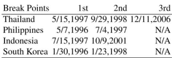
Table 3. Estimated dates of the break points

Break Points 1st 2nd 3rd

Thailand 5/15,1997 9/29,1998 12/11,2006 Philippines 5/7,1996 7/4,1997 N/A Indonesia 7/15,1997 10/9,2001 N/A South Korea 1/30,1996 1/23,1998 N/A

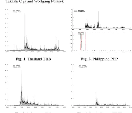
The time series of estimated posterior volatilities and the probability of a break point for the four countries are shown in Figure 1-4.

3.2 Thailand

Our analysis in Figure 1 shows that Thailand’s currency has changed 3 times the volatility regime and Table 3.1 shows that the first break point occurred on May 15, 1997. Recall from Table 1 that the Asia crisis started by serious attacks of hedge funds on May 14 and 15, 1997, against the Thai currency, so the break point marks exactly the beginning of the Asian crisis. After fruitless defenses the authorities had to change the currency system on July 2, 1997, 6 weeks after the attacks began: thus the estimated structural change in volatilities is exactly in line with financial history.

The second break point occurred on Sep. 29, 1998, 5 quarters after the regime switch, and marked the end of the high volatility regime, about 1 month after a new agreement with the IMF had been found.

3

On Oct. 3, 1998, Japan declared “A New Initiative to Overcome the Asian Currency Cri-

sis” (or New Miyazawa Initiative) to help Asian economies and the stability of financial

6 Takashi Oga and Wolfgang Polasek

Fig. 1. Thailand THB Fig. 2. Philippine PHP

Fig. 3. Indonesian IDR Fig. 4. South Korean KRW

The third break point was found in our analysis for Dec. 11, 2006, after which the volatility increased almost to the level of the Asia crises. This increase in volatility was caused by a coup d’etat, which took place on (Tuesday) Sep. 19, 2006, when the Thai army toppled the elected government of Prime Minister Thaksin Shinawatra.

The subsequent instability of the new government of Thailand made the currency more volatile.

3.3 The Philippines

The Philippine currency dynamics changed 2 times according to the estimates of posterior probability in Figure 2. The first break point in the currency volatilities oc- curred on July 11, 1996, 1 year before the Asia crisis and from the estimated volatil- ities we see that the size and duration was negligible compared with the Asia crises.

Table 3.1 shows that the second break point was on July 4, 1997, 2 days after the Thai authorities had to change their currency system. It shows that the currency has become volatile before the currency system changed and as a result the Philippine central bank raised interest rates by 3.75 percentage points in defense of the peso in spring 1997. After the second structural change point, the high PHP currency volatil- ities have continued for a long time and the stabilization worked rather gradually.

markets. Japan provided a package of US$30 billion for the economic recovery in Asia. It

seems that the funding program has helped to stabilize the markets.

The Asia Financial Crises and Exchange Rates 7 3.4 Indonesia

Similar to Thailand, the first break point of the currency volatilities occurred on July 15, 1997, just 1 month before the change in the currency system happened on Aug.

14, 1997, and we see that the volatility of the IDR went up. The next change point is estimated for Oct. 9th, 2001, as can be seen in Figure 3 and Table 3.1. President Abdurrahman Wahid was discharged on July 23, 2001, as he broke with the IMF.

The next president Diah Permata Megawati Setiawati Sukarnoputri, the daughter of the former president Sukarno, restored the relationship between Indonesia and the IMF. After the event, the IMF resumed the financial support for Indonesia on Sep.

10, 2001, and the long 4-year period of high volatilities came to an end. This shows that the restart of the IMF funding policy stabilized the Indonesia IDR despite the coincidence of the 9/11 attacks which had no effects on the Asian currencies.

3.5 South Korea

South Korea’s currency had changed 2 times the currency regime according to the estimates shown in Figure 4. The first change occurred on Jan. 30, 1996, 2 years before the second one, during the peg regime and was quite small. This first sign of trouble in Korea became evident, when the current account deficit widened from 2%

of GNP in 1995 to 5% in 1996. The subsequent change in the currency occurred on Dec. 16, 1997, and was the latest of the four countries considered in this study. This came after some serious drops in the stock markets at the end of the year together with a downgrading from A1 to B2 in Moody’s credit rating.

Table 3.1 shows that the second break point is on January 23, 1998, 1 month after the currency system has changed. Thus the currency became shortly volatile after the change from peg to floating. This raises an interesting issue: Why were there no speculative attacks on the KRW (during 1997) and is this the reason of a delayed volatility response in the currency?

4 Conclusions

This paper has analyzed the structural changes for the volatilities of Asian curren- cies over the 1995-2008 decade covering the Asia and the ”dot.com” crises and the slump following the 9/11 attacks. We find that strong volatility changes had occurred for the Thai THB and Indonesian rupiah that were caused by the Asian financial cri- sis in 1997.

In the introduction we asked the research question: Were the changes in the four

currency systems accompanied by similar patterns in the volatility structure? The

answer is rather no, despite the fact that the four countries changed from peg to float

in the second half of 1997. Vulnerability, duration and the response dates to currency

attacks seem to be quite different and to depend on the underlying strength of the

economies. Occasionally we find similar patterns of currency changes like the one

for Thailand and Indonesia. Furthermore, some regime shifts are strongly related to

8 Takashi Oga and Wolfgang Polasek

the internal politics of the countries, like discharge of presidents or coup d’etat. And we find that quite intensive influence by the IMF or other countries can be an effec- tive way to stabilize the volatility of the currencies.

We find that that the effects of the Asia crises are quite divers if we only concentrate on currency fluctuations. More can be learned if we take into account the effects of the stock markets and interest rates, or growth and deficits. But the modeling com- plexity will not decrease since relationships between countries will not become easier in times of a crisis. But our modeling approach shows that regime shift models can resolve some of the complexities in currency developments and changes in currency regimes that are triggered by crises developments.

References

[1] T. Bollerslev. Generalized Autoregressive Conditional Heteroskedasticity. Jour- nal of Econometrics, 31:307-327, 1986.

[2] S. Chib. Estimation and comparison of multiple change-point models. Journal of Econometrics, 86:221-241, 1998.

[3] S. Chib and E. Greenberg. Understanding the Metropolis-Hastings Algorithm.

American Statistician, 49:327-335, 1995.

[4] M. Haas, S. Mittnik, and M. S. Paolella. A New Approach to Markov-Switching GARCH Models. Journal of Financial Econometrics, 2:495-530, 2004.

[5] J. D. Hamilton. A New Approach to the Econometric Analysis of Nonstationary Time Series and the Business Cycle. Econometrica, 57:357-384, 1989.

[6] G. Holloway, B. Shankar, and S. Rahman. Bayesian Spatial Probit Estimation:

a Primer and and Application to HYV rice adoption. Agricultural Economics, 27:383-402, 2002.

[7] C. Kim and C. R. Nelson. State-Space Models with Markov Switching. The MIT

Press, Cambridge, 1999.

Authors: Takashi Oga, Wolfgang Polasek

Title: The Asia Financial Crises and Exchange Rates: Had there been volatility shifts for Asian currencies?

Reihe Ökonomie / Economics Series 254

Editor: Robert M. Kunst (Econometrics)

Associate Editors: Walter Fisher (Macroeconomics), Klaus Ritzberger (Microeconomics)

ISSN: 1605-7996

© 2010 by the Department of Economics and Finance, Institute for Advanced Studies (IHS),

Stumpergasse 56, A-1060 Vienna   +43 1 59991-0  Fax +43 1 59991-555  http://www.ihs.ac.at

ISSN: 1605-7996