Ancestral Sequence Reconstruction:

(1)

Ancestral Sequence Reconstruction:

Methods and Applications

Dissertation

zur Erlangung des Doktorgrades der Naturwissenschaften (Dr. rer. nat.) der

Fakultät für Biologie und vorklinische Medizin der Universität Regensburg

vorgelegt von

Kristina Straub, geb. Heyn aus Bad Kreuznach

Juni 2018

(2)

(3)

Das Promotionsgesuch wurde eingereicht am: 15.06.2018

Die Arbeit wurde angeleitet von: Prof. Dr. Rainer Merkl

Unterschrift: ...

Kristina Straub

(4)

(5)

Abstract

A major goal in the study of molecular evolution is to elucidate properties of ancestral proteins and to understand their adaption induced by changes in the environment. Due to the lack of macromolecular fossils, ancestral sequence reconstruction (ASR) is the only alternative to de- duce sequences for evolutionary precursors of extant proteins. Within the last years, ancestral proteins were inferred spanning a time-period of more than 3 billion years. Ancestral proteins from eubacteria, archaea, yeast, and vertebrates could be reconstructed. Thus, ASR yielded insights into the early history of life and the evolution of proteins and of macromolecular com- plexes. Moreover, it turned out that ASR is an effiecient method of protein design, because the reconstructed sequences often possess favorable properties like an increased thermostability.

The popularity and efficacy of ASR benefitted from improvements in DNA sequencing technol-

ogy, the enormous rise of computer power and the refinements of algorithms for sequence and

phylogenetic analyses to be seen during the last decades. Thus, elaborated ASR methods are at

hand nowadays that can be applied to a variety of evolutionary problems. For an ASR applica-

tion, the user has however to pick representatives from an overwhelming number of sequences,

which is no trivial task. To advance ASR technology and to assist the user, the first part of this

thesis focusses on the design of a standardized ASR protocol and the development of a novel

filter aimed at facilitating sequence selection. In the second part, ASR is used as a method to

elucidate properties of an ancestral enzyme complex and to identify protein-protein interaction

hotspots.

(6)

(7)

References of Published Manuscripts

This thesis is composed of the following published or accepted manuscripts and one additional chapter, which contains unpublished data:

A Straub, K., Merkl, R. (2018). Ancestral sequence reconstruction as a tool for the elucidation of a stepwise evolutionary adaptation. In Computational Methods in Protein Evolution: Methods and Protocols, Springer, New York. In Press

B Busch, F., Rajendran, C., Heyn, K., Schlee, S., Merkl, R., & Sterner, R. (2016).

Ancestral tryptophan synthase reveals functional sophistication of primordial en- zyme complexes. Cell chemical biology, 23(6), 709-715.

C Holinski, A., Heyn, K., Merkl, R., & Sterner, R. (2017). Combining ancestral se- quence reconstruction with protein design to identify an interface hotspot in a key metabolic enzyme complex. Proteins: Structure, Function, and Bioinformatics, 85(2), 312-321.

In the course of this work, I contributed to further publications, which are not part of this thesis:

D Linde, M., Heyn, K., Merkl, R., Sterner, R., & Babinger, P. (2018). Hexamer- ization of geranylgeranylglyceryl phosphate synthase ensures structural integrity and catalytic activity at high temperatures. Biochemistry, 57(16), 2335-2348.

E Kneuttinger, A.C., Winter, M., Simeth, N.A., Heyn, K., Merkl, R., König, B., Sterner, R. (2018). Artificial light-regulation of an allosteric bi-enzyme complex by a photosensitive ligand. ChemBioChem, published online

F Plössl, K., Schmid, V., Ammon, M., Straub, K., Merkl, R., Weber, B., Friedrich

U. (2018). Pathomechanism of mutated and secreted retinoschisin in X-linked

juvenile retinoschisis. Submitted for Publication

(8)

(9)

Personal Contributions

Publication A

Rainer Merkl and myself designed the protocol. Both authors wrote the manuscript and Fig- ure 2.1 was created by myself.

Publication B

The experiments were conducted by Florian Busch and Sandra Schlee. Chitra Rajendran per- formed crystallisation experiments. Rainer Merkl and myself performed ASR; I generated the figures and tables (Figure 4.5, Figure 4.6, and Table 4.5), analyzed 3D structures and cre- ated the corresponding pictures (Figure 4.3, Figure 4.4, and Figure 4.9). Florian Busch and I drafted the manuscript and I wrote the respective parts of the paper. Rainer Merkl and Reinhard Sterner supervised the research and all authors contributed to writing of the manuscript.

Publication C

The research was designed by all authors. Alexandra Holinski and I contributed equally to this publication: Biochemical experiments were performed by Alexandra Holinski and bioinformatic research was conducted by myself leading to all corresponding figures (Figure 5.2, Figure 5.3, Figure 5.4, Figure 5.5, Figure 5.8, Table 5.2, Table 5.3, Table 5.4, and Table 5.5).

Rainer Merkl and Reinhard Sterner supervised the work; the manuscript was written by all

authors.

(10)

(11)

Abstract v

References of Published Manuscripts vii

Personal Contributions ix

List of Figures xv

List of Tables xvii

1 General Introduction 1

1.1 Evolution in Biology . . . . 1

1.2 Ancestral Sequence Reconstruction . . . . 3

1.3 Aim and Scope of this Work . . . . 7

1.4 Guide to the Following Chapters . . . . 8

2 Ancestral Sequence Reconstruction as a Tool 11 Abstract . . . . 11

2.1 Introduction . . . . 12

2.2 Protocol . . . . 14

2.2.1 Ancestral Sequence Reconstruction . . . . 14

2.2.2 Identification of Specificity-determining Residues by Means of Intermedi- ate Sequences . . . . 16

2.3 Notes . . . . 17

3 Sequence Selection by FITSS4ASR 21 3.1 Introduction . . . . 21

3.2 Results . . . . 23

3.2.1 Criteria Guiding Sequence Selection for ASR . . . . 23

3.2.2 FitSS4ASR: Filtering Sequence Sets for ASR . . . . 24

3.2.3 Choosing a Datasets for ASR . . . . 27

3.2.4 Conventional Sequence Selection for ASR of GGGPS . . . . 27

3.2.5 Sequence Selection by Means of FitSS4ASR for an ASR of GGGPS . . . . 28

(12)

3.3 Discussion . . . . 32

3.3.1 ASR Requires a Strong Phylogenetic Signal Necessitating a Rigorous Pre- selection of Sequences . . . . 32

3.3.2 Future Directions . . . . 33

3.4 Materials and Methods . . . . 33

3.4.1 Conventional ASR Protocol . . . . 33

3.4.2 FitSS4ASR, a Semi-supervised Protocol for Sequence Selection . . . . 33

3.4.3 Indicators of ASR Suitability . . . . 34

3.4.4 Ancestral Sequence Reconstruction . . . . 35

3.5 Supplemental Figures and Tables . . . . 36

4 The Ancient Nature of the Tryptophan Synthase Complex 37 Summary . . . . 37

4.1 Introduction . . . . 38

4.2 Results and Discussion . . . . 39

4.2.1 Sequence Reconstruction of LBCA TS Subunits . . . . 39

4.2.2 Stabilities of LBCA TS Subunits and Subunit Interaction . . . . 40

4.2.3 Crystal Structure and Substrate Channeling of LBCA TS . . . . 40

4.2.4 Impact of the β-subunit for the Catalytic Efficiency of the α-subunit . . . 42

4.2.5 Impact of the α-subunit for the Catalytic Efficiency of the β-subunit . . . 43

4.3 Significance . . . . 44

4.4 Experimental Procedures . . . . 45

4.4.1 Sequence Reconstruction . . . . 45

4.4.2 Cloning and Expression . . . . 45

4.4.3 Absorbance and Circular Dichroism (CD) Spectroscopy . . . . 46

4.4.4 Differential Scanning Calorimetry (DSC) . . . . 46

4.4.5 Analytical Size Exclusion Chromatography . . . . 46

4.4.6 Fluorescence Titration . . . . 47

4.4.7 Transient Kinetics . . . . 47

4.4.8 Steady-state Kinetics . . . . 47

4.4.9 Crystallization and Structure Determination . . . . 48

4.5 Supplemental Figures and Tables . . . . 49

5 Identification of a Protein Interface Hotspot 55 Abstract . . . . 55

5.1 Introduction . . . . 56

5.2 Materials and Methods . . . . 59

5.2.1 Cloning and Mutagenesis of hisF Genes . . . . 59

5.2.2 Heterologous Expression and Purification of HisF Proteins and zmHisH . 60

5.2.3 Fluorescence Titration . . . . 61

(13)

5.2.4 Far-UV CD-Spectroscopy . . . . 61

5.2.5 ASR of Intermediate Sequences . . . . 61

5.2.6 Interface Prediction . . . . 62

5.2.7 Homology Modelling . . . . 62

5.2.8 Calculating the Interaction Energy of Protein Complexes . . . . 62

5.2.9 Predicting Hotspots . . . . 62

5.3 Results . . . . 63

5.4 Discussion . . . . 68

5.5 Supplemental Figures and Tables . . . . 70

6 Comprehensive Summary, Discussion and Outlook 75

Digital Supplemental Data 79

Abbreviations 81

References 85

Acknowledgment 101

(14)

(15)

List of Figures

1.1 Darwin’s sketch of the tree of life . . . . 1

1.2 Tree of life . . . . 2

1.3 “Resurrection” of ancestral proteins based on ASR . . . . 4

1.4 Calculation of a phylogenetic tree . . . . 6

2.1 Identification of specificity-determining residue positions of the HisF:HisH inter- face by means of a vertical approach . . . . 15

3.1 Criteria applied by FitSS4ASR to eliminate sequences . . . . 24

3.2 Workflow of FitSS4ASR . . . . 26

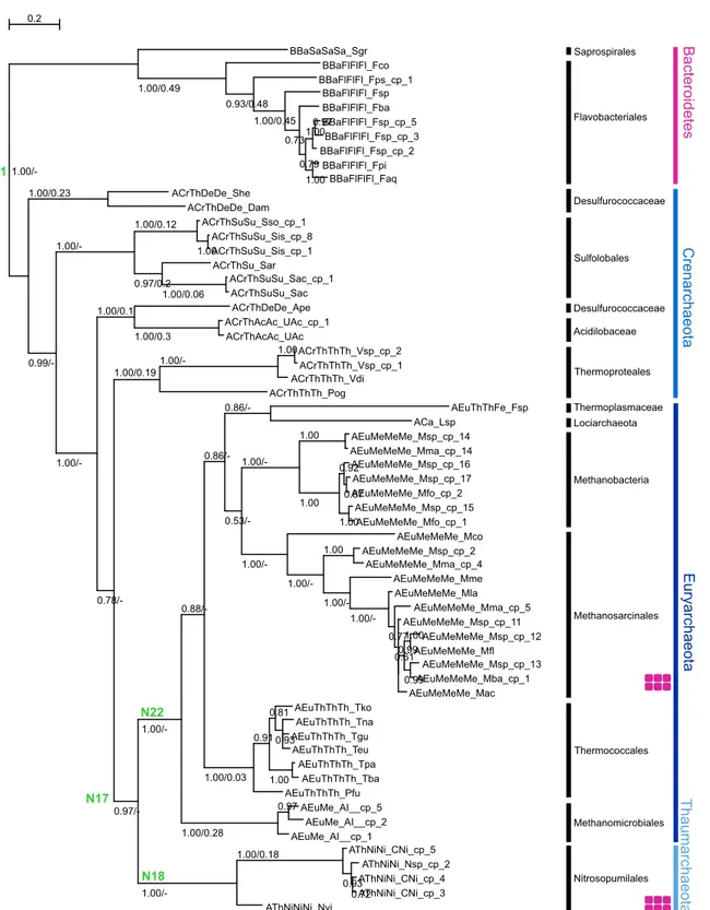
3.3 Phylogeny of the manually curated sequence set used for ASR of GGGPS prede- cessors . . . . 29

3.4 The phylogeny of the sequence set generated by means of FitSS4ASR for ASR of GGGPS predecessors . . . . 30

4.1 Reactions catalyzed by the α-subunit (α-reaction), the β-subunit (β-reaction), and the TS complex (αβ-reaction). . . . 38

4.2 Assembly of LBCA α- and β-subunits to the TS complex. . . . 41

4.3 Crystal structure of the LBCA TS complex . . . . 42

4.4 Comparison of H-bonds between LBCA TS and stTS. . . . 43

4.5 Phylogenetic tree for the reconstruction of LBCA TS . . . . 49

4.6 Amino acid sequences of LBCA TS subunits . . . . 50

4.7 Thermal stability of LBCA α- and β-subunits . . . . 50

4.8 Reaction course of two different nucleophiles at the LBCA β-subunit active site . 51 4.9 Hydrogen bond network at the α/β interfaces of LBCA TS and stTS . . . . 52

5.1 Structure and reaction of the ImGP synthase (HisF:HisH complex) . . . . 58

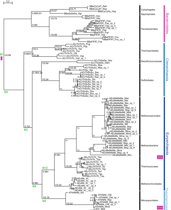
5.2 Phylogenetic tree based on 87 concatenated HisF and HisH sequences from seven phylogenetic clades . . . . 63

5.3 Model of the LUCA-HisF:zmHisH complex . . . . 65

5.4 Stepwise identification of a HisF hotspot for binding to zmHisH . . . . 66

5.5 Identification of interface residues determining the affinity of LUCA-HisF and

Anc1pa-HisF for zmHisH by means of in silico design . . . . 66

(16)

5.6 Fluorescence titration experiments to determine dissociation constants for the interaction of zmHisH with various HisF subunits . . . . 70 5.7 Far-UV circular dichroism spectra of HisF proteins used for fluorescence titration

with zmHisH . . . . 71 5.8 Phylogenetic tree used for reconstruction of ancestral HisF sequences after opti-

mization with FastML . . . . 72

(17)

List of Tables

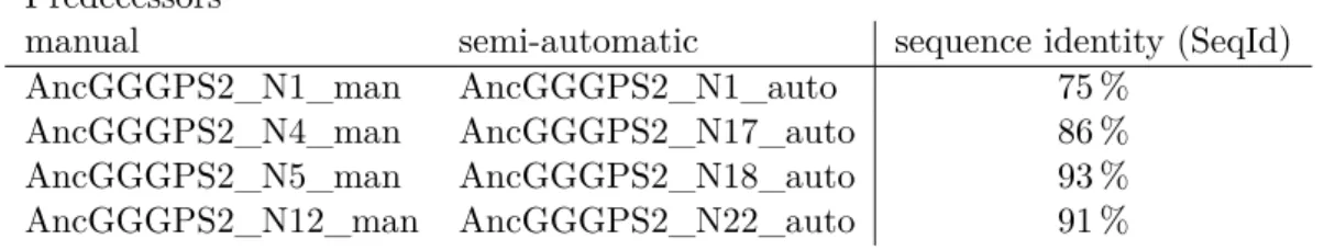
3.1 Comparing predecessors from manual and semi-automatic approach by their SeqId 31 3.2 MSA consisting of the 87 sequences of GGGPS2_man and reconstructed prede-

cessors . . . . 36 3.3 MSA consisting of the 61 sequences of GGGPS2_auto and reconstructed prede-

cessors . . . . 36 3.4 Phylogenetic tree deduced for GGGPS2_man . . . . 36 3.5 Phylogenetic tree deduced for GGGPS2_auto . . . . 36 4.1 Steady-state enzymatic parameters for the α-reaction of LBCA TS and ecTS . . 43 4.2 Steady-state enzymatic parameters for the β-reaction of LBCA TS and ecTS . . 44 4.4 Crystal structure of the LBCA TS: Data collection and refinement . . . . 53 4.5 Multiple sequence alignment of concatenated α- and β-subunits of modern TS

and sequences of LBCA α- and β-subunits . . . . 53 5.1 Dissociation constants for the interaction of zmHisH with various HisF proteins . 64 5.2 Nucleotide and amino acid sequences for Anc1pa-HisF, Anc1pa-HisF*, Anc1tm-

HisF, and Anc2tm-HisF . . . . 73 5.3 Aligned sequences of modern HisF proteins used for phylogenetic analysis and of

LUCA-HisF . . . . 73 5.4 Log likelihood values and posterior probabilities of the reconstructed ancestral

sequences at each position . . . . 73

5.5 Hotspot prediction for HisF residues in ImGPS interfaces . . . . 73

(18)

(19)

Chapter 1 General Introduction

1.1 Evolution in Biology

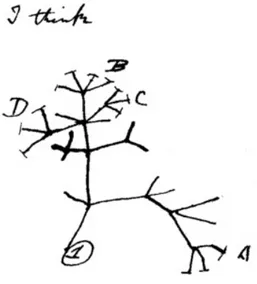
Since Darwin has postulated his theory of evolution (Darwin, 1859), it is generally accepted that today’s living species evolved from a common origin. The diversity of life has been generated by millions of generations driven by natural selection. The idea of a common ancestor (CA) and the diversity of today’s living species are best explained by a branching pattern of evolution, called an evolutionary tree. This concept is based on the principle of homology, which was defined by Darwin as the shared ancestry within a pair of structures (e. g. bones), or genes. Studying homologous structures from different animals in detail, Darwin could deduce a trend of adapta- tion to a specific habitat or function. Thus, Darwin was able to derive a first evolutionary tree (Figure 1.1) and since then a more and more sophisticated theory of evolution was developed that stimulated many fields of life science, e. g. the field of phylogenetic systematics (Hennig, 1965).

Figure 1.1: Darwin’s sketch of the tree of life. A drawing from Darwin’s notebook showing his

first sketch of an evolutionary tree from around 1837. Adapted from Darwin (1837).

(20)

Rhodopirellula baltica

Borrelia burgdorferi

Treponema denticola Treponema pallidum

Leptospira interrogans 56601

Campylobacter jejuni

Helicobacter pylori 26695 Pseudomonas aeruginosa

Ralstonia solanacearum Pseudomonas syringae

Xanthomonas campestris

Bradyrhizobium japonicum Rhizobium loti

Rhizobium meliloti Neisseria meningitidis B Bordetella bronchiseptica

Bordetella parapertussisBordetella pertussis

Chromobacterium violaceum Escherichia coli K12

Salmonella typhi

Salmonella typhimurium Shigella ﬂexneri 2a 301

Yersinia pestis CO92

Vibrio cholerae Vibrio parahaemolyticus Vibrio vulniﬁcus CMCP6 Haemophilus inﬂuenzae

Haemophilus ducreyi Pasteurella multocida

Coxiella burnetii

Rickettsia conorii Rickettsia prowazekii

Chlamydia trachomatis Bacteroides thetaiotaomicron Porphyromonas gingivalis

Wolinella succinogenes Desulfovibrio vulgaris Nitrosomonas europaea

Bdellovibrio bacteriovorus

Rhodopseudomonas palustris

Chlorobium tepidum

Synechocystis sp. PCC6803 Prochlorococcus marinus SS120

Staphylococcus epidermidis

Deinococcus radiodurans

Streptococcus mutans Streptococcus pneumoniae TIGR4

Streptococcus pyogenes M1 Enterococcus faecalis

Lactococcus lactis Bacillus subtilis Clostridium acetobutylicum

Clostridium perfringens Clostridium tetani

Lactobacillus plantarum Listeria monocytogenes EGD Listeria innocua

Corynebacterium diphtheriae

Corynebacterium glutamicum

Mycobacterium bovis Mycobacterium leprae

Mycobacterium paratuberculosis Streptomyces coelicolor Mycoplasma gallisepticum

Mycoplasma genitalium Mycoplasma pneumoniae Mycoplasma pulmonis Methanococcus jannaschii

Methanosarcina mazei Methanosarcina acetivorans

Archaeoglobus fulgidus Pyrococcus furiosus

Sulfolobus solfataricus Thermoplasma acidophilum

Methanopyrus kandleri

Thermotoga maritima Xylella fastidiosa 9a5c

Arabidopsis thaliana

Oryza sativa

Schizosaccharomyces pombe Saccharomyces cerevisiae

Leishmania major

Caenorhabditis briggsae Caenorhabditis elegans

Drosophila melanogaster Danio rerioGallus gallus

Pan troglodytes Homo sapiens Mus musculus Rattus norvegicus

Pyrobaculum aerophilum

Mycoplasma penetrans Pyrococcus abyssi

Brucella melitensisBrucella suis

Takifugu rubripes

Helicobacter hepaticus

Synechococcus elongatus Gloeobacter violaceus Eremothecium gossypii

Streptomyces avermitilis Lactobacillus johnsonii

Geobacter sulfurreducens Plasmodium falciparum

Wigglesworthia brevipalpis

Methanococcus maripaludis

Mycoplasma mycoides

Leptospira interrogans L1-130 Dictyostelium discoideum

Cyanidioschyzon merolae

Thermoplasma volcanium Pyrococcus horikoshii

Aeropyrum pernix

Fibrobacter succinogenes

Prochlorococcus marinus CCMP1378 Aquifex aeolicus Halobacterium sp. NRC-1

Neisseria meningitidis A

Wolbachia sp. wMel Shewanella oneidensis

Photobacterium profundum

Prochlorococcus marinus MIT9313

Fusobacterium nucleatum Mycobacterium tuberculosis CDC1551 Mycobacterium tuberculosis H37Rv Escherichia coli O157:H7

Chlamydophila caviae Chlamydia muridarum

Synechococcus sp. WH8102

Helicobacter pylori J99

Bacillus halodurans

Xanthomonas axonopodis Buchnera aphidicola Sg

Phytoplasma Onion yellows

Nostoc sp. PCC 7120 Sulfolobus tokodaii

Chlamydia pneumoniae AR39 Chlamydia pneumoniae CWL029 Buchnera aphidicola

APS

Thermoanaerobacter tengcongensis

Ureaplasma parvum

Buchnera aphidicola Bp

Chlamydia pneumoniae J138 Photorhabdus luminescens

Corynebacterium eﬃciens Escherichia coli EDL933

Caulobacter crescentus

Staphylococcus aureus Mu50 Staphylococcus aureus N315

Nanoarchaeum equitans

Pseudomonas putida

Streptococcus pneumoniae R6

Anopheles gambiae

Agrobacterium tumefaciens WashU Agrobacterium tumefaciens Cereon

Chlamydophila pneumoniae TW183 Oceanobacillus iheyensis

Xylella fastidiosa 700964

Giardia lamblia

Streptococcus pyogenes MGAS8232

Yersinia pestis KIM

Methanobacterium thermautotrophicum

Streptococcus pyogenes SSI-1

Vibrio vulniﬁcus YJ016

Staphylococcus aureus MW2

Corynebacterium glutamicum 13032 Bacillus anthracis

Shigella ﬂexneri 2a 2457T

Streptococcus pyogenes MGAS315

Tropheryma whipplei T

wist Blochmannia ﬂoridanus

Salmonella enterica

Gemmata obscuriglobus Streptococcus agalactiae V Streptococcus agalactiae III

Biﬁdobacterium longum Escherichia coli O6

Tropheryma whipplei TW08/27 Bacillus cereus

ATCC 10987 Bacillus cereus

ATCC 14579

Yersinia pestis Medievalis

Solibacter usitatus Cryptosporidium hominis

Acidobacterium capsulatum

Dehalococcoides ethenogenes Thermus thermophilus

Listeria monocytogenes F2365 Mycoplasma mobile

Thalassiosira pseudonana

Colored ranges

Bacteria Eukaryota Archaea

Tree scale: 0.1

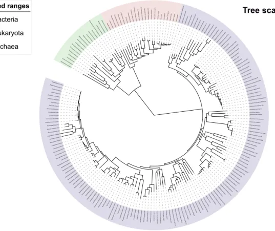
Figure 1.2: The tree of life representing the diversity of all living organisms. This tree is based on a phylogeny resulting from the analysis of 181 sequences. The tree supports the existence of three superkingdoms, namely Bacteria (blue), Eukaryota (red), and Archaea (green). Adapted from iTOL (Letunic and Bork, 2016).

Nowadays, evolution is studied on the molecular level albeit with the same concepts in-

troduced by Darwin. With the advent of deoxyribonucleic acid (DNA) sequencing technology,

genes are compared on their DNA sequences and termed homologous, if sequences share a certain

level of similarity. Analogously, the homology of encoded proteins can be assessed by comparing

the protein sequences (Needleman and Wunsch, 1970). Thus, the comparison of macroscopic

traits like bones was replaced by the analysis of molecular features. Computational biology con-

tributed a lot to evolutionary biology, for example with the development of phylogenetic models

that describe mutational events on the level of DNA or proteins (Felsenstein, 1981). In contrast

to mutations on the macroscopic level, it is uncomplicated to assess all kinds of alterations by

means of probabilistic measures (Dayhoff et al., 1978). With an evolutionary model in hand,

the computation of a phylogenetic tree is straightforward and can be formulated (for example)

as an optimization problem. Thus, by choosing a proper set of genes or proteins, it is nowadays

feasible to deduced a tree of life, which comprises representatives of all major clades that con-

stitute the leaves (Letunic and Bork, 2016); (Figure 1.2). The root of the tree represents the

CA according to Darwin’s theory. The path from the CA represented by the root to present day

organisms (outer circle) has been driven by natural selection and cannot be followed in detail

(21)

1.2 Ancestral Sequence Reconstruction

due to lacking intermediates.

However, in order to verify Darwin’s theory and to understand evolution in detail, the desire to elucidate the appearance of ancestral traits has been immense. Oldest fossils date back to 635 million years ago (Gehling et al., 2000), thus the appearance of several animals like mam- mals or traits like feathers could be reconstructed. Unfortunately, microfossils that date back to 4.1 billion years ago (Bell et al., 2015) do not allow for the reconstruction of fragile organelles or individual macromolecules. On the other hand, Pauling and Zuckerkandl (1963) realized already in 1963 that molecules bear a signal of their history. After reliable algorithms had been designed (Felsenstein, 1981), an alternative to the analysis of fossils opened up, which is the reconstruc- tion by means of phylogenetic methods. Nowadays, tremendous computer power is at hand and highly sophisticated sampling methods like Markov Chain Monte Carlo (MCMC) algorithms are used for Bayesian inference or maximum likelihood (ML) approaches. Thus, algorithms based on phylogenetic models are a common means for the computation of phylogenetic trees, which are subsequently used to reconstruct the sequences of extinct predecessors. Having these sequences at hand, a straightforward protocol makes it possible to express the proteins and to characterize them by means of all the experimental techniques of biochemistry and biophysics. Thus, this combination of computational and experimental biology has already been widely used (Liberles, 2007) to either test hypothesis of adaption (Frumhoff and Reeve, 1994), reconsider evolutionary relationships between the three superkingdoms (Gupta, 1998) or determine the origin of eukary- otes cell (López-García and Moreira, 2015; Eme et al., 2017). The fundamental results made it possible to understand adaptations, e. g. on climate conditions (Hoffmann and Sgrò, 2011) or interaction diversification (Plach et al., 2017) during evolution.

1.2 Ancestral Sequence Reconstruction

Since the 1980ies, novel computational methods allow the reconstruction of ancestral sequences and to travel back in time (Thornton, 2004; Hanson-Smith et al., 2010). This in silico technique, termed ancestral sequence reconstruction (ASR), requires four steps (Merkl and Sterner, 2016), which are depicted in (Figure 1.3 A - G).

Commonly, homologous sequences are retrieved from databases like UniProtKB (Apweiler

et al., 2004) or with the help of BLAST (Altschul et al., 1990) to compile a set of extant sequences

(Figure 1.3 A). The number of extant sequences required for an ASR depends on the protein-

specific mutation rates and the time span of interest. Thus, between 11 (Yokoyama et al., 2008)

and up to 200 or more sequences (Perez-Jimenez et al., 2011; Harms et al., 2013) were used

for ASR. These extant sequences are then used to create a multiple sequence alignment (MSA)

(Figure 1.3 A). During recent years, several algorithms showing comparable alignment quality

have been introduced and were used to map residues to protein positions. Based on an MSA, a

phylogenetic tree is deduced by means of state of the art methods like ML or with a Bayesian

(22)

A

_Anc1

Anc2 Anc3

Anc4 Anc5

Anc6

Anc7 Anc9 Anc8 Seq1

Seq10

...

Anc1

Anc9

...

B C D

F E G

M L A K R I I A C L N V K - - D G R V V M L A K R I I P C L D V K - - D G R V V F G S Q A V V V A I D A K R V D G E F M H M A L R I I P C L D I D G G A K V V V M L A K R I I A C L D V K - - D G R V V - MG K I V L I V D D A T - - N G R - - - - MQ R V V V A I D A K R V D G E F M - - MQ R V V V A I D A K R V D G E F M - - MQ R V V V A I V A K R V D G E F M M L A K R I I A C L D V K - - D G R V V

M L A K R I I A C L N V K D G R V V K G - - - - R I I S C MD V K N N Y V V K G M L - - R I I S C L D I K N N F V V K G - - - - R I I S C F D V K N N M V V K G M L K K R I I P V Q L L L N N R L V K T M L A K R I I A C L D I K D G Y V V K G M L K T R I V G V L V V K G G I V V Q S M L A K R I I A C L D V H N G V V V K G M L A K R I I P C L D V A N N K V I K G

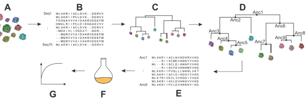
Figure 1.3: “Resurrection” of ancestral proteins based on ASR. The procedure consists of the steps illustrated in panels A - G. A set of homologous proteins (A) is chosen as the starting point.

The protein sequences are aligned to an MSA (B) and a phylogenetic tree is derived (C). By means of the phylogenetic tree, the sequence set, and a substitution model, the ancestral sequences related to the bifurcations of the tree are inferred (D, E). Based on these sequences, proteins can be produced recombinantly, (F) and characterized by means of biophysical and biochemical methods (G).

approach. There are several programs available, like the ML approach RAxML (Stamatakis, 2014) or the Bayesian approach MrBayes (Holder and Lewis, 2003). To select the best fitting model for the data set at hand, ProtTest (Abascal et al., 2005) can be used to identify the best generating evolutionary model. The validity of the derived phylogenetic model can be confirmed with bootstrapping in an ML analysis (Felsenstein, 1985) or with the help of multiple samples from the posterior distribution for Bayesian analyses (Rannala and Yang, 1996). The chosen extant sequences and the derived phylogenetic tree (Figure 1.3 A, C) combined with a substitution model form the basis for the computation of the ancestral sequences. In principle, ASR computes for each internal node a matrix indicating for each residue position the probability distribution of all amino acids. For the sake of simplicity, in most experiments the sequence with the highest likelihood has been considered for each internal node (Figure 1.3 D, E); see for example (Perica et al., 2014). Several programs, compared by Joy et al. (2016), are available for inferring ancestral sequences. An experimental characterization of the corresponding proteins requires the production of the protein in a recombinant form, expression of the protein in host cells and the characterization with biochemical experiments, e. g., activity assays (Figure 1.3 E - F).

Driven to extremes, ASR makes it possible to characterize ancestral proteins that date

back to the Last Universal Common Ancestor (LUCA) that existed in the Paleoarchean era,

i. e. at least 3.5 billion years ago (Nisbet and Sleep, 2001). These “resurrection” experiments

have elucidated many aspects of the early life on Earth and the evolution of proteins and macro-

molecular complexes. For example, Wheeler et al. (2016) discussed several ancestral proteins,

e. g. the ancestor of thioredoxin (Perez-Jimenez et al., 2011), which exhibit elevated thermosta-

bility. Busch et al. (2016) characterized an ancestral enzyme complex, namely the tryptophan

synthase (TS). Regarding to functional properties at early stages of evolution, several ancestral

(23)

1.2 Ancestral Sequence Reconstruction

proteins exhibit broad substrate recognition, like the ancestor of the serine protease (Wouters et al., 2003).

A second reason for the great success is that ASR adds a further dimension to sequence analysis: From an evolutionary point of view, extant homologs represent variants observed for one point in time, thus the comparison of these proteins was termed “horizontal” approach. In contrast, ASR is a “vertical approach”, as it takes into account the evolutionary history of the proteins under study. Considering the chronology of mutations is more straightforward to iden- tify crucial but subtle amino acid differences (Harms and Thornton, 2010), because the sequences generated for internal nodes are similar to each other and contain fewer neutral mutations than many extant sequences. Thus, vertical approaches can drastically reduce experimental efforts to identify key residues.

For example, the vertical approach has been used to elucidate the linkage between protein structure and its function (Gumulya and Gillam, 2017). Additionally, Perica et al. (2014) showed that ancestral pyrimidine operon regulatory protein, PyrR, exhibit different oligomeric states and revealed 11 key mutations controlling this state. Ugalde et al. (2004) examined green flourescent protein (GFP)-like proteins from corals, where the ancestral genes illuminate in green, which turned to a red emission in the extant corals through a stepwise adaption. Moreover, ancestors of the sugar isomerase HisA from the histidine biosynthesis were examined to reveal the positions leading to promiscuity, i. e. a broad protein specificity (Plach et al., 2016).

Interestingly, it turned out that resurrected proteins are generally more stable and possess often a broader substrate specificity than the extant sequences used for reconstruction (Wheeler et al., 2016). It is a matter of debate, whether this higher thermostability is an artifact of the ASR protocol or a general feature of ancestral proteins (Williams et al., 2006). Protein design problems can profit from these properties as shown for the design of 3-isopropylmalate dehydro- genase (Watanabe et al., 2006) leading to designed enzymes with even higher thermostability.

Zakas et al. (2017) designed a pharmaceutical important coagulation factor VIII that benefited from ASR with respect to biosynthetic efficiency, specific activity, stability, and immune reac- tivity. Cole et al. (2013) introduced a method that exploits a vertical approach as an additional source of information for altering or enhancing the function of the protein in protein engineering.

The application of ASR profited from the rapid progress of quite different life-science

technologies: The outcome of sequencing projects led to an exponential growth of databases

making a huge number of proteins available for ASR. Progress in gene-synthesis accompanied by

a drastic reduction of costs turned resurrection experiments into a cost-effective tool to generate

results in a timely manner. Ironically, the step to be expected least critical in resurrection

experiments, namely ASR, became a bottleneck. As illustrated above, ASR can be divided into

four steps, and some critical aspects will be highlighted in the following. The final outcome of

ASR are the sequences of the internal nodes, whose composition depends on the phylogenetic

tree computed beforehand for the chosen set of extant sequences and by applying an evolutionary

(24)

A

M L A K R I I A C L N V K - - D G R V V M L A K R I I P C L D V K - - D G R V V F G S Q A V V V A I D A K R V D G E F M H M A L R I I P C L D I D G G A K V V V M L A K R I I A C L D V K - - D G R V V - MG K I V L I V D D A T - - N G R - - - - MQ R V V V A I D A K R V D G E F M - - MQ R V V V A I D A K R V D G E F M - - MQ R V V V A I V A K R V D G E F M M L A K R I I A C L D V K - - D G R V V Seq10

...

Seq1

B

topology branch

length

C

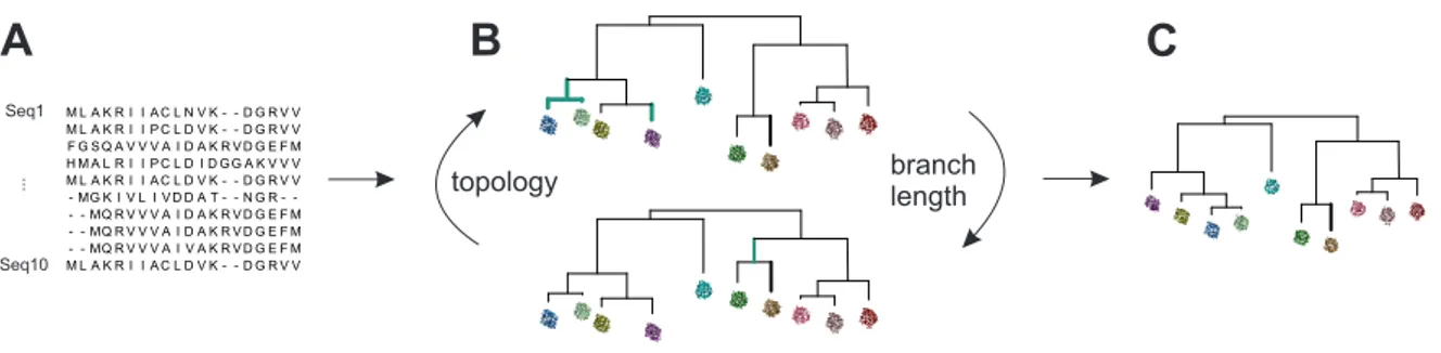
Figure 1.4: Calculation of a phylogenetic tree. The procedure consist of the steps illustrated in A - C. Based on an MSA consisting of extant sequences (A) a first phylogenetic tree is derived (B). The topology and the branch lengths are consecutively optimized (changes are indicated in cyan) in order to increase the likelihood of the phylogenetic tree. These issues are solved as part of an optimization problem to obtain the final tree (C), which is the most likely tree with respect to the input sequence set and the chosen phylogenetic model.

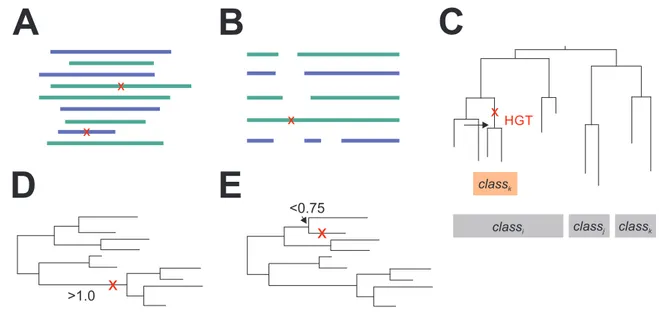
model. However, the user has to assess critically the phylogenetic tree prior to the reconstruction step in order to exclude errors that might rule out a valid reconstruction. Most critical are the length of all branches and the topology of the tree (Merkl and Sterner, 2016). For a reliable reconstruction, all branch lengths must be lower than one mutation per site to allow for a modelling of all mutations. The topology should be as unambiguous as possible to rule out alternative evolutionary scenarios. Even, if all sequences share a CA, i. e. are homologous, hor- izontal gene transfer (HGT) may cause topologies that are not compatible with the expected phylogeny. If the proteins under study are multi domain proteins, their composition has to be compared with great care to ensure that all proteins possess the same domains in the same order.

A further problem that can impede reconstruction is the number of insertions and deletions that occurred during the genesis of the recent sequences. Only few algorithms can model some of these events in an evolutionary correct manner (Löytynoja and Goldman, 2008; Ashkenazy et al., 2012). Taken together, these constraints emphasize the judicious selection of the sequence set.

This choice implies a sequence selection; however, their suitability for ASR is only confirmed after the computation of a tree. It follows that sequence selection is an iterative process, which requires to integrate a phylogenetic analysis.

It is the calculation of a phylogenetic tree (Figure 1.4) that turns ASR into a time-

consuming process. As indicated above, the phylogenetic tree is derived from a given MSA of

extant sequences (Figure 1.4 A). The calculation of the phylogenetic tree (Figure 1.4 B) can

be viewed as an optimization problem: Topology and branch lengths are optimized consecu-

tively (Figure 1.4 C, indicated in cyan) in order to increase the likelihood of the tree. After

several rounds of optimization, the most likely phylogenetic tree regarding to the sequence data

is obtained (Figure 1.4 D) and then the suitability of the tree for ASR can be assessed. Phy-

logenetic trees not suitable for ASR cannot be changed directly, as the appearance of the tree is

determined by the sequence set. Thus, the sequence set has to be changed in order to support a

tree suitable for ASR (Merkl and Sterner, 2016). However, alterations in the sequence set often

(25)

1.3 Aim and Scope of this Work

lead to unexpected changes in the topology, thus several rounds of alterations in the sequence set are necessary to obtain a suitable tree for ASR.

Since popularity and strength of ASR has increased during the last years, not only com- mand line tools, but also simple-to-use webserver or programs are available that deduce a phy- logenetic tree (Guindon et al., 2010; Stamatakis, 2014; Lartillot et al., 2009; Ronquist and Huelsenbeck, 2003). If a suitable data set is at hand, protocols that execute all steps of ASR can be applied (Tamura et al., 2011; Hanson-Smith and Johnson, 2016; Dereeper et al., 2008).

However, a protocol for the compilation of a suitable sequence set leading to a reliable tree is not available. Moreover, all programs can only handle a relatively small number of sequences, which implies their deliberate selection from the enormous number of sequences deposited in databases like InterPro or UniProt (Li et al., 2008; Frickey and Lupas, 2004). Due to the design of the algorithms, between 150 and 200 sequences should be chosen for an ML approach and 30 to 80 present the limit for a Bayesian approach (Hanson-Smith and Johnson, 2016; Dereeper et al., 2008). So far, there exists no broadly applicable protocol for sequence selection; it is common practice to pick them manually with the help of an intuitive presentation (Hanson-Smith and Johnson, 2016; Dereeper et al., 2008). A few algorithms have been established to take over at least some part of the filtering procedure. Starting with sequences collected by means of a BLAST search, the algorithm implemented by Goremykin et al. (2010) excludes sequences based on their similarity and outputs sets of maximal 150 entries; a similar approach is cd-hit (Li and Godzik, 2006). Other programs, like Gblocks (Castresana, 2000) or trimAl (Capella-Gutiérrez et al., 2009) eliminate rows from the MSA that contain a large number of gaps in order to increase the quality of the phylogenetic signal. Thus, methods are available that solve some subtasks of sequence preparation; however, there exists no protocol that considers the above-mentioned criteria in a comprehensive manner.

1.3 Aim and Scope of this Work

During the last years, ASR turned from a method mastered by few specialists to a frequently used technology, although a generally accepted protocol is missing. In order to allow for the reliable reconstruction of proteins, a standard protocol was established within the scope of this thesis.

It was used to reconstruct ancestors of the imidazole glycerol phosphate synthase (ImGPS) and

the TS that were both characterized on their biochemically properties. Within the protocol,

several features were used for sequence filtering, namely the length of the unaligned sequences,

the amount of indels in the alignment, the length of the branches and the value of bootstrap

values or posterior probabilities. In addition to this standard protocol a further protocol was

developed to identify crucial positions with the help of a vertical approach, e. g. of complex

formation. A combination of biochemical characterization and the in silico assessment of these

proteins allowed us to narrow down several candidate positions to one crucial positions. Due to

(26)

the versatility of vertical approaches, the protocol can be adapted to different scientific problems.

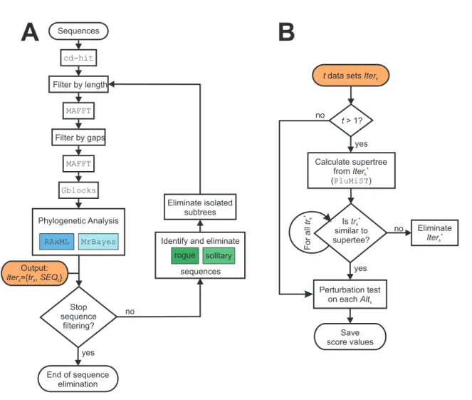
Based on the standardized protocol, sequence selection was further improved by focusing on their rational selection in an automated manner. To perform this task, FitSS4ASR was devel- oped that uses iteratively the above-defined features to evaluate sequence sets and phylogenetic trees and to remove sequences. The outcome are several alternative sets and the user can choose the most appropriate one. To support the user’s decision, FitSS4ASR computes several scores assessing the phylogenetic variety of the sequence set and the robustness of the tree. Thus, FitSS4ASR makes it possible to find a suitable data set in a semi-automated manner.

As already mentioned, a standard protocol for ASR was established within the reconstruc- tion of ancestors of ImGPS and TS. In order to reveal the level of specialization of an ancestral enzyme complex, the TS from the last bacterial common ancestor (LBCA) was reconstructed and experimentally characterized. It turned out that the reconstructed TS consists of two TrpA and two TrpB subunits as the TS from Salmonella typhimurium (stTS). Moreover, a comparison of the ancestral protein and the extant proteins made clear that TrpA and TrpB activate each other allosterically. A biochemical characterization showed a deactivation in the ancestral com- plex, whereas an activation occurs in the extant complex. Comparisons of the crystal structures of both complexes were conducted to link the differences in the activation process to differences on substructure or residue level; however, we were not able to pinpoint residues or structural parts responsible for the allosteric activation.

A second application of ASR has been performed on ImGPS, which consists of the synthase HisF and glutaminase HisH. To identify hotspots of complex formation, reconstructed HisF sub- units were combined with the HisH subunit from Zymomonas mobilis (zmHisH). Interestingly, two ancestral HisF subunits had a differing binding behavior; thus, mutational experiments combined with in silico predictions were sufficient to narrow down the candidate positions to one hotspot. This application is an example indicating how a vertical approach allows for a specific property the rapid identification of a crucial position.

1.4 Guide to the Following Chapters

Each of the following four chapters corresponds to one manuscripts; two of them have been published and one is an accepted chapter of the book “Computational Methods in Protein Evolution”. One chapter contains unpublished data.

The manuscript Ancestral Sequence Reconstruction as a Tool for the Elucidation

of a Stepwise Evolutionary Adaptation describes our standard protocol of ASR and sev-

eral pitfalls. Taking ImGPS as an example, it is also shown, how ASR can be used to identify

hotspots in protein-protein interactions. ImGPS is a heterodimer consisting of the synthase

subunit HisF and the glutaminase subunit HisH. By comparing the sequences of intermedi-

ate sequences leading from the LUCA-HisF to the extant HisF from Pyrobaculum arsenaticum

(27)

1.4 Guide to the Following Chapters

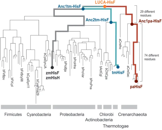
(paHisF) a neighbored pair of ancestral HisF subunits differing in the strength of complex formation to the extant zmHisH was identified. The candidate positions responsible for the different binding behavior are assessed by comparing the sequences. Furthermore, the approach is illustrated to narrow down few candidate positions with the help of structural and biochem- ical evaluation in combination with in silico predictions: Specifically, for the ancestral HisF subunits, it was demonstrated that one hotspot modulates protein-protein interaction. The in silico prediction was confirmed by an assessment of the complex consisting of HisF from Ther- motoga maritima (tmHisF) and zmHisH. Furthermore, the transferability of the protocol to other scientific problems is shown.

The following chapter Sequence Selection by FitSS4ASR Alleviates Ancestral Se- quence Reconstruction as Exemplified for Geranylgeranylglyceryl Phosphate Syn- thase contains unpublished data and describes the novel protocol FitSS4ASR that supports the user in selecting sequences for ASR (see also chapter 2). FitSS4ASR requires as input a sequence set that consist of several thousand homologs. This set is iteratively reduced with the help of sequence filters and by analyzing phylogenetic trees. The output of FitSS4ASR are several sequence sets of differing size, which are scored with respect to their suitability for ASR.

The suitability of FitSS4ASR was made plausible by analyzing the trees deduced for the geranyl- geranylglycerol phosphate synthase (GGGPS), which is an enzyme that forms taxon-specifically homodimers or homohexamers. The computed trees and inferred ancestors were compared to show the validity of FitSS4ASR.

The publication The Ancient Nature of Allostery and Substrate Channeling in the Tryptophan Synthase Complex reports on an application of ASR related to the TS from the LBCA. TS consists of the subunits TrpA and TrpB and the reconstructed sequences were the basis for a recombinant production and the subsequent experimental characterization.

It turned out that the sophisticated allosteric activation observed between the two subunits of TS from Salmonella typhimurium existed already at an early phase of evolution. Comparison of crystal structures made clear that the structure of the subunits and their arrangement in the complex were not altered within 3.14 billion years.

The publication Combining Ancestral Sequence Reconstruction with Protein De-

sign to Identify an Interface Hotspot in a Key Metabolic Enzyme Complex describes

an application of a vertical approach used to identify binding hotspots of the protein-protein in-

terface in ImGPS. The binding strength of reconstructed HisF enzymes to the zmHisH subunit

was experimentally determined. Correlating these data with differences in the reconstructed

interfaces, putative hotspots were predicted, which were further assessed by means of other in

silico methods. We could show that one residue position is crucial for binding.

(28)

(29)

Chapter 2 Ancestral Sequence Reconstruction as a Tool for the Elucidation of a Stepwise Evolutionary Adaptation

Kristina Straub and Rainer Merkl

To appear as a book chapter of

Computational Methods in Protein Evolution: Methods and Protocols, Springer, New York. In Press, Editor: Tobias Sikosek

Key words ancestral sequence reconstruction, vertical analysis, evolutionary biochemistry, in silico mutagenesis, protein-protein interaction.

Abstract