Multi-objective optimization for an automated and simultaneous phase and baseline correction of NMR spectral data.

Multi-objective optimization for an automated and simultaneous phase and baseline correction of NMR spectral data.

Mathias Sawall^a, Erik von Harbou^b, Annekathrin Moog^a, Richard Behrens^b, Henning Schr¨oder^a, Jo¨el Simoneau^d, Ellen Steimers^b, Klaus Neymeyr^a,c

aUniversit¨at Rostock, Institut f¨ur Mathematik, Ulmenstraße 69, 18057 Rostock, Germany

bTechnische Universit¨at Kaiserslautern, Lehrstuhl f¨ur Thermodynamik, Erwin-Schr ¨odinger-Straße 44, 67663 Kaiserslautern, Germany

cLeibniz-Institut f¨ur Katalyse e.V. an der Universit¨at Rostock, Albert-Einstein-Straße 29a, 18059 Rostock

dUniversit´e de Sherbrooke, Department of Chemical&Biotechnological Engineering, 2500 Blvd. de L’Universit´e, Sherbrooke, Canada

Abstract

Spectral data preprocessing is an integral and sometimes inevitable part of chemometric analyses. For Nuclear Mag- netic Resonance (NMR) spectra a possible first preprocessing step is a phase correction which is applied to the Fourier transformed free induction decay (FID) signal. This preprocessing step can be followed by a separate baseline cor- rection step. Especially if series of high-resolution spectra are considered, then automated and computationally fast preprocessing routines are desirable.

A new method is suggested that applies the phase and the baseline corrections simultaneously in an automated form without manual input, which distinguishes this work from other approaches. The underlying multi-objective op- timization or Pareto optimization provides improved results compared to consecutively applied correction steps. The optimization process uses an objective function which applies strong penalty constraints and weaker regularization conditions. The new method includes an approach for the detection of zero baseline regions. The baseline correction uses a modified Whittaker smoother. The functionality of the new method is demonstrated for experimental NMR spectra. The results are verified against gravimetric data. The method is compared to alternative preprocessing tools.

Additionally, the simultaneous correction method is compared to a consecutive application of the two correction steps.

Key words: NMR data preprocessing, automated phase correction, automated baseline correction, multi-objective minimization, Whittaker smoother.

1. Introduction

NMR spectroscopy is of extraordinary importance for many research fields in science and medicine. The Nobel lectures of Richard R. Ernst (1991), K. W¨uthrich (2002) and P.C. Lauterbur and P. Mansfield (2003) provide an excellent overview on the development of NMR spectroscopy and its significance for various fields of application [10, 27, 17].

This paper focuses on NMR spectroscopy in chemistry or chemical engineering and the problem that NMR spectra often suffer from various types of misadjustment, distortions and noise. The zero-order misadjustment refers to the phase difference of the reference phase and the phase which is used by the FID signal recording detector [4]. The first-order misadjustment can be caused by different sources, e.g., by the delay between excitation and detection or by phase shifts induced by noise-reducing filters [6]. NMR spectra also suffer from baseline distortions which can be caused for example by the nonlinearity of the filter-phase response, instrumental instabilities, background signals or the discrete nature of the Fourier transformation, see [12]. An efficient and reliable correction of the zero- and first- order misadjustments (phase correction) and a correction of the baseline are prerequisites to facilitate the acquisition of quantitative results from the NMR spectrum [18]. Especially the application of NMR spectroscopy for reaction and process monitoring or process control, which has gained importance over the last years not only due to the development of benchtop NMR spectrometer [16], necessitate automatic and robust correction algorithms that can handle large data sets [3, 19].

In this paper we present a new preprocessing approach for NMR spectral data which allows to correct the zero- and first-order misadjustments in a simultaneous way together with the baseline by means of a multi-objective opti- mization. The simultaneous optimization is a characteristic trait of this new approach.

1.1. Organization of the paper

The paper is organized as follows. Sec. 2 introduces the optimization-based preprocessing approach. To this end, an objective function is suggested which includes penalty and regularization terms. Its minimization amounts to a simultaneous phase and baseline correction. In Secs. 3 and 4 we discuss the step-by-step methods for the phase correction and for the baseline correction. The simultaneous correction method is presented in Sec. 5. The new method is tested for experimental NMR spectra in Sec. 6. This results are compared to the outcome of a computation in which the two correction steps are applied in consecutive manner. Finally, the results are compared to other phase correction methods.

1.2. Notation

We use the following notation for the NMR signal functions.

d^ft denotes a complex valued raw NMR spectrum gained by a Fourier transformation of the free induction decay (FID).

d^pha is a complex NMR signal after a phase correction step. However, only its real part is considered as the NMR spectrum.

d^final is a real-valued NMR signal either after step-wise or simultaneous phase and baseline correction.

d stands for a general real-valued NMR signal with or without prior application of correction steps.

2. Optimization-based data preprocessing

The focus of this paper is on a simultaneous and automated correction of the phase and the baseline of NMR spectra. To this end we use a multi-objective optimization which is a common approach for the implementation of competing constraints, see for example [4] where an entropy minimization approach is used for phase corrections of NMR spectra. It is a well-known fact that a multi-objective optimization problem with competing or even conflicting objective functions often has no single solution which optimizes each constraint. In such cases, the objective functions are called conflicting and the solution of the simultaneous optimization (also known as multi-objective optimization or Pareto optimization) represents a trade-offbetween the conflicting constraints.

Here we consider an objective function which is a weighted sum of penalty functions and regularizing conditions.

This approach makes possible a simultaneous optimization. If all but one of the weight factors are set to zero, then the optimization is applied only to a single constraint. The active constraint can be changed and then the optimization can be restarted. The constraint functions either penalize negative entries of the spectra or are used to regularize the resulting spectra, e.g., in the sense of a small integral or the smoothness of the spectra. If d∈Rⁿdenotes a real-valued (discrete) spectrum, then the objective function f∶Rⁿ→Rreads

f(d)=∑³

i=1

γigi(d/∥d∥^max). (1)

Therein theγi≥0 for i=1,2,3 are real weight factors and∥d∥max=maxi=1,...,n∣di∣is the maximum norm. The three functions g_iare

g1(d)=∑ⁿ

j=1

(min(0,dj+ε1))², g2(d)=∑ⁿ

j=1

(max(0,∣dj∣ −ε2))², g3(d)=ⁿ

−1

∑

j=2

(dj−1−2dj+dj+1)².

For the function g₁we use a relative large weight factorγ₁so that g₁can be considered as a penalty function. For the functions g₂and g₃we take smaller weight factors which results in a regularizing effect in the optimization process.

The function g₁is applied in order to enforce nonnegative results in the optimization process. The constraint function g1 is constructed in a way that only negative portions of d which are smaller than −ε1 are square-summed up and are used for penalization. In other words, small negative entries whose absolute values are smaller thanε1 are not

2

penalized. The function g2is used in order to find a solution with a small integral (case of sharp and isolated peaks).

More precisely, the function g2accesses the discrete integral in terms of sums of squares. In a similar way to g1all entries of∣d∣which are smaller thanε₂do not contribute to this constraint. Thusε₂can be considered as a level of accepted deviation of the baseline from the ideal zero-baseline. Finally, the function g₃sums up the squares of discrete second derivatives of the data. In this way non-smooth solutions are penalized and smooth solutions are favored in the usual way of Tikhonov regularizations. The relationsγ1≫γ2, γ3for the weight factors guarantee that nonnegativity is a stronger constraint (penalization) whereas a small integral and smoothness of the solutions are weaker constraints (regularizations). For the case of weakly perturbed spectra and if sharp peaks (small integral with low smoothness) are desired, then we useγ1=10,γ2=10⁻²andγ3=0 as typical values for the weight constants. Ifγ3is increased, e.g.γ3 =0.1 together withγ1 =10,γ2 =10⁻², then somewhat wider peaks with a slightly increased smoothness are favored.

The control parameterε1 ≥0 in the penalty function g1 is used in order to weaken the nonnegativity constraint in a way that only negative components which are smaller than−ε1 contribute to the sum of squares. The control parameterε2 ≥0 in g2 has a similar effect. Only components of d with∣dj∣≥ε2are taken into consideration for the sum of squares. Thusε2is used to ignore the influence of small entries of the spectrum which are close to zero and which potentially can be traced back to noise or other perturbations. However, evenε1=ε2=0 leads in many cases to useful results. In (1) the functions g_iare applied to normalized spectra d/∥d∥max. Henceε1andε2can be defined in a scaling-independent way. Otherwise, the magnitudes of these control parameters must be adapted to the signal intensity of the spectrum d. If the spectrum includes large perturbations or other systematic biases, then additional functions g_ican be added and further control parametersε_ican be introduced in order to control or to remove the influence of these perturbations.

For the numerical minimization of f we use a combination of a genetic optimization algorithm with population sizes of 20 with 20 generations and an adaptive nonlinear least-squares solver, namely the ACM routine NL2SOL [8].

Our computationally fast program code is written in C and FORTRAN. An implementation in MATLAB by using the routinesfminsearch, a gradient-free simplex minimization algorithm, orlsqnonlin, a nonlinear least-squares solver which uses a subspace trust-region method, is also possible. The optimization-based phase correction, see Sec. 3, and the baseline correction, see Sec. 4, result in preprocessed NMR spectra which fulfill to some extent the various constraints depending on the weight factors. The optimization process can implicitly determine further parameters which belong to the optimal solution. Examples are the optimal phase parametersϕ^∗₀andϕ^∗₁which are optimized in the phase correction, see Sec. 3. The correction steps can be applied consecutively, see Secs. 3 and 4, or simultaneously, see Sec. 5.

3. The automated phase correction

This section recapitulates in short form the step of an automated phase correction for the Fourier transformed spectrum. This phase correction is well-understood, see for example [25, 4, 7, 1]. In Sec. 5 this correction procedure is a building block of the new simultaneous correction scheme. The phase correction fixes two misadjustments of zero- and of first-order by solving an optimization problem for the objective function f given in (1).

3.1. Misadjustments and automated phase correction

Let d^ft∈Cⁿbe the Fourier-transformed FID signal. The aim is to correct the misadjustments of zero-order and of first-order [4, 6]. The fundamental relationship of d^ftto the real and imaginary parts of the phase-corrected spectrum d^pha∈Cⁿis d^pha=(d^ft,e^iφ)with the Euclidean product(⋅,⋅)so that the real and imaginary parts are

Re(d^pha_j )=Re(d^ft_j)cos(φj)−Im(d^ft_j)sin(φj),

Im(d^pha_j )=Im(d^ft_j)cos(φj)+Re(d^ft_j)sin(φj) (2) for j=1, . . . ,n, see [25, 1]. The vectorφdepends on the two real-valued adjustment parametersϕ0andϕ1

φ_j=ϕ₀+ϕ₁j−1

n , j=1, . . . ,n. (3)

The optimal phase angleϕ^∗₀ and phase parameterϕ^∗₁ minimize the objective function f by (1) in a way that f(Re(d^pha(ϕ^∗₀, ϕ^∗₁)))= min

ϕ0∈[−π, π), ϕ₁∈[−nπ,nπ)

f(Re(d^pha(ϕ0, ϕ1)))

and result in the phase corrected spectrum.

3.2. Ambiguity of the phase correction angles

Nonnegativity of the real part Re(d^pha)is not a sufficient constraint for getting unique phase correction parameters ϕ0andϕ1. A formal mathematical argument shows that uniqueness cannot be expected: An ideal NMR spectrum is strictly positive since it is a linear combination with nonnegative coefficients of the (strictly positive) Lorentz profiles [15]. Additionally the relations (2) and (3) are continuous mappings. Thus nonnegativity of Re(d^pha)is guaranteed at least in a small neighborhood of any pair(ϕ0, ϕ1)which represents a positive function Re(d^pha). This yields a continuum of feasible solutions. Similar regions of feasible solutions with respect to the nonnegativity constraint are well-known from other fields of chemometrics; see e.g. [13, 23, 14, 24] for the area of feasible solutions in multivariate curve resolution. However, the ambiguity ofϕ0 andϕ1 is often not very large and uniqueness can be enforced if an additional regularization as by g₂ or g₃ is switched on or if for example an entropy regularization is used [4].

4. The automated baseline correction

The automated baseline correction consists of two steps. In the first step, intervals on the chemical shift axis are detected in which the baseline dominates in the sense that the NMR signals by the chemical sample are of minor importance. In a second step a smooth baseline function on the complete chemical shift axis is fitted to the already identified “pure baseline intervals”. The first step is the more difficult one. The correctness of the complete baseline sensitively depends on the correct detection of the pure baseline intervals. In this section we always assume that the NMR spectrum d^phahas already undergone (a more or less successful) phase correction. Moreover, we consider while referring to d^phaonly its real part.

4.1. Detection of pure baseline intervals

In this section we call a chemical shift value (on the abscissa of an NMR spectrum) a pure-baseline value if its associated signal intensity cannot be assigned to characteristic NMR signals of the chemical sample. Neighboring pure baseline values can be aggregated to pure baseline intervals. Before running the baseline detection procedure, a Savitzky-Golay filter [22, 21] is applied to the NMR spectrum d^pha. The Savitzky-Golay filter is well-known to increase the signal-to-noise ratio and to preserve the characteristic form of the signal. The degree of the approximating polynomial isℓand the width of the moving window is 2m1+1. Thus 2m1+1 consecutive components of the vector d^phaare filtered by polynomial approximations with the polynomial degree of at mostℓ. If d^pha∈Rⁿ, then the Savitzky- Golay filter computes for each integer number i=m1+1,m1+2, . . . ,n−m1a polynomial piof degreeℓ(or less) which approximates the points (of the moving window)

(xj,d^pha_j ), j=i−m1, . . . ,i+m1,

in the least-squares sense. The xj are the discrete values on the abscissa. The least-squares approximation pi is evaluated within the moving window and yields the smoothed data ˜d∈Rⁿas

d˜_i=p_i(x_i), j=i−m₁, . . . ,i+m₁,

and ˜di=difor all remaining indices which do not belong to the moving window. For the remaining abscissa values xi

with i≤m1respectively i≥n−m1the points(xj,d^pha_j )with j=1, . . . ,2m1+1 respectively j=n−2m1, . . .n are used for computing pi. The smoothed approximations are given again in the form ˜di=pi(xi).

4

The next step is to detect abscissa values of the smoothed signal ˜d whose signal intensities are close to their local mean values. To this end we compute the quantities

zi= ⁱ

+m2

∑

j=i−m2

⎛

⎝d˜j−

i+m2

∑

j=i−m2

d˜j

⎞

⎠

2

. (4)

which is the sum of the squares of the deviations of ˜djfrom its mean in a window of the width 2m2+1 and where the outer sum runs again through the 2m2+1 indices of the window which is centered at xi. The ziare computed for the indices i=m2+1,m2+2, . . . ,n−m2.

Remark 4.1. Only the components z_iwith i=m₂+1,m₂+2, . . . ,n−m₂are defined. We set z_i=0 for i=1, . . . ,m₂ and i=m₂+1, . . . ,n−m₂in order to work (for convenience) only with n-dimensional vectors. The baseline detection procedure only needs the components zi, i=m2+1, . . . ,n−m2.

Next the indices are determined for which the (nonnegative) components of z are smaller than a given threshold value. By (4) a component of z vanishes if a consecutive series of components of ˜d in a window with the width 2m₂+1 satisfy a linear relation. We assume such a linear behavior to occur in pure baseline intervals. The selection criterion is as follows: With the control parametersαcrit ∈ (0,1)andδcrit > 0 we define the set of indices which belong to baseline values as

Mbl={i∶ zi/zthres≤δcrit}.

Therein zthresis a threshold value which is computed as follows: First the n−2m2real numbers zm2+1, . . . ,zn−m2 are sorted in ascending order. Then we take the⌈αcrit(n−2m₂)⌉th value of this sequence of sorted numbers. Therein⌈⋅⌉ denotes the ceiling function which is the nearest integer to the argument of the ceiling function which is greater than or equal to its argument. In simple words, the set M_blcontains all indices which belong to windows of the index-width 2m2+1 in which the components behave linearly or nearly linearly.

Appropriate control parameters are m1 = 20, m2 = 40, αcrit = 0.95 and δcrit = 1.1 for the case a step-by-step correction of the phase and the baseline. Appropriate values for simultaneous correction steps are m1=20, m2=40, αcrit=0.5 andδcrit=1.1.

4.2. Baseline computation

The requirements for the baseline are as follows: On the one hand the baseline should be a smooth function and on the other hand the baseline should fit the data d^pha for all indices in the set Mbl. For experimental and noisy data these requirements can be somewhat contradictory as d^phawith respect to Mblmay be non-smooth. We use the baseline recognition process suggested in [9, 5], which is very similar to the Whittaker smoother [26]. The idea is to consider a baseline u which is given by the vector u∈Rⁿ. Hence the baseline is a continuous function which for each i= 1, . . . ,n−1 is given by the linear interpolation of ui and ui+1 on the interval[xi,xi+1]. The aim is that the uiapproximate the given values d^pha_i for i ∈ Mbland which is as smooth as possible. Then the associated Lagrange function reads

L(u, λ)=ⁿ

−1

∑

i=1

δi,M_bl(d_i^pha−ui)²+λ(ui+1−ui

xi+1−xi)².

Thereinδ_i,Mblis the Kronecker delta andλthe Lagrange multiplier. The first summand is the error of the approximation of d^pha_i by u only for indices in Mbland the second summand is a measure for the smoothness of the piecewise linear baseline.

The necessary condition for an extremum of∇_uL=0 yields the linear system of equations

(M+λB)u=Md^pha. (5)

Therein M∈R^n×nis a diagonal matrix with the diagonal elements Mii={ 1, if i∈Mbl,

0, if i∉Mbl

,

and B∈R^n×nis the tridiagonal matrix

B=

⎛⎜⎜

⎜⎜⎜

⎝

1 −1

−1 2 −1

⋱ ⋱ ⋱

−1 2 −1

−1 1

⎞⎟⎟

⎟⎟⎟

⎠ .

Remark 4.2. The system of linear equations (5) is symmetric and trilinear. It can be solved by a direct solver with low costs which increase only linearly in the dimension n.

Having found the baseline u, we compute the baseline corrected spectrum d^finalby a subtraction of the baseline d^final=d^pha−u. The choice of the Lagrange multiplier is still a degree of freedom;λ=1000 is a reasonable choice.

4.3. Incompleteness of Mbl

An appropriate construction of the set Mblis decisive for a successful baseline identification. It is no problem if single or even several indexes of pure-baseline regions are not included in Mblas the baseline construction algorithm uses a linear interpolation over these missing points. The other case, namely that indices belong to M_bl which are associated with the true NMR signals of the chemical components, is very annoying. Then the baseline contains parts of the spectrum and the baseline subtraction distorts the spectrum. Therefore our index selection algorithm works in a defensive manner. Only those indexes are added to Mblwhich belong to pure baseline regions of the spectrum.

4.4. Simplicity of the phase and baseline correction

The various steps of the phase and the baseline corrections might appear to be technical. However, all computa- tional steps are very simple, can easily be programmed and require low computation times. The algorithm should be as robust, stable and general as possible and should work especially for experimental NMR spectra. The method in [4] is a prominent example of a simple and stable method.

4.5. The problem of data-overfitting

Ideally NMR spectra can be assumed to consist of finite sums of Lorentz profiles [15]. Lorentz profiles decay much more slowly than Gauss profiles. These facts seem to contradict our approach for the baseline detection. It identifies regions in which signal contributions from the chemical sample are ignored. In these regions the baseline subtraction forces the spectrum to zero whereas Lorentzians are always nonzero. Thus our baseline approach can lead to small inconsistencies for simulated NMR spectra, if a global or interval-wise integration of the spectrum is applied and if these integrals are compared with the integrals of the preprocessed data. However, we cannot confirm comparable small inconsistencies of experimental NMR spectra, see the results in Sec. 6 on the ratios of integrals of different peaks which represent concentration data on some of the chemical components.

4.6. Algorithmic variations

The suggested approach for the baseline correction opens a variety of possibilities for improvements. Other strategies for the detection of Mbland for the baseline regularization can be used. Further, the baseline detection can use a wavelet-based smoothing instead of the Savitzky-Golay filtering. See also [5, 29, 28].

5. Simultaneous automated phase and baseline correction

This section explains how the automated phase correction, see Sec. 3, and the automated baseline correction, see Sec. 4, can be integrated into a simultaneous optimization procedure. Such a simultaneous optimization, which is also called a multi-objective optimization or Pareto-optimization, is well known to produce better solutions of optimization problems with competing or even conflicting objective functions [20]. The key observation is that the optimal solution with respect to one constraint is usually not optimal with respect to the other constraints and vice versa. Therefore, the optimal solution of the multi-objective optimization represents a trade-offbetween the conflicting constraints. We call our program code SINC, which stands for simultaneous NMR (signal) correction.

6

−2 0 2 4 6 8

−1 0 1 2 3

x 10⁷

chemical shift/ppm

intensity/a.u.

Fourier transformed spectrum for the sample mixture 1

real part imaginary part

−2 0 2 4 6 8

−1

−0.5 0 0.5 1 1.5 2 2.5

x 10⁷

chemical shift/ppm

intensity/a.u.

Fourier transformed spectrum for the sample mixture 2

real part imaginary part

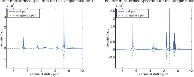
Figure 1: The Fourier transformed¹H-spectra for the two chemical sample mixtures 1 and 2, see Sec. 6.1, prior to any phase and baseline corrections. The spectra are plotted only for the relevant ppm-intervals.

5.1. Idea of the approach

For the simultaneous optimization we use again the objective function f of Equation (1). In contrast to applying consecutive preprocessing steps, now the spectrum is evaluated by a minimization of f not until the baseline cor- rection is applied. The optimization with respect to the variablesϕ0andϕ1 includes baseline corrections as internal computations. We fix the index set Mbl, which specifies the pure baseline regions of the spectrum, by means of an initial baseline step . There is no benefit to re-compute Mbl in each cycle of the simultaneous optimization as its changes are expected to be marginal, but may cause instabilities.

5.2. The algorithm of SINC

The algorithm of the simultaneous phase and baseline correction (SINC) starts with a given Fourier transformed FID signal d^ft∈Cⁿand reads:

1. An initial phase correction is applied to d according to Sec. 3. The result is denoted by d^pha. 2. The set of baseline indices M_blis computed for d^pha.

3. The simultaneous optimization for the parametersϕ₀ andϕ₁ is started by minimizing the objective function f(ϕ0, ϕ1):

(a) Compute the phase corrected spectrum d^pha=Re(ϕ0, ϕ1).

(b) Compute the baseline u for d^phawith respect to the fixed index set Mbl. (c) Evaluate the objective value f(d^pha−u).

Remark 5.1. The functions giin (1) are applied to normalized spectra d/∥d∥^max. Further, the automatic detection of the baseline intervals is independent of the normalization of d^pha. The resulting baseline correction step is homoge- neous of order 1 with respect to the input data. Thus the resulting algorithm of the automated and simultaneous phase and baseline correction is independent of the signal scaling. Thus the weighting parametersγiin (1) do not have to be scaled with a changing amplitude of the data.

5.3. Impact and selection of the control parameters

The SINC algorithm works with various control parameters. In the objective function (1) the Lagrange multipliers γ1,γ2andγ3determine the relative weighting of the constraint functions. Most important is the nonnegativity of the data so thatγ1has to be larger thanγ2, γ3. Reasonable values are given in Section 2. The parameterε1 in g1is the acceptance level for relative negative entries. For medium up to large noise levels a maximal value ofε1 =0.05 is suggested in order to allow for larger negative (noise-)entries. A similar parametrization is suggested forε2, which controls noisy or shifted baselines in the regularization function g₂.

The baseline detection is a crucial part of the SINC method. The degree of the polynomial used by the Savitzky- Golay filter should be small, e. g. ℓ ∈ {1,3}. The band-width parameter m₁ depends mainly on the number n of channels but also on the width of the peaks. Typical values m1 ∈{10, . . . ,30}are suggested if n is large. For small n we use m1 ≤10. The value m2controls the band width for the comparison process in order to decide whether or not a channel belongs to a pure baseline interval. A typical choice for m2is m2 =2m1. Further decisive parameters for the detection of pure baseline intervals areαcrit andδcrit. Ifαcritis large, then more channels are considered for the baseline correction. Ifαcrit =1, then all channels are declared as pure baseline intervals which is not acceptable.

The other extreme isαcrit=0 which means that no baseline correction can be applied. For data including low up to medium noise levels we useαcrit∈{0.3,0.95}. For a higher noise level we suggestαcrit≤0.7. The parameterδcritis closely linked toαcrit. A large value ofδcritincreases the length of pure baseline intervals. For data including a low or a medium noise level we useδcrit∈{1.0,2.0}. For a higher noise level we suggestδcrit≤1.25.

The actual correction of the baseline is controlled by the Lagrange multiplierλ. If the pure baseline intervals are determined properly, then we useλ ∈ [10⁻²,10⁶]and observe only a minor impact of the choice ofλ on the computational results.

6. Numerical results for experimental NMR spectra

Next the new method is tested for experimental NMR spectra. We compare the results of the new simultaneous preprocessing not only with the results of consecutive phase and baseline corrections, but also with an exclusive phase correction. We also compare the results with the entropy minimization approach [4] and the two-stages-tuning as introduced in [1]. The program codes of these two methods are combined with the adaptive iteratively re-weighted penalized least squares approach from [9, 11]. We have applied these methods with and also without their baseline correction algorithms. Additonally we have applied the software package Mnova by Mestrelab.

6.1. Experimental NMR spectra

The¹H NMR spectra of the first two sample mixtures are taken with a medium field NMR spectrometer (Spinsolve Carbon, Magritek, Wellington/New Zealand) using a 1 Tesla permanent magnet so that the proton Larmor frequency equals 42.5 MHz. The spectra are taken with a flip angle of 90^○, a repetition time of 30 s, a number of 32 scans and an acquisition time of 6.4 s. The Fourier transformed FID contains a number of n=65 536 data points. The¹³C spectrum for sample mixture 3 is taken with a Bruker Ascend 400 MHz (console Avance 3 HD 400, probe CyroProbe Prodigy, Bruker Biospin, Rheinstetten/Germany) NMR spectrometer using a 9.4 Tesla vertical superconducting magnet with a proton Larmor frequency of 400.25 MHz. The spectrum is taken with a¹³C inverse gated pulse sequence, a flip angle of 60^○, a relaxation delay of 100 s, a number of 512 scans, and an acquisition time of 1.36 s.

Sample mixture 1. The¹H NMR spectrum is taken from a sample containing 0.66 g of 2-propanol (Sigma-Aldrich, anhydrous,≥ 99.5 mass-%) and 0.266 g of toluene (Merck, Uvasol,≥ 99.9 mass-%). The resulting mole fractions of 2-propanol (PrOH) and toluene (Tol) in the mixture are: xPrOH =0.7918±0.0007 mol/mol and xTol =0.2082± 0.0007 mol/mol, respectively. The real and the imaginary parts of the Fourier transformed spectrum are presented in the left subplot of Fig. 1.

Sample mixture 2. The ¹H NMR spectrum is taken from a sample containing 0.594 g of ethyl acetate (Sigma- Aldrich,≥99.5 mass-%) and 0.428 g of toluene (Merck, Uvasol,≥99.9 mass-%). The resulting mole fractions of ethyl acetate (EtAc) and toluene in the mixture arẽx_EtAc=0.5921±0.0008 mol/mol and̃x_Tol=0.4079±0.0008 mol/mol, respectively. The real and the imaginary parts of the Fourier transformed spectrum are shown in the right subplot of Fig. 1.

8

0 2

4 0 6

0.5 1 1.5 2 2.5 3 3.5

x 10⁷

chemical shift/ppm

intensity/a.u.

0 2

4 6

0 2 4 6 8 10x 10⁵

chemical shift/ppm

intensity/a.u.

zoom along the intensity axis

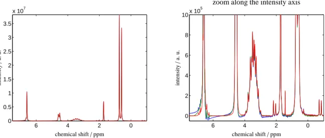
Figure 2: NMR spectra for the binary mixture of 2-propanol and toluene, see the sample mixture 1, after application of three forms of data preprocessing. Left: the NMR spectrum on the relevant 7–(-1) ppm range. Right: zoom along the ordinate-direction. The blue spectrum results from exclusive application of the phase correction, and the green spectrum is the outcome of a consecutive application of the phase and baseline correction steps. The new simultaneous phase and baseline correction algorithm yields the red spectrum. Obviously the best spectrum results from the simultaneous correction algorithm.

Sample mixture 3. The¹³C NMR spectrum is taken from a sample containing 0.09040±0.0001 mol/mol of N- Methyldiethanolamine (Sigma-Aldrich,≥ 99 mass-%), 0.0099±0.0001 mol/mol of sodium carbonate (Th. Geyer,

≥99.8 mass-%), 15.0083 g of water (deionized and purified with a water purification system (Milli-Q Reference A+

System, Merck Millipore, Billerica/US-MA)). Sodium carbonate was dried for 12 h at 120 °C before using and all other chemicals were used without further purification. For details on the sample see [2].

The uncertainties of all mole fractions of the components in the two sample mixtures are estimated from the given accuracy of the laboratory balance and the uncertainties of the purities of the samples.

6.2. Application of the phase and baseline corrections

The NMR spectra for the two mixtures as described in the sample mixture 1 and 2 are subjected to three different preprocessing methods. The control parameters for these computations, namely the weight factorsγi and the trun- cation parametersεi, are already given in Sec. 2. The preprocessed NMR spectra are plotted in Figs. 2 and 3. The blue spectrum results from an application of only the phase correction to either the NMR spectrum of the 2-propanol mixture with toluene, see Fig. 2, or to the NMR spectrum of the ethyl acetate mixture with toluene, see Fig. 3. Espe- cially for the largest peaks some positive dispersion is still present. The green spectra in these two figures represent the results of a consecutive application of the phase and baseline correction steps. The new simultaneous phase and baseline correction algorithm yields in Fig. 2 and in Fig. 3 the red spectrum. The Pareto optimal solution of the simultaneous correction is always the best correction.

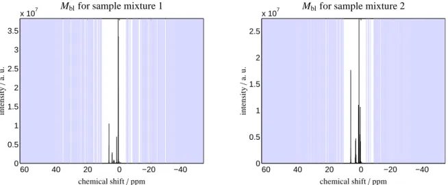
Fig. 4 shows the pure baseline regions in blue color along the complete chemical shift axis for the two sample mixtures. As explained in Sec. 4.3 it is of crucial importance that the index sets are not too large. It is much better to omit some data points of pure baseline regions (which are then filled by linear interpolation) than to assign data points at peak flanks incorrectly to the baseline. This would result in significant distortions of the spectrum, see Sec. 4.4.

Fig. 5 shows a comparison of the four preprocessing methods for sample mixture 3. These methods are the simultaneous phase and baseline correction (SINC), the entropy minimization approach [4] including a simple base- line correction and the two-stages tuning [1] including a simple baseline correction. We also corrected the spectrum with standard algorithms provided in the software package Mnova (Mestrelab, Santiago de Compostela, Spain). For brevity, this method will be called Mnova in the following. In Mnova we applied for the phase correction the automatic consecutive algorithms ”Global”, ”Minimum Entropy”, ”Selective”, ”Baseline Optimization”, ”Metabonomics”, ”Re- gion Analysis”, and ”Whitening”. We also used the settings ”Filter: Autodetect” and ”Smooth Factor: Autodetect”

0 2

4 6

0 8 0.5 1 1.5 2 2.5

x 10⁷

chemical shift/ppm

intensity/a.u.

0 2

4 6

8 0 5 10 15 20x 10⁵

chemical shift/ppm

intensity/a.u.

zoom along the intensity axis

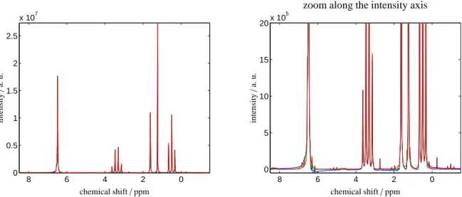
Figure 3: NMR spectra for the ethyl acetate mixture with toluene, see the sample mixture 2, after application of three forms of data preprocessing.

Left: the NMR spectrum on the relevant 8.5–(-1.5) ppm range. Right: zoom along the ordinate-direction. The blue spectrum results from exclusive application of the phase correction, and the green spectrum is the outcome of a consecutive application of the phase and baseline correction steps.

The new simultaneous phase and baseline correction algorithm yields the red spectrum. As in Fig. 2 the best results are obtained by the simultaneous correction algorithm.

for the consecutive baseline correction. The results gained by SINC and Mnova are almost identical. A detail enlarge- ment of the peak close to 167.9 ppm shows small deviations of the results of these two methods compared to entropy minimization and two-stages tuning.

Remark 6.1. The SINC method, the entropy minimization approach and also the two-stages-tuning method use the Fourier transformed FID signal as the data input for the their respective preprocessing steps. In contrast to this, the highly elaborated and powerful Mnova software typically takes the raw FID signal as input and additionally applies FID preprocessing steps as drift correction, apodization, zero filling, linear prediction and further steps. For the purpose of comparison we imported the Fourier transformed FID signal to Mnova and applied its preprocessing steps. We are aware that this does not capitalize the full strength of data preprocessing implemented in Mnova.

6.3. Verification of the results

The gravimetric values on the portions of NMR-resonant hydrogen nuclei in the sample mixtures 1 and 2 are used in order to verify the results of the new method, cf. [18]. To this end we have to know which peaks belong to which of the two chemical compounds in the respective mixture. Then the integrals for the single peaks as well as their relations are computed. Finally the deviations to the expected gravimetric values are calculated. These integral calculations are also executed for the spectra which result from an exclusive application of the phase correction and also for the spectra which result from a consecutive application of the phase and baseline correction steps. Additionally, we apply this comparative gravimetric analysis to the spectra which are attained by the entropy minimization approach [4], the two-stages-tuning method [1] and Mnova.

The gravimetric analysis is first applied to the sample mixture 1. We consider only the peaks or peak group which are centered at 0.66, 1.7, 3.5, 4.6 and 6.6 ppm. The second and the fifth peak group belong to toluene and the remaining ones belong to 2-propanol. The numbers of the associated protons are p=[6,3,1,1,5]. The following chemical shift intervals are used for the integration:

µ1=[0.3,0.9]ppm, µ2=[1.5,1.9]ppm, µ3=[2.8,4.0]ppm, µ4=[4.2,5.0]ppm, µ5=[6.0,7.1]ppm.

For the sample mixture 1 we consider six verification valuesδi=x^NMR_i −xTolfor i=1, . . . ,6. The index i represents the different combinations of peak areas Ajthat can be applied to calculate the mole fraction x^NMR_i . The index j runs

10

−40

−20 0 20 40 060

0.5 1 1.5 2 2.5 3 3.5

x 10⁷

chemical shift/ppm

intensity/a.u.

Mblfor sample mixture 1

−40

−20 0 20 40 060

0.5 1 1.5 2 2.5

x 10⁷

chemical shift/ppm

intensity/a.u.

Mblfor sample mixture 2

Figure 4: The automatically detected pure baseline intervals are colored blue (along the ordinate) for the two sample mixtures 1 and 2.

50 100

0 150 0.5

1 1.5

2x 10⁵

chemical shift/ppm

intensity/a.u.

SINC method entr. min.

Mnova

two-stages tuning

58.3 58.4 58.5 58.6 0 58.7

0.5 1 1.5

2x 10⁵

chemical shift/ppm

intensity/a.u.

Zoom at twin peaks

167.8 167.9

168 168.1

0 0.5 1 1.5 2 2.5

x 10⁴

chemical shift/ppm

intensity/a.u.

Zoom at isolated peak

Figure 5: The four preprocessing methods are compared for the sample mixture 3. The color code is as follows: the new SINC-method (blue), the entropy minimization approach [4] including a simple baseline correction (green), the two-stages-tuning method [1] including a simple baseline correction (cyan) and Mnova (red). Mnova is directly applied to the Fourier transformed FID signal, see Remark 6.1. SINC and Mnova yield nearly the same results, whereas the other two methods show small deviations especially for the peak close to 167.9 ppm.

through the five chemical shift intervals. We calculate the following combinations of the mole fraction of toluene:

x^NMR₁ =A2/(A1+A2), x^NMR₂ =A2/(A3+A2), x^NMR₃ =A2/(A4+A2), x^NMR₄ =A₅/(A₁+A₅), x^NMR₅ =A₅/(A₃+A₅), x^NMR₆ =A₅/(A₄+A₅).

Therein the A_jare A_j=I(d^final(µj))/p_j, i= j, . . . ,5, where I(d^final(µi))is a numerical approximation of the peak area in spectrum d^finalon the integration intervalµiwhich is divided by the number of the associated protons p_i.

The gravimetric analysis is also applied to the sample mixture 2 with the six verification values̃δi=̃x_i^NMR−̃xTol. For this example the selected peak groups are contained in the chemical shift intervals

̃

µ1=[0.2,0.8]ppm, ̃µ2=[0.9,1.4]ppm, ̃µ3=[1.5,1.8]ppm, ̃µ4=[3.0,3.8]ppm, ̃µ5=[6.0,7.0]ppm.

The associated numbers of protons for these five peak groups are p= [3,3,3,2,5]. The peaks in the intervals̃µ1,

̃µ2and̃µ4belong to ethyl acetate, and the peaks iñµ3and̃µ5 belong to toluene. Thẽx_i^NMRfor this mixture are as follows:

̃x₁^NMR=A3/(A1+A3) ̃x₂^NMR=A3/(A2+A3), ̃x₃^NMR=A3/(A4+A3),

̃x₄^NMR=A5/(A1+A5), ̃x₅^NMR=A5/(A2+A5), ̃x₆^NMR=A5/(A4+A5).

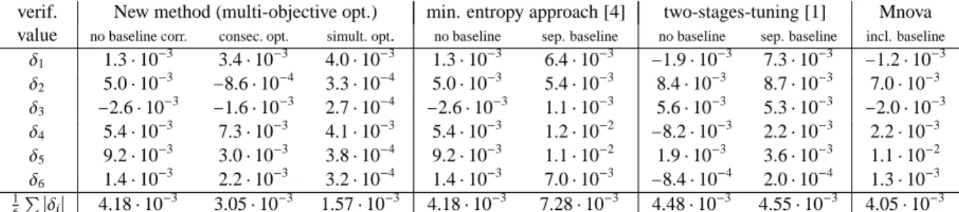
verif. New method (multi-objective opt.) min. entropy approach [4] two-stages-tuning [1] Mnova value no baseline corr. consec. opt. simult. opt. no baseline sep. baseline no baseline sep. baseline incl. baseline

δ1 1.3⋅10⁻³ 3.4⋅10⁻³ 4.0⋅10⁻³ 1.3⋅10⁻³ 6.4⋅10⁻³ −1.9⋅10⁻³ 7.3⋅10⁻³ −1.2⋅10⁻³

δ2 5.0⋅10⁻³ −8.6⋅10⁻⁴ 3.3⋅10⁻⁴ 5.0⋅10⁻³ 5.4⋅10⁻³ 8.4⋅10⁻³ 8.7⋅10⁻³ 7.0⋅10⁻³

δ3 −2.6⋅10⁻³ −1.6⋅10⁻³ 2.7⋅10⁻⁴ −2.6⋅10⁻³ 1.1⋅10⁻³ 5.6⋅10⁻³ 5.3⋅10⁻³ −2.0⋅10⁻³

δ4 5.4⋅10⁻³ 7.3⋅10⁻³ 4.1⋅10⁻³ 5.4⋅10⁻³ 1.2⋅10⁻² −8.2⋅10⁻³ 2.2⋅10⁻³ 2.2⋅10⁻³

δ5 9.2⋅10⁻³ 3.0⋅10⁻³ 3.8⋅10⁻⁴ 9.2⋅10⁻³ 1.1⋅10⁻² 1.9⋅10⁻³ 3.6⋅10⁻³ 1.1⋅10⁻²

δ6 1.4⋅10⁻³ 2.2⋅10⁻³ 3.2⋅10⁻⁴ 1.4⋅10⁻³ 7.0⋅10⁻³ −8.4⋅10⁻⁴ 2.0⋅10⁻⁴ 1.3⋅10⁻³

1

6∑ ∣δi∣ 4.18⋅10⁻³ 3.05⋅10⁻³ 1.57⋅10⁻³ 4.18⋅10⁻³ 7.28⋅10⁻³ 4.48⋅10⁻³ 4.55⋅10⁻³ 4.05⋅10⁻³ Table 1: The table lists the verification valuesδi, i=1, . . . ,6, which are the deviations from the numerical integration approximations from the gravimetric value 0.2082 mol/mol. Eight different preprocessing techniques are considered. The new simultaneous multi-objective optimization in the fourth column gains in most instances the smallest error. The last row contains the mean values of the absolute verification values. Mnova is directly applied to the Fourier transformed FID signal, cf. Remark 6.1.

verif. New method (multi-objective opt.) min. entropy approach [4] two-stages-tuning [1] Mnova value no baseline corr. consec. opt. simult. opt. no baseline sep. baseline no baseline sep. baseline incl. baseline

̃δ1 −7.9⋅10⁻³ −3.9⋅10⁻³ 1.2⋅10⁻⁴ −7.9⋅10⁻³ −2.0⋅10⁻³ −2.0⋅10⁻² −1.1⋅10⁻² −7.4⋅10⁻³

̃δ2 −5.5⋅10⁻³ −4.1⋅10⁻³ 1.6⋅10⁻⁴ −5.6⋅10⁻³ −3.4⋅10⁻³ −1.2⋅10⁻² −1.4⋅10⁻² −4.0⋅10⁻³

̃δ3 −7.9⋅10⁻⁴ −3.4⋅10⁻³ −1.1⋅10⁻³ −8.0⋅10⁻⁴ −2.5⋅10⁻⁴ −1.3⋅10⁻² −2.4⋅10⁻³ 5.0⋅10⁻³

̃δ4 −3.0⋅10⁻³ 1.9⋅10⁻³ 4.1⋅10⁻⁴ −3.0⋅10⁻³ 5.8⋅10⁻³ −9.3⋅10⁻³ 1.0⋅10⁻¹ −9.9⋅10⁻³

̃δ5 −6.3⋅10⁻⁴ 1.7⋅10⁻³ 4.5⋅10⁻⁴ −6.5⋅10⁻⁴ 4.4⋅10⁻³ −1.2⋅10⁻³ 1.0⋅10⁻¹ −6.5⋅10⁻³

̃δ6 4.1⋅10⁻³ 2.4⋅10⁻³ −8.0⋅10⁻⁴ 4.1⋅10⁻³ 7.6⋅10⁻³ −1.8⋅10⁻³ 1.1⋅10⁻¹ 2.4⋅10⁻³

1

6∑ ∣̃δi∣ 3.66⋅10⁻³ 2.90⋅10⁻³ 5.03⋅10⁻⁴ 3.68⋅10⁻³ 3.92⋅10⁻³ 9.70⋅10⁻³ 5.78⋅10⁻² 5.87⋅10⁻³ Table 2: The table lists the verification values̃δi, i=1, . . . ,6, which are the deviations from the numerical integration approximations from the the gravimetric value 0.4079 mol/mol. Eight different preprocessing techniques are considered. The new simultaneous multi-objective optimization in the fourth column gains in most instances the smallest error. The last row contains the mean values of the absolute verification values. Mnova is directly applied to the Fourier transformed FID signal, cf. Remark 6.1.

Remark 6.2. Some entries of the preprocessed spectra can be negative especially if only a phase correction is applied, see e.g. the blue spectra in Figs. 2 and 3. All negative entries are set to zero prior to the numerical integration process in order to avoid major errors - but there is no necessity for this cut-offof negative entries.

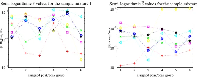
Table 1 lists the verification values for the sample mixture 1 for eight different preprocessing techniques. The analogous values for the sample mixture 2 are given in Table 2. Figure 6 is a semi-logarithmic plot of all these verification values. The final conclusion is:

1. The phase correction approach as used here is very similar to the one presented in [4] on the basis of an entropy minimization (see the columns 1 and 4 in the Tables 1 and 2).

2. The simultaneous phase and baseline correction by multi-objective optimization produces the best results for the given experimental NMR spectra. The separate baseline correction step improves in all cases the results for previous phase correction steps. The smallest deviations in the gravimetric analysis are observed for the simultaneous correction scheme.

7. Conclusion

Competing or even conflicting objectives arise in many optimization problems. In most cases such optimization problems cannot successfully be solved by optimizing each objectives in a step-by-step manner as no single solution can be found which simultaneously optimizes all constraints. Instead, a trade-offis needed between the objectives.

The new algorithm for the phase and baseline correction of NMR spectra demonstrates how the multi-objective opti- mization methodology improves the data preprocessing for NMR data. A characteristic trait of the suggested algorithm is that the detection of pure baseline regions is done only in an initial phase.

12

1 2 3 4 5 6 10⁻⁴

10⁻³ 10⁻²

assigned peak/peak group

∣δ∣inmol/mol

Semi-logarithmicδvalues for the sample mixture 1

1 2 3 4 5 6

10⁻⁴ 10⁻³ 10⁻² 10⁻¹

assigned peak/peak group

∣δ∣inmol/mol

Semi-logarithmic̃δvalues for the sample mixture 2

Figure 6: The deviationsδifrom the gravimetric values 0.2082 mol/mol and the deviations̃δi from 0.4079 mol/mol for the eight different pre- processing methods. The numerical values are listed in Tables 1 and 2. The color code is as follows: (○) for the new method but only with a phase correction, (×) for consecutive phase and baseline corrections by the new method, and (+) for the simultaneous phase correction by the multi-objective optimization. Further, (⊳) represent only the phase correction by minimum entropy approach, (⊲) for the minimum entropy ap- proach with a separate baseline correction step, (◻) for only the phase correction by the two-stages-tuning approach, (◇) for the two-stages-tuning approach with a separate baseline correction step and (☆) for the phase and baseline correction by Mnova. Mnova is directly applied to the Fourier transformed FID signal, cf. Remark 6.1.

The new method is tested for two NMR spectra and shows clear improvements compared to a consecutive op- timization. In a following paper we plan to present an extensive and systematic comparison for various data sets.

Further algorithmic variations, e.g. the use of wavelets for the detection of the pure baseline regions, are possible and the topic of future research.

Acknowledgment

We thank Dan Holland and Yevgen Matviychuk from the University of Canterbury in New Zealand for fruitful discussions. E. von Harbou and K. Neymeyr acknowledge the financial support of the present study by the Deutsche Forschungsgemeinschaft DFG. The project number of von Harbou is HA 7582/1-1.

References

[1] Q. Bao, J. Feng, L. Chen, F. Chen, Z. Liu, B. Jiang, and C. Liu. A robust automatic phase correction method for signal dense spectra. J.

Magn. Reson., 234:82–89, 2013.

[2] R. Behrens, E. von Harbou, W.R. Thiel, W. B¨ottinger, T. Ingram, G. Sieder, and H. Hasse. Monoalkylcarbonate formation in methyldiethanolamine–H2O–CO2. Ind. Eng. Chem. Res., 56(31):9006–9015, 2017.

[3] A. Br¨acher, R. Behrens, E. von Harbou, and H. Hasse. Application of a new micro-reactor¹H NMR probe head for quantitative analysis of fast esterification reactions. Chem. Eng. J., 306:413–421, 2016.

[4] L. Chen, Z. Weng, L. Goh, and M. Garland. An efficient algorithm for automatic phase correction of NMR spectra based on entropy minimization. J. Magn. Reson., 158:164–168, 2002.

[5] J.C. Cobas, M.A. Bernstein, M. Mart´ın-Pastor, and P.G. Tahoces. A new general-purpose fully automatic baseline-correction procedure for 1D and 2D NMR data. J. Magn. Reson., 183(1):145–151, 2006.

[6] E.C. Craig and A.G. Marshall. Automated phase correction of FT NMR spectra by means of phase measurement based on dispersion versus absorption relation (DISPA). J. Magn. Reson, 76(3):458–475, 1988.

[7] H. de Brouwer. Evaluation of algorithms for automated phase correction of NMR spectra. J. Magn. Reson., 201(2):230–238, 2009.

[8] J. Dennis, D. Gay, and R. Welsch. An adaptive nonlinear least-squares algorithm. ACM Transactions on Mathematical Software, 7:348–368, 1981.

[9] P.H.C. Eilers. A perfect smoother. Anal. Chem., 75(14):3631–3636, 2003.

[10] R.R. Ernst. Nuclear magnetic resonance Fourier transform spectroscopy (Nobel Lecture). Angewandte Chemie International Edition in English, 31(7):805–823, 1992.

[11] Gan F., G. Ruan, and J. Mo. Baseline correction by improved iterative polynomial fitting with automatic threshold. Chemom. Intell. Lab.

Syst., 82:59–65, 2006.

[12] S. Golotvin and A. Williams. Improved Baseline Recognition and Modeling of FT NMR Spectra. J. Magn. Reson., 146(1):122–125, 2000.