Including the efficacy of land ice changes in deriving climate sensitivity from paleodata

(1)

https://doi.org/10.5194/esd-10-333-2019

Including the efficacy of land ice changes in deriving climate sensitivity from paleodata

Lennert B. Stap, Peter Köhler, and Gerrit Lohmann

Alfred-Wegener-Institut, Helmholtz-Zentrum für Polar- und Meeresforschung, Am Handelshafen 12, 27570 Bremerhaven, Germany

Correspondence:Lennert B. Stap (lennert.stap@awi.de) Received: 5 December 2018 – Discussion started: 17 December 2018 Revised: 9 May 2019 – Accepted: 27 May 2019 – Published: 14 June 2019

Abstract. The equilibrium climate sensitivity (ECS) of climate models is calculated as the equilibrium global mean surface air warming resulting from a simulated doubling of the atmospheric CO₂concentration. In these simulations, long-term processes in the climate system, such as land ice changes, are not incorporated. Hence, climate sensitivity derived from paleodata has to be compensated for these processes, when comparing it to the ECS of climate models. Several recent studies found that the impact these long-term processes have on global temperature cannot be quantified directly through the global radiative forcing they induce. This renders the prevailing approach of deconvoluting paleotemperatures through a partitioning based on radiative forcings inac- curate. Here, we therefore implement an efficacy factorε_[LI]that relates the impact of land ice changes on global temperature to that of CO₂changes in our calculation of climate sensitivity from paleodata. We apply our refined approach to a proxy-inferred paleoclimate dataset, usingε[LI]=0.45^+0.34_−0.20based on a multi-model assemblage of simulated relative influences of land ice changes on the Last Glacial Maximum temperature anomaly. The imple- mentedε[LI]is smaller than unity, meaning that per unit of radiative, forcing the impact on global temperature is less strong for land ice changes than for CO2changes. Consequently, our obtained ECS estimate of 5.8±1.3 K, where the uncertainty reflects the implemented range inε[LI], is∼50 % higher than when differences in efficacy are not considered.

1 Introduction

Equilibrium climate sensitivity (ECS) expresses the simulated equilibrated surface air temperature response to an in- stantaneous doubling of the atmospheric CO2concentration.

The simulated effect of the applied CO2 radiative forcing anomaly includes the Planck response, as well as the fast feedbacks such as those involving changes to snow, sea ice, lapse rate, clouds, and water vapour. ECS varies significantly between different state-of-the-art climate models; for instance, the CMIP5 ensemble shows a range of 1.9 to 4.4 K (Vial et al., 2013). Several ways have been put forward to constrain ECS, for example, through the use of paleoclimate data (e.g. Covey et al., 1996; Edwards et al., 2007), which is also the focus of this study. However, unlike results of models, temperature reconstructions based on paleoclimate proxy data always contain a mixed signal of all processes active in

the climate system. Among these are long-term processes (or slow feedbacks) such as changes in vegetation, dust, and, ar- guably most importantly, land ice changes, which are kept constant in the climate model runs used to calculate ECS.

Therefore, it is necessary to correct paleotemperature records for the influence of these processes, in order to make a mean- ingful comparison to ECS calculated by climate models.

In a coordinated community effort, the PALAEOSENS project proposed to relate the temperature response caused by these long-term processes to the globally averaged radiative forcing they induce (PALAEOSENS Project Mem- bers, 2012). Consequently, the paleotemperature record can be disentangled on the basis of the separate radiative forcings of these long-term processes (e.g. von der Heydt et al., 2014; Martínez-Botí et al., 2015; Köhler et al., 2015a, 2017b, 2018; Friedrich et al., 2016). If all processes are accounted for in this manner, the effect of CO₂ changes and the ac-

(2)

companying short-term feedbacks, as described by the ECS, can be estimated. However, several studies have shown that, depending on the type of radiative forcing, the same global- average radiative forcing can lead to different global temperature changes (e.g. Stuber et al., 2005; Hansen et al., 2005;

Yoshimori et al., 2011). For instance, in a previous article (Stap et al., 2018a), we simulated the separate and combined effects of CO₂changes and land ice changes on global surface air temperature using the intermediate-complexity climate model CLIMBER-2 and showed that the specific global temperature change per unit radiative forcing change de- pends on which process is involved. As a possible solution to this problem, Hansen et al. (2005) formulated the concept of “efficacy” factors, which express the impact of radiative forcing by a certain process in comparison to the effect of radiative forcing by CO2changes.

Based on the concept of Hansen et al. (2005), here we introduce an efficacy factor for radiative forcing by albedo changes due to land ice variability in our method of deriving climate sensitivity from paleodata. We first illustrate our refined approach by applying it to transient simulations over the past 5 Myr using CLIMBER-2 (Stap et al., 2018a), ob- taining a quantification of the effect on global temperature of CO₂changes and the accompanying short-term feedbacks from a simulation forced by both land ice and CO₂changes.

We compare this result to a simulation where CO₂changes are the only operating long-term process. In this manner, we can assess the error resulting from using a constant efficacy factor. Thereafter, we refine a previous estimate of climate sensitivity based on a paleoclimate dataset of the past 800 kyr (Köhler et al., 2015a, 2018). In this dataset, the sole effect of CO₂is not a priori known. We therefore investigate the influence of the introduced efficacy factor on the calculated climate sensitivity. To do so, we appraise the influence of land ice changes and the associated efficacy using a range that is given by different modelling efforts of the Last Glacial Maxi- mum (LGM;∼21 kyr ago) (Shakun, 2017). The climate sensitivity resulting from applying this range provides a quantification of the consequence of the uncertain efficacy of land ice changes.

2 Material and methods

In this section, we first summarize the approach to obtain- ing climate sensitivity from paleodata that has been used in numerous earlier studies (e.g. PALAEOSENS Project Mem- bers, 2012; von der Heydt et al., 2014; Martínez-Botí et al., 2015; Köhler et al., 2015a, 2017b, 2018; Friedrich et al., 2016). We then discuss our main refinement to that approach, which is the inclusion of the efficacy of land ice changes, and a further small refinement that is meant to unify the dependent variable in cross-plots of radiative forcing and global temperature anomalies.

2.1 Approach to obtain climate sensitivity from paleodata

In climate model simulations used to quantify ECS, fast feedbacks, i.e. processes in the climate system with timescales of less than∼100 years, are accounted for. However, slower processes, such as those involving changes to ice sheets, vegetation, and dust, are commonly kept constant. The resulting response is also sometimes called Charney sensitivity (Char- ney et al., 1979). Following the notation of PALAEOSENS Project Members (2012), the ratio of the temperature change (1T_[CO₂]) to the radiative forcing due to the CO₂ change (1R_[CO₂]) yieldsS^a(in K W⁻¹m², and where “a” stands for actuo):

S^a= 1T_[CO₂]

1R_[CO₂]

. (1)

The subscript denotes that CO₂is the only long-term process involved. Analogously, paleoclimate sensitivity (S^p) can be deduced from paleotemperature reconstructions and paleo- CO₂records as

S^p= 1T_g 1R_[CO₂]

. (2)

In this case, the average global paleotemperature anomaly with respect to the pre-industrial period (PI) (1T_g) is, however, also affected by the long-term processes that are typ- ically neglected in climate simulations. Therefore, a cor- rection to the paleotemperature record is needed to obtain 1T[CO₂]from1Tg:

1T_[CO₂]=1T_g(1−f), (3) or equivalentlyS^afromS^p:

S^a=S^p(1−f)= 1Tg

1R_[CO₂]

(1−f). (4)

Here,f represents the effect of the slow feedbacks on paleotemperature (e.g. van de Wal et al., 2011). To obtainf, PALAEOSENS Project Members (2012) proposed an approach, which has subsequently been used in numerous studies aiming to constrain climate sensitivity from paleodata (e.g. von der Heydt et al., 2014; Martínez-Botí et al., 2015;

Köhler et al., 2015a, 2017b, 2018; Friedrich et al., 2016) and paleoclimate modelling studies (e.g. PALAEOSENS Project Members, 2012; Friedrich et al., 2016; Chandan and Peltier, 2018). They suggested quantifying the influence of the long- term processes (X) by the radiative forcing change they induce (1R_[X]), relative to the total radiative forcing perturbation:

f = 1R_[X]

1R[CO₂]+1R[X]

=1− 1R_[CO₂]

1R[CO₂]+1R[X]

. (5) Combining Eqs. (4) and (5) and following the PALAEOSENS nomenclature, we can then derive the

(3)

“specific” paleoclimate sensitivityS[CO₂,X], whereXrepre- sents the processes that are accounted for in the calculation off:

S[CO₂,X]= 1Tg

1R_[CO₂]

(1− 1R_[X]

1R_[CO₂]+1R_[X])

= 1T_g

1R[CO₂]+1R_[X] = 1T_g 1R[CO₂,X]

. (6)

If, for instance, only the most important slow feedback in the climate system, namely radiative forcing anomalies induced by albedo changes due to land ice (LI) variability, is taken into account, then one can correctS^pto derive the following specific climate sensitivity:

S_[CO₂_,LI]= 1T_g 1R[CO₂]+1R[LI]

= 1T_g 1R[CO₂,LI]

. (7)

Using this approach, several studies performed a least- squares regression through scattered data from paleotemperature and radiative forcing records (Martínez-Botí et al., 2015; Friedrich et al., 2016; Köhler et al., 2015a, 2017b, 2018) relating1T_gto1R_[CO₂_,LI]in a time-independent manner, from whichS_[CO₂_,LI]could be determined. In the course of those studies, a state dependency ofS_[CO₂_,LI]as function of background climate has been deduced for those data which are best approximated by a non-linear function. Furthermore, the quantification ofS_[CO₂_,LI]for those state-dependent cases has been formalized in Köhler et al. (2017b). A synthesis of estimates of S_[CO₂_,LI] from both colder- and warmer-than- present climates has been compiled by von der Heydt et al.

(2016).

2.2 Refinement 1: taking the efficacy of land ice changes into account

The validity of the PALAEOSENS approach to calculatingf is contingent on the notion that identical global-average radiative forcing changes lead to identical global temperature responses, regardless of the processes involved. However, it has been demonstrated that the horizontal and vertical distribution of the radiative forcing affects the resulting temperature response (e.g. Stuber et al., 2005; Hansen et al., 2005;

Yoshimori et al., 2011; Stap et al., 2018a) because, for example, different fast feedbacks are triggered depending on the location of the forcing. To address this issue, Hansen et al.

(2005) introduced the concept of efficacy factors, which we will explore further in this study. These factors (ε_[X]) relate the strength of the temperature response to radiative forcing caused by a certain process X (1T_[X]/1R_[X]) to a similar ratio caused by CO₂ radiative forcing (1T_[CO₂]/1R_[CO₂]).

This introduction of efficacy requires a reformulation offas f_ε:

fε= ε_[X]1R_[X]

1R_[CO₂]+ε_[X]1R_[X]

=1− 1R[CO₂]

1R[CO₂]+ε[X]1R[X]

, (8)

and hence also ofS[CO₂,X]asS^ε_[CO

2,X]: S_[CO^ε

2,X]= 1T_g

1R[CO₂]+ε_[X]1R_[X]. (9) In these reformulations, where in principleε_[X]can take any value, we introduce the superscriptε. This serves to clearly distinguish these newly derived sensitivities from those of the PALAEOSENS approach, in which efficacy was not taken into account, implying that identical radiative forcing of different processes leads to identical temperature changes.

To calculateS_[CO^ε

2,LI], we constrain the efficacy factor for radiative forcing by land ice changes (ε[LI]), using the following formulation, which is based on but slightly modified from Hansen et al. (2005):

1T[LI]

1R[LI]

=ε_[LI]1T_g−1T_[LI]

1R[CO₂]

. (10)

This leads to ε_[LI]= ω

1−ω

1R_[CO₂]

1R_[LI] , (11)

where ω represents the fractional relative influence of land ice changes on the global temperature change (ω= 1T_[LI]/1T_g). Ifε_[LI]is assumed to be constant in time (see Sect. 3.2), it can be calculated using Eq. (11) from data of any time step in the record of1R[CO₂]and1R[LI], and consequently applied to the whole record (Fig. 1a, c). As before, with thisε[LI]a quantification ofS_[CO^ε

2,LI]can be obtained by performing a least-squares regression through scattered data from paleotemperature and radiative forcing records, now re- lating1Tgto (1R_[CO₂]+ε[LI]1R[LI]) in a time-independent manner.

Note that apart from the formulation based on Hansen et al. (2005) followed here, other formulations of the efficacy factor are possible. For instance, one can define an alternative efficacy factor (ε_[LI],alt) such that it relates the effect of land ice changes on global temperature directly to the radiative forcing anomaly caused by CO₂changes, leading to S_[CO^ε

2,X],alt= 1T_g

1R[CO₂]+ε[LI],alt1R[CO₂]

. (12)

In this alternative case, the efficacy factorε_[LI],alt relates to our originalε[LI]as

ε_[LI],alt=ε_[LI] 1R[LI]

1R_[CO₂]

. (13)

This implies that ifε_[LI]is indeed constant, any non-linearity in the relation between1R_[CO₂]and1R_[LI]would demand a more complex formulation of the alternative efficacy factor ε_[LI],alt (e.g. via a higher-order polynomial). Since we find

(4)

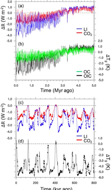
Figure 1.Time series of radiative forcing anomalies (1R) caused by CO₂ (red) changes and land ice changes (blue) and global temperature anomalies (1Tg) with respect to PI from (a–b)the CLIMBER-2 model dataset (Stap et al., 2018a), with temperature data for experiment OIC in black and for experiment OC in green, and from(c–d)the proxy-inferred dataset (Köhler et al., 2015a), with solid lines for the whole dataset and dots for the data used in this study which exclude times with strong temperature–CO₂divergence (see Sect. 4.1). Note the differing axis scales.

such a non-linearity in our data (Fig. 2), using an F test to determine that a second-order polynomial is a significantly (p value<0.0001) better fit to the data than a linear function, we refrain from following this alternative formulation further.

2.3 Refinement 2: unifying the dependent variable To calculate S_[CO^ε

2,LI], previous studies have used cross- plots of global temperature anomalies and radiative forcing. The latter is caused by a combination of CO₂and land ice changes, which is cumbersome if one wants to compare S_[CO^ε

2,LI]to other specific paleoclimate sensitivitiesS_[CO^ε

2,X], where more and/or different long-term processes are considered. Here, we therefore reformulate our quantification of S_[CO^ε

2,LI]to unify the dependent variable as1R_[CO₂]. S_[CO^ε

2,X]= 1T_g

1R_[CO₂]+ε_[X]1R_[X]

= 1Tg

1R_[CO₂]

1R_[CO₂]+ε_[X]1R_[X]

= 1T_[−X]^ε 1R_[CO₂]

(14) Here,1T_[−X]^ε is the global temperature change (with respect to PI) stripped of the inferred influence of processesX, de- fined as

1T_[−X]^ε :=1Tg

1R_[CO₂]

1R_[CO₂]+ε_[X]1R_[X]. (15) Hence, for the calculation ofS_[CO^ε

2,LI], we use 1T_[−LI]^ε :=1T_g 1R[CO₂]

1R[CO₂]+ε[LI]1R[LI]

. (16)

Now, we quantifyS_[CO^ε

2,LI]by performing a least-squares regression (regfunc) through scattered data from1T_[−LI]^ε and 1R_[CO₂]. We use the precondition that no change in CO₂is related to no change in1T_[−LI]^ε , meaning the regression in- tersects they axis at the origin ((x, y)=(0,0)). Following Köhler et al. (2017b), for any non-zero1R_[CO₂], we calcu- lateS_[CO^ε

2,LI]as S_[CO^ε

2,LI]

1R[CO2]

= regfunc 1R[CO₂]

1R[CO2]

. (17)

If1R[CO₂]=0 W m⁻², as is, for instance, the case for pre- industrial conditions,S_[CO^ε

2,LI]is quantified as S_[CO^ε

2,LI]

_1R

[CO2]=0

= δ(regfunc) δ(1R[CO₂])

_1R

[CO2]=0

. (18)

Equations (17) and (18) yield a quantification of S^ε_[CO

2,LI], which can be compared to the value obtained forS_[CO^ε

2,LI]

using the PALAEOSENS approach that does not consider efficacy differences (equivalent to usingε_[LI]=1) (Köhler et al., 2018).

To obtainS^a, one needs to multiplyS_[CO₂_,LI] by a conversion factor φ=0.64±0.07 (1σ uncertainty) that ac- counts for the influence of other long-term processes, namely vegetation, aerosol, and non-CO₂ greenhouse gas changes

(5)

(PALAEOSENS Project Members, 2012). Note that this mul- tiplication byφignores any possible state dependencies inφ and assumes unit efficacy for processes other than land ice changes. Because a comprehensive analysis of the efficacy and state dependency of these other processes is beyond the scope of this study, it is a source of uncertainty to be investigated in future research. Finally, we obtain the equivalent ECS by multiplying S^a by1R_2×CO₂=3.71±0.37 W m⁻² (1σuncertainty), the radiative forcing perturbation represent- ing a CO₂doubling (Myhre et al., 1998).

3 Illustration of the approach using model simulations

In this section, we illustrate our refined approach, which con- siders efficacy differences, by applying it to transient simulations over the past 5 Myr using CLIMBER-2 (Stap et al., 2018a). We obtain a quantification of the effect on global temperature of CO₂ changes and the accompanying short- term feedbacks from a simulation forced by both land ice and CO2changes. We compare this result to a simulation where CO2 changes are the only operating long-term process. By doing so, we assess the error resulting from using a constant efficacy factor.

3.1 CLIMBER-2 model simulations

Currently, long (∼10⁵to∼10⁶years) integrations of state- of-the-art climate models, such as general circulation models and Earth system models, are not yet not feasible due to limited computer power. This gap can be filled by using models of reduced complexity (Claussen et al., 2002;

Stap et al., 2017). Using the intermediate-complexity climate model CLIMBER-2 (Petoukhov et al., 2000; Ganopol- ski et al., 2001), climate simulations over the past 5 Myr were performed and analysed in Stap et al. (2018a). CLIMBER- 2 combines a 2.5-dimensional statistical–dynamical atmosphere model, with a three-basin zonally averaged ocean model (Stocker et al., 1992) and a model that calculates dy- namic vegetation cover based on the temperature and pre- cipitation (Brovkin et al., 1997). The simulations could be forced by solar insolation changes due to orbital (O) variations (Laskar et al., 2004), by land ice (I) changes in both hemispheres (based on de Boer et al., 2013), and by CO2

(C) changes (based on van de Wal et al., 2011). In the ref- erence experiment (OIC) all these factors are varied, while in other model integrations the land ice (experiment OC) or the CO₂ concentration (experiment OI) is kept fixed at PI level. The synergy of land ice and CO₂changes is negligibly small, meaning their induced temperature changes add approximately linearly when both forcings are applied. Further- more, the influence of orbital variations is also very small, so that experiment OC approximately yields the sole effect of CO₂changes on global temperature (1T_[OC]). As in Stap et al. (2018a), we use the simple energy balance model of

Figure 2.The relation between radiative forcing anomalies caused by CO₂changes (1R_[CO₂_]) and land ice changes (1R_[LI]) from the whole proxy-inferred dataset (Köhler et al., 2015a) (pink dots). The red line represents a second-order polynomial least-squares regression through the scattered data.

Köhler et al. (2010) to analyse the applied radiative forcing of land ice albedo and CO2 changes and simulated global temperature changes, after averaging to 1000-year temporal resolution (Fig. 1a, b).

3.2 Analysis

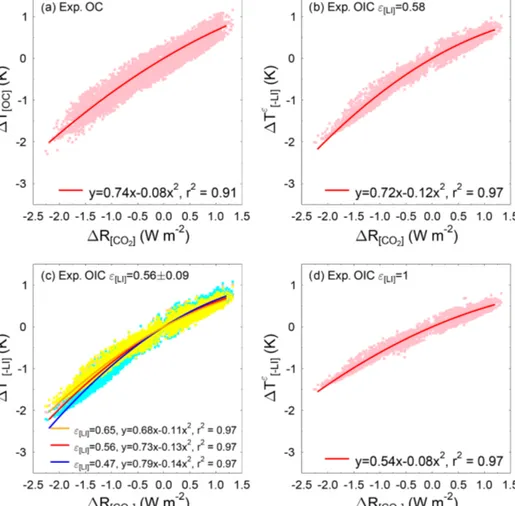
First, we analyse experiment OC, which will serve as a target for our approach as deployed later in this section. We use a least-squares regression through scattered data of1R_[CO₂]

and1T_[OC] to fit a second-order polynomial (Fig. 3a). Us- ing a higher-order polynomial rather than a linear function allows us to capture the state dependency of paleoclimate sensitivity. Fitting even higher-order polynomials leads to negligible coefficients for the higher powers and is not pur- sued further. From the fit, we calculate a specific paleoclimate sensitivityS_[CO^ε

2,LI]of 0.74 K W⁻¹m²for PI conditions (1R_[CO₂]=0 W m⁻²) using Eq. (18). Note that, in this case, S_[CO^ε

2,LI]is equal toS_[CO^ε

2],S_[CO₂_,LI], andS_[CO₂]as there are no land ice changes and therefore also no efficacy differences. The fit further shows decreasingS_[CO^ε

2,LI] for rising 1R[CO₂].

Now, we apply our approach to the results of experiment OIC, in which both CO2 and land ice cover vary over time, with the aim of deducing the sole effect of CO₂ changes on global temperature. We calculate the efficacy of land ice changes for the LGM (21 kyr ago) from experiment OI, in which the CO₂ concentration is kept constant.

We obtainω=1T_[LI]/1T_g=1T_[OI]/1T_[OIC]=0.54. Con- sequently, we findε_[LI]=0.58 from Eq. (11) and apply this value to the whole record of 1R_[CO₂] and 1R_[LI]. In this manner, we calculate1T_[−LI]^ε using Eq. (16). In principle, ε_[LI] can be obtained using data from any time step of the

(6)

record, preferably when the radiative forcing anomalies are large to prevent outliers resulting from divisions by small numbers. For example, using the results from all glacial marine isotope stages of the past 810 kyr (Marine Isotope Stage (MIS) 2, 6, 8, 10, 12, 14, 16, 18, and 20), instead of only the LGM, leads to a mean (±1σ)ε_[LI]of 0.56±0.09.

We then fit a second-order polynomial to the scattered data of the thusly obtained 1T_[−LI]^ε from the results of experiment OIC and 1R_[CO₂] (Fig. 3b, c). Between 1R_[CO₂]=

−0.5 W m⁻² and 1R_[CO₂]=0.5 W m⁻², outliers resulted from division by small numbers (not shown in Fig. 3b). To remove these outliers, we first calculate the root mean square error (RMSE) between the fit and the data in the remainder of the domain. We then exclude all values from the range 1R[CO₂]= −0.5 W m⁻²to1R[CO₂]=0.5 W m⁻², where the fit differs from the data by more than 3 times the RMSE, and perform the regression again. This yields anS_[CO^ε

2,LI]of 0.72 K W⁻¹m² for PI (Fig. 3b) in the LGM-only case and 0.73^+0.06_−0.05K W⁻¹m²in the case where all glacial periods are used (Fig. 3c). This supports our approach since it is only slightly lower than theS_[CO^ε

2,LI]of 0.74 K W⁻¹m²obtained from experiment OC, which it should approximate. The rela- tionship between1T_[−LI]^ε and1R[CO₂](Fig. 3b) is less linear than that between1T[OC]and1R[CO₂](Fig. 3a); hence, the state dependency ofS_[CO^ε

2,LI]is enhanced. However, the difference between theS_[CO^ε

2,LI]obtained from both exper- iments remains smaller than 0.07 K W⁻¹m²throughout the entire 5 Myr interval in the LGM-only case, indicating that a constant efficacy is an acceptable assumption which only introduces a negligible additional uncertainty. However, the possible time dependency of efficacy could be investigated more rigorously in future research using more sophisticated climate models.

The PALAEOSENS approach that does not consider efficacy differences (ε_[LI]=1) yields a PI S_[CO₂_,LI] of 0.54 K W⁻¹m² (Fig. 3d). This is clearly much more off- target than the results of our approach, signifying the impor- tance of considering efficacy.

4 Application to proxy-inferred paleoclimate data In this section, we compare our refined approach to calcu- latingS_[CO^ε

2,LI]incorporating efficacy to our previous quantification of S_[CO₂_,LI] (Köhler et al., 2018) by reanalysing the same paleoclimate dataset (introduced in Köhler et al., 2015a). Other than for climate model simulations, in proxy- based datasets the influence of land ice changes on global temperature perturbations cannot be directly obtained and hence is a priori unknown. We therefore base the value of ε[LI] we implement here on a multi-model assemblage of simulated relative influences of land ice changes on the LGM temperature anomaly (Shakun, 2017).

4.1 Proxy-inferred paleoclimate dataset

The dataset to be investigated contains reconstructions of 1T_g, 1R_[CO₂], and 1R_[LI] for the past 800 kyr. Although the dataset covers the past 5 Myr, here we focus only on the past 800 kyr (Fig. 1c, d) because over this period1R_[CO₂]

is constrained by high-fidelity measurements of CO₂within ice cores, whereas Pliocene and Early Pleistocene CO₂levels are still heavily debated (e.g. Badger et al., 2013; Martínez- Botí et al., 2015; Willeit et al., 2015; Stap et al., 2016, 2017; Chalk et al., 2017; Dyez et al., 2018). Radiative forcing by CO2 is obtained from Antarctic ice core data compiled by Bereiter et al. (2015), using1R[CO₂]=5.35 W m⁻²· ln(CO2/(278 ppm)) (Myhre et al., 1998). The revised formulation for 1R[CO₂] from Etminan et al. (2016) leads to very similar results with less than 0.01 W m⁻² differences between the approaches for typical late Pleistocene CO₂values (Köhler et al., 2017a). Radiative forcing caused by land ice albedo changes, as well as the global surface air temperature record (1T_g), are based on results of the 3-D ice- sheet model ANICE (de Boer et al., 2014) forced by northern hemispheric temperature anomalies with respect to a ref- erence PI climate. The ANICE results are here considered to be proxy-inferred because, unlike climate models, AN- ICE is not constrained by climatic boundary conditions such as insolation and greenhouse gases. The temperature anomalies follow directly from a benthicδ¹⁸O stack (Lisiecki and Raymo, 2005) using an inverse technique. Nevertheless, the results are model-dependent and therefore subject to uncertainty. ANICE provided geographically specific land ice dis- tributions and hence radiative forcing due to albedo changes with respect to PI in both hemispheres. In Köhler et al.

(2015a), the northern hemispheric (NH) temperature anomalies (1T_NH) are translated into global temperature perturbations (1T_g1 in Köhler et al. (2015a)) using polar amplification factors (f_PA=1T_NH/1T_g) as follows: at the LGM, f_PA=2.7 is taken from the average of PMIP3 model data (Braconnot et al., 2012), while at the mid-Pliocene Warm Period (mPWP, about 3.2 Myr ago),f_PA=1.6 is calculated from the average of PlioMIP results (Haywood et al., 2013).

At all other times,fPA is linearly varied as a function of the NH temperature. In Appendix A, we investigate the influence of the chosen polar amplification factor on our results.

The temporal resolution of the dataset is 2000 years.

Analysing this dataset, Köhler et al. (2018) found a temperature–CO₂divergence appearing mainly during, or in connection with, periods of decreasing obliquity related to land ice growth or sea level fall. For these periods, a significantly differentS_[CO₂_,LI]was obtained than for the remainder of the time frame. However, in the future, we expect sea level to rise; hence, these intervals of strong temperature–CO₂divergence should not be considered for the interpretation of paleodata in the context of future warming, e.g. by using paleodata to constrain ECS. In the following analysis, we there-

(7)

Figure 3.Temperature anomalies with respect to PI over the last 5 Myr from CLIMBER-2 (Stap et al., 2018a) against imposed radiative forcing of CO₂.(a)Simulation with fixed PI land ice distribution (experiment OC) (1T_[OC]).(b)Calculated global temperature perturbations from experiment OIC stripped of the inferred influence of land ice (1T_[−LI]^ε ) using Eq. (16) withε_[LI]=0.58. Here,ε_[LI]is obtained from matching climate sensitivity with the target value at the LGM.(c)Same as in panel(b)but usingε_[LI]=0.47 (cyan dots),ε_[LI]=0.56 (pink dots), andε_[LI]=0.65 (yellow dots), Here,ε_[LI]is obtained from the mean (±1σ) of matching climate sensitivity with the target value at all glacial marine isotope stages of the past 810 kyr (MIS 2, 6, 8, 10, 12, 14, 16, 18, and 20).(d)Same as in panel(b)but usingε_[LI]=1, which is equivalent to the PALAEOSENS approach where efficacy differences were not considered. The red lines – and in panel(c)also the orange and blue lines – represent second-order polynomial least-squares regressions through the scattered data.

fore exclude these times with strong temperature–CO2diver- gence, leaving 217 data points as indicated in Fig. 1c, d.

4.2 Analysis

Shakun (2017) compiled model-based estimates of the relative impact of land ice changes on the LGM temperature anomaly (ω in Eq. 11) using an ensemble of 12 climate models and estimated ωto be 0.46±0.14 (mean±1σ; full range 0.20–0.68). Applying these values, in combination with the LGM values (taken here as the mean of the data at 20 and 22 kyr ago) 1R_[CO₂]= −2.04 W m⁻² and1R_[LI]=

−3.88 W m⁻², yields ε_[LI]=0.45^+0.34_−0.20. Implementing this range for ε_[LI] in Eq. (16), we calculate 1T_[−LI]^ε over the whole 800 kyr period. Fitting second-order polynomials by least-squares regression to the scattered data of 1T_[−LI]^ε

and1R[CO₂], we infer a PIS_[CO^ε

2,LI]of 2.45^+0.53_−0.56K W⁻¹m² (Fig. 4a). The substantial uncertainty given here only reflects the 1σ uncertainty inε[LI]. Similar to Köhler et al. (2018), we also detect a state dependency with decreasingS_[CO^ε

2,LI]

towards colder climates for this dataset, more strongly so in the case of lowerε_[LI]. This state dependency is oppo- site to the one found in the CLIMBER-2 results (Sect. 3).

The difference may be related either to the fact that fast climate feedbacks are too linear or that some slow feedbacks are underestimated in intermediate-complexity climate models like CLIMBER-2 (see Köhler et al., 2018, for a detailed discussion). At 1R_[CO₂]= −2.04 W m⁻², the LGM value, S_[CO^ε

2,LI] is only 1.45^+0.33_−0.37K W⁻¹m². The PALAEOSENS approach, which does not consider efficacy and is therefore equivalent to our approach usingε[LI]=1, yieldsS[CO₂,LI]= 1.66 K W⁻¹m²for PI andS[CO₂,LI]=0.93 K W⁻¹m²for the

(8)

Figure 4.The global temperature perturbations stripped of the inferred influence of land ice (1T_[−LI]^ε ) calculated using Eq. (16) against 1R_[CO₂]from the proxy-inferred paleoclimate dataset (Köhler et al., 2015a), using(a)ε_[LI]=0.79 (maroon dots),ε_[LI]=0.45 (cyan dots), andε_[LI]=0.25 (green dots). Here,ε_[LI]is obtained by converting the multi-model assemblage of simulated relative influences of land ice changes on the LGM temperature anomaly (0.46±0.14) (Shakun, 2017).(b)Same as in panel(a)but usingε[LI]=1 (grey dots), which is equivalent to the PALAEOSENS approach. The brown, blue, dark green(a), and black lines(b)represent second-order polynomial least- squares regressions through the data.

LGM (Fig. 4b). The specific paleoclimate sensitivities we find using the refined approach are hence generally larger than those obtained when neglecting efficacy differences.

This is because, for the range of the impact of land ice changes on the LGM temperature anomaly implemented (ω=0.46±0.14), the efficacy factor ε[LI] is smaller than unity. In other words, these land ice changes contribute com- paratively less per unit radiative forcing to the global temperature anomalies than the CO2changes.

Our inferred PI S_[CO^ε

2,LI] is equivalent to an S^a of 1.6^+0.3_−0.4K W⁻¹m² when only considering the uncertainty caused by the implemented range in ε_[LI] and to an S^a of 1.6^+0.1_−0.2K W⁻¹m²when only considering the uncertainty in the conversion factorφ. The equivalent ECS is 5.8±1.3 K per CO2doubling when only considering the uncertainty caused by the implemented range inε[LI] and 5.8±0.6 K per CO2

doubling when only considering the uncertainty in the conversion factor1R2×CO₂. The ECS we find is thus at the high end of the results of other approaches to obtain ECS (Knutti et al., 2017), e.g. the 2.0 to 4.3 K 95 % confidence range from a large model ensemble (Goodwin et al., 2018) and the 2.2 to 3.4 K 66 % confidence range from an emerging constraint from global temperature variability and CMIP5 (Cox et al., 2018). Hence, the low end of our ECS estimate is in the best agreement with these other estimates. This could mean that the relative influence of land ice changes on the LGM temperature anomaly is on the high side of or possibly higher than the 0.46±0.14 range we consider here. Alternatively, the conversion factorφ=0.64±0.07 we use to convertS[CO₂,LI]

toS^ais an overestimation, which could be caused by a larger- than-unity efficacy of long-term processes besides CO2and land ice changes. We have focused primarily on the effect of

ε_[LI]onS_[CO^ε

2,LI]in this analysis, and therefore we have, for simplicity, ignored uncertainties in the investigated proxy- inferred records themselves. A comprehensive description of these uncertainties and their influence on the calculated climate sensitivity can be found in Köhler et al. (2015a).

5 Conclusions

We have incorporated the concept of a constant efficacy factor (Hansen et al., 2005), which interrelates the global temperature responses to radiative forcing caused by land ice changes and CO₂ changes, into our framework of calculat- ing specific paleoclimate sensitivityS_[CO^ε

2,LI]. The aim of this effort has been to overcome the problem that land ice and CO₂ changes can lead to significantly different global temperature responses, even when they induce the same global- average radiative forcing. Firstly, we have assessed the use- fulness of considering efficacy differences by applying our refined approach to results of 5 Myr CLIMBER-2 simulations (Stap et al., 2018a), where the separate effects of land ice changes and CO2changes can be isolated. In the results of these simulations, the error from assuming the efficacy factor to be constant in time is negligible. Thereafter, we have used our approach to reanalyse an 800 kyr proxy-inferred paleoclimate dataset (Köhler et al., 2015a). We have inferred a range in the land ice change efficacy factorε_[LI]from the relative impact of land ice changes on the LGM temperature anomaly simulated by a 12-member climate model ensemble (Shakun, 2017). The thusly obtained efficacy factor ε_[LI]=0.45^+0.34_−0.20is smaller than unity, implying that the impact on global temperature per unit of radiative forcing is less strong for land ice changes than for CO₂changes. Con-

(9)

sequently, our derived PIS_[CO^ε

2,LI]of 2.45^+0.53_−0.56K W⁻¹m²is

∼50 % larger than when efficacy differences are neglected.

The equivalent S^a and ECS corresponding to thisS_[CO^ε

2,LI]

are 1.6^+0.3_−0.4K W⁻¹m²and 5.8±1.3 K per CO₂doubling, re- spectively. The uncertainty in these estimates is only caused by the implemented range inε[LI].

Data availability. The CLIMBER-2 dataset is available at https://doi.org/10.1594/PANGAEA.887427 (Stap et al., 2018b), and the proxy-inferred paleoclimate dataset is available at https://doi.org/10.1594/PANGAEA.855449 (Köhler et al., 2015b).

For more information or data, please contact the authors.

(10)

Appendix A: Influence of the polar amplification factor

In the analysis performed in Sect. 4.2, we used a global temperature record that was obtained from northern high-latitude temperature anomalies using a polar amplification factorfPA

that varies from 2.7 in the coldest to 1.6 in the warmest conditions (Sect. 4.1). However, recent climate model simulations of the Pliocene using updated paleogeographic boundary conditions show that in warmer times polar amplification could have been nearly the same as in colder times (Kamae et al., 2016; Chandan and Peltier, 2017). We therefore re- peat the analysis using the same range inε_[LI]and the same dataset but with an applied constantf_PA=2.7 over the entire past 800 kyr to generate1T_g(1T_g2in Köhler et al., 2015a).

Figure A1.The global temperature perturbations stripped of the inferred influence of land ice (1T_[−LI]^ε ) calculated using Eq. (16) against 1R_[CO₂]from the proxy-inferred paleoclimate dataset (Köhler et al., 2015a), using(a)ε_[LI]=0.79 (maroon dots),ε_[LI]=0.45 (cyan dots), andε[LI]=0.25 (green dots). Here,ε[LI]is obtained from converting the multi-model assemblage of simulated relative influences of land ice changes on the LGM temperature anomaly (0.46±0.14) (Shakun, 2017).(b) Same as in panel(a)but usingε_[LI]=1 (grey dots), which is equivalent to the PALAEOSENS approach. The brown, blue, dark green(a), and black lines(b)represent second-order polynomial least-squares regressions through the data. Here, the global temperature anomalies are derived from the northern high-latitude temperature anomaly reconstruction assuming a constant polar amplification factor (f_PA) of 2.7, as opposed to the variablef_PAused in Fig. 4.

The constant polar amplification used here counteracts in- creasing state dependency towards low temperatures, as the temperature differences are no longer amplified by chang- ing polar amplification. Hence, S_[CO^ε

2,LI] is smaller at PI (1.96^+0.42_−0.44K W⁻¹m² compared to 2.45^+0.53_−0.56K W⁻¹m² using the variable fPA) but diminishes less strongly towards colder conditions (Fig. A1a, cf. Fig. 4a). As before, the PALAEOSENS approach (equivalent to our approach us- ingε[LI]=1) yields a lower PIS[CO₂,LI]of 1.34 K W⁻¹m² (Fig. A1b). The PIS_[CO^ε

2,LI]inferred here using our refined approach corresponds to anS^aof 1.3^+0.2_−0.3K W⁻¹m²and an ECS of 4.6^+1.0_−1.3K per CO2doubling.

(11)

Author contributions. LBS designed the research. LBS and PK performed the analysis. LBS drafted the paper, with input from all co-authors.

Competing interests. The authors declare that they have no con- flict of interest.

Acknowledgements. This work is institutionally funded at AWI via the research program PACES-II of the Helmholtz Association.

We thank Roderik van de Wal for commenting on an earlier draft of the paper and two anonymous referees for their constructive com- ments, which have helped to improve the quality of the paper.

Financial support. The article processing charges for this open- access publication were covered by a Research Centre of the Helmholtz Association.

Review statement. This paper was edited by Daniel Kirk- Davidoff and reviewed by two anonymous referees.

References

Badger, M. P. S., Lear, C. H., Pancost, R. D., Foster, G. L., Bailey, T. R., Leng, M. J., and Abels, H. A.: CO₂drawdown following the middle Miocene expansion of the Antarctic Ice Sheet, Pa- leoceanography, 28, 42–53, https://doi.org/10.1002/palo.20015, 2013.

Bereiter, B., Eggleston, S., Schmitt, J., Nehrbass-Ahles, C., Stocker, T. F., Fischer, H., Kipfstuhl, S., and Chappellaz, J.: Revision of the EPICA Dome C CO₂ record from 800 to 600 kyr before present, Geophys. Res. Lett., 42, 542–549, https://doi.org/10.1002/2014GL061957, 2015.

Braconnot, P., Harrison, S. P., Kageyama, M., Bartlein, P. J., Masson-Delmotte, V., Abe-Ouchi, A., Otto-Bliesner, B., and Zhao, Y.: Evaluation of climate models using palaeoclimatic data, Nat. Clim. Change, 2, 417–424, https://doi.org/10.1038/nclimate1456, 2012.

Brovkin, V., Ganopolski, A., and Svirezhev, Y.: A continuous climate-vegetation classification for use in climate-biosphere studies, Ecol. Model., 101, 251–261, https://doi.org/10.1016/S0304-3800(97)00049-5, 1997.

Chalk, T. B., Hain, M. P, Foster, G. L., Rohling, E. J., Sexton, P.

F., Badger, M. P. S., Cherry, S. G., Hasenfratz, A. P., Haug, G.

H., Jaccard, S. L., Martínez-García, A., Pälike, H., Pancost, R.

D., and Wilson, P. A.: Causes of ice age intensification across the Mid-Pleistocene Transition, P. Natl. Acad. Sci. USA, 114, 13114–13119, https://doi.org/10.1073/pnas.1702143114, 2017.

Chandan, D. and Peltier, W. R.: Regional and global climate for the mid-Pliocene using the University of Toronto version of CCSM4 and PlioMIP2 boundary conditions, Clim. Past, 13, 919–942, https://doi.org/10.5194/cp-13-919-2017, 2017.

Chandan, D. and Peltier, W. R.: On the mechanisms of warming the mid-Pliocene and the inference of a hierarchy of climate sensitivities with relevance to the understanding of climate

futures, Clim. Past, 14, 825–856, https://doi.org/10.5194/cp-14- 825-2018, 2018.

Charney, J. G., Arakawa, A., Baker, D. J., Bolin, B., Dickinson, R. E., Goody, R. M., Leith, C. E., Stommel, H. M., and Wun- sch, C. I.: Carbon dioxide and climate: a scientific assessment, National Academy of Sciences, Washington, DC, 1979.

Claussen, M., Mysak, L., Weaver, A., Crucifix, M., Fichefet, T., Loutre, M.-F. ,Weber, S., Alcamo, J., Alexeev, V., Berger, A., Calov, R., Ganopolski, A., Goosse, H., Lohmann, G., Lunkeit, F., Mokhov, I., Petoukhov, V., Stone, P., and Wang, Z.: Earth system models of intermediate complexity: closing the gap in the spectrum of climate system models, Clim. Dynam., 18, 579–586, https://doi.org/10.1007/s00382-001-0200-1, 2002.

Covey, C., Sloan, L. C., and Hoffert, M. I.: Paleocli- mate data constraints on climate sensitivity: the pale- ocalibration method, Climatic Change, 32, 165–184, https://doi.org/10.1007/BF00143708, 1996.

Cox, P. M., Huntingford, C., and Williamson, M. S.:

Emergent constraint on equilibrium climate sensitivity from global temperature variability, Nature, 553, 319, https://doi.org/10.1038/nature25450, 2018.

de Boer, B., van de Wal, R. S. W., Lourens, L. J., Bintanja, R., and Reerink, T. J.: A continuous simulation of global ice volume over the past 1 million years with 3-D ice-sheet models, Clim. Dy- nam., 41, 1365–1384, https://doi.org/10.1007/s00382-012-1562- 2, 2013.

de Boer, B., Lourens, L. J., and van de Wal, R. S. W.: Persistent 400,000-year variability of Antarctic ice volume and the carbon cycle is revealed throughout the Plio-Pleistocene, Nat. Commun., 5, 2999, https://doi.org/10.1038/ncomms3999, 2014.

Dyez, K. A., Hönisch, B., and Schmidt, G. A.: Early Pleis- tocene obliquity-scale pCO₂variability at ∼1.5 million years ago, Paleoceanography and Paleoclimatology, 33, 1270–1291, https://doi.org/10.1029/2018PA003349, 2018.

Edwards, T. L., Crucifix, M., and Harrison, S. P.: Using the past to constrain the future: how the palaeorecord can improve estimates of global warming, Prog. Phys. Geog., 31, 481–500, https://doi.org/10.1177/0309133307083295, 2007.

Etminan, M., Myhre, G., Highwood, E. J., and Shine, K. P.: Ra- diative forcing of carbon dioxide, methane, and nitrous oxide: A significant revision of the methane radiative forcing, Geophys.

Res. Lett., 43, 542–549, https://doi.org/10.1002/2016GL071930, 2016.

Friedrich, T., Timmermann, A., Tigchelaar, M., Timm, O. E., and Ganopolski, A.: Non-linear climate sensitivity and its impli- cations for future greenhouse warming, Science Advances, 2, e1501923, https://doi.org/10.1126/sciadv.1501923, 2016.

Ganopolski, A., Petoukhov, V., Rahmstorf, S., Brovkin, V., Claussen, M., Eliseev, A., and Kubatzki, C.: CLIMBER- 2: a climate system model of intermediate complexity.

Part II: model sensitivity, Clim. Dynam., 17, 735–751, https://doi.org/10.1007/s003820000144, 2001.

Goodwin, P., Katavouta, A., Roussenov, V. M., Foster, G. L., Rohling, E. J., and Williams, R. G.: Pathways to 1.5^◦C and 2^◦C warming based on observational and geological constraints, Nat.

Geosci., 11, 102–107, https://doi.org/10.1038/s41561-017-0054- 8, 2018.

Hansen, J., Sato, M., Ruedy, R., Nazarenko, L., Lacis, A., Schmidt, G. A., Russell, G., Aleinov, I., Bauer, M., Bauer, S., Bell, N.,

(12)

Cairns, B., Canuto, V., Chandler, M., Cheng, Y., Del Genio, A., Faluvegi, G., Fleming, E., Friend, A., Hall, T., Jackman, C., Kel- ley, M., Kiang, N., Koch, D., Lean, J., Lerner, J., Lo, K., Menon, S., Miller, R., Minnis, P., Novakov, T., Oinas, V., Perlwitz, Ja., Perlwitz, Ju., Rind, D., Romanou, A., Shindell, D., Stone, P., Sun, S., Tausnev, N., Thresher, D., Wielicki, B., Wong, T., Yao, M., and Zhang, S.: Efficacy of climate forcings, J. Geophys. Res.- Atmos., 110, D18104, https://doi.org/10.1029/2005JD005776, 2005.

Haywood, A. M., Hill, D. J., Dolan, A. M., Otto-Bliesner, B. L., Bragg, F., Chan, W.-L., Chandler, M. A., Contoux, C., Dowsett, H. J., Jost, A., Kamae, Y., Lohmann, G., Lunt, D. J., Abe-Ouchi, A., Pickering, S. J., Ramstein, G., Rosenbloom, N. A., Salz- mann, U., Sohl, L., Stepanek, C., Ueda, H., Yan, Q., and Zhang, Z.: Large-scale features of Pliocene climate: results from the Pliocene Model Intercomparison Project, Clim. Past, 9, 191–209, https://doi.org/10.5194/cp-9-191-2013, 2013.

Kamae, Y., Yoshida, K., and Ueda, H.: Sensitivity of Pliocene climate simulations in MRI-CGCM2.3 to respective boundary conditions, Clim. Past, 12, 1619–1634, https://doi.org/10.5194/cp- 12-1619-2016, 2016.

Knutti, R., Rugenstein, M. A. A., and Hegerl, G. C.: Be- yond equilibrium climate sensitivity, Nat. Geosci., 10, 727, https://doi.org/10.1038/ngeo3017, 2017.

Köhler, P., Bintanja, R., Fischer, H., Joos, F., Knutti, R., Lohmann, G., and Masson-Delmotte, V.: What caused Earth’s temperature variations during the last 800,000 years?

Data-based evidences on radiative forcing and constraints on climate sensitivity, Quaternary Sci. Rev., 29, 129–145, https://doi.org/10.1016/j.quascirev.2009.09.026, 2010.

Köhler, P., de Boer, B., von der Heydt, A. S., Stap, L. B., and van de Wal, R. S. W.: On the state dependency of the equilibrium climate sensitivity during the last 5 million years, Clim. Past, 11, 1801–1823, https://doi.org/10.5194/cp-11-1801-2015, 2015a.

Köhler, P., de Boer, B., von der Heydt, A. S., Stap, L. B., and van de Wal, R. S. W.: Model-based changes in global an- nual mean surface temperature change (Delta T_g) and radiative forcing due to land ice albedo changes (Delta R_[LI]) over the last 5 Myr, supplementary material, data set, PANGAEA, https://doi.org/10.1594/PANGAEA.855449, 2015b.

Köhler, P., Nehrbass-Ahles, C., Schmitt, J., Stocker, T. F., and Fis- cher, H.: A 156 kyr smoothed history of the atmospheric greenhouse gases CO₂, CH₄, and N₂O and their radiative forcing, Earth Syst. Sci. Data, 9, 363–387, https://doi.org/10.5194/essd- 9-363-2017, 2017a.

Köhler, P., Stap, L. B., von der Heydt, A. S., de Boer, B., van de Wal, R. S. W., and Bloch-Johnson, J.: A state-dependent quantification of climate sensitivity based on paleo data of the last 2.1 million years, Paleoceanography, 32, 1102–1114, https://doi.org/10.1002/2017PA003190, 2017b.

Köhler, P., Knorr, G., Stap, L. B., Ganopolski, A., de Boer, B., van de Wal, R. S. W., Barker, S., and Rüpke, L. H.: The effect of obliquity-driven changes on paleoclimate sensitivity during the late Pleistocene, Geophys. Res. Lett., 45, 6661–6671, https://doi.org/10.1029/2018GL077717, 2018.

Laskar, J., Robutel, P., Joutel, F., Gastineau, M., Correia, A. C. M., and Levrard, B.: A long-term numerical solution for the insolation quantities of the Earth, Astron. Astrophys., 428, 261–285, https://doi.org/10.1051/0004-6361:20041335, 2004.

Lisiecki, L. E. and Raymo, M. E.: A Pliocene-Pleistocene stack of 57 globally distributed benthicδ¹⁸O records, Paleoceanography, 20, PA1003, https://doi.org/10.1029/2004PA001071, 2005.

Martínez-Botí, M. A., Foster, G. L., Chalk, T. B., Rohling, E. J., Sexton, P. F., Lunt, D. J., Pancost, R. D., Badger, M. P. S., and Schmidt, D. N.: Plio-Pleistocene climate sensitivity eval- uated using high-resolution CO₂ records, Nature, 518, 49–54, https://doi.org/10.1038/nature14145, 2015.

Myhre, G., Highwood, E. J., Shine, K. P., and Stordal, F.:

New estimates of radiative forcing due to well mixed greenhouse gases, Geophys. Res. Lett., 25, 2715–2718, https://doi.org/10.1029/98GL01908, 1998.

PALAEOSENS Project Members: Making sense of palaeoclimate sensitivity, Nature, 491, 683–691, https://doi.org/10.1038/nature11574, 2012.

Petoukhov, V., Ganopolski, A., Brovkin, V., Claussen, M., Eliseev, A., Kubatzki, C., and Rahmstorf, S.: CLIMBER-2: a climate system model of intermediate complexity. Part I: model description and performance for present climate, Clim. Dynam., 16, 1–17, https://doi.org/10.1007/PL00007919, 2000.

Shakun, J. D.: Modest global-scale cooling despite extensive early Pleistocene ice sheets, Quaternary Sci. Rev., 165, 25–30, https://doi.org/10.1016/j.quascirev.2017.04.010, 2017.

Stap, L. B., de Boer, B., Ziegler, M., Bintanja, R., Lourens, L. J., and van de Wal, R. S. W.: CO₂over the past 5 million years: Contin- uous simulation and newδ¹¹B-based proxy data, Earth Planet.

Sc. Lett., 439, 1–10, https://doi.org/10.1016/j.epsl.2016.01.022, 2016.

Stap, L. B., van de Wal, R. S. W., de Boer, B., Bintanja, R., and Lourens, L. J.: The influence of ice sheets on temperature during the past 38 million years inferred from a one- dimensional ice sheet–climate model, Clim. Past, 13, 1243–

1257, https://doi.org/10.5194/cp-13-1243-2017, 2017.

Stap, L. B., Van de Wal, R. S. W., de Boer, B., Köhler, P., Hoen- camp, J. H., Lohmann, G., Tuenter, E., and Lourens, L. J.:

Modeled influence of land ice and CO₂ on polar amplification and paleoclimate sensitivity during the past 5 million years, Paleoceanography and Paleoclimatology, 33, 381–394, https://doi.org/10.1002/2017PA003313, 2018a.

Stap, L. B., van de Wal, R. S. W., de Boer, B., Köhler, P., Hoen- camp, J. H., Lohmann, G., Tuenter, E., and Lourens, L. J.: Simu- lation of northern hemispheric, southern hemispheric and global temperature over the past 5 million years, data set, PANGAEA, https://doi.org/10.1594/PANGAEA.887427, 2018b.

Stocker, T. F., Mysak, L. A., and Wright, D. G.: A zonally averaged, coupled ocean-atmosphere model for paleoclimate studies, J. Climate, 5, 773–797, https://doi.org/10.1175/1520- 0442(1992)005<0773:AZACOA>2.0.CO;2, 1992.

Stuber, N., Ponater, M., and Sausen, R.: Why radiative forcing might fail as a predictor of climate change, Clim. Dynam., 24, 497–510, https://doi.org/10.1007/s00382-004-0497-7, 2005.

van de Wal, R. S. W., de Boer, B., Lourens, L. J., Köhler, P., and Bin- tanja, R.: Reconstruction of a continuous high-resolution CO₂ record over the past 20 million years, Clim. Past, 7, 1459–1469, https://doi.org/10.5194/cp-7-1459-2011, 2011.

Vial, J., Dufresne, J.-L., and Bony, S.: On the interpretation of inter- model spread in CMIP5 climate sensitivity estimates, Clim. Dy- nam., 41, 3339–3362, https://doi.org/10.1007/s00382-013-1725- 9, 2013.

(13)

von der Heydt, A. S., Köhler, P., van de Wal, R. S. W., and Dijk- stra, H. A.: On the state dependency of fast feedback processes in (paleo) climate sensitivity, Geophys. Res. Lett., 41, 6484–6492, https://doi.org/10.1002/2014GL061121, 2014.

von der Heydt, A. S., Dijkstra, H. A., van de Wal, R. S. W., Ca- ballero, R., Crucifix, M., Foster, G. L., Huber, M., Köhler, P., Rohling, E., Valdes, P. J., Ashwin, P., Bathiany, S., Berends, C.

J., van Bree, L. G. J., Ditlevsen, P., Ghil, M., Haywood, A. M., Katzav, J., Lohmann, G., Lohmann, J., Lucarini, V., Marzocchi, A., Pälike, H., Ruvalcaba Baroni, I., Simon, D., Sluijs, A., Stap, L. B., Tantet, A., Viebahn, J., and Ziegler, M.: Lessons on climate sensitivity from past climate changes, Current Climate Change Reports, 2, 148–158, https://doi.org/10.1007/s40641-016-0049- 3, 2016.

Willeit, M., Ganopolski, A., Calov, R., Robinson, A., and Maslin, M.: The role of CO₂ decline for the onset of Northern Hemisphere glaciation, Quaternary Sci. Rev., 119, 22–34, https://doi.org/10.1016/j.quascirev.2015.04.015, 2015.

Yoshimori, M., Hargreaves, J. C., Annan, J. D., Yokohata, T., and Abe-Ouchi, A.: Dependency of feedbacks on forcing and climate state in physics parameter ensembles, J. Climate, 24, 6440–6455, https://doi.org/10.1175/2011JCLI3954.1, 2011.