Optical properties

(1)

zur Erlangung des Doktorgrades der Naturwissenschaften (Dr. rer. nat.) der Fakultät für Physik der Universität Regensburg

vorgelegt von

Sebastian Putz

aus Hutthurm

Optical properties

of hydrogenated graphene

and Fe/GaAs(001) from first principles

Dissertation

(2)

Die Arbeit wurde angeleitet von: Prof. Dr. Jaroslav Fabian Vorsitzender: Prof. Dr. Christian Back

1. Gutachter: Prof. Dr. Jaroslav Fabian 2. Gutachter: Prof. Dr. Thomas Niehaus Weiterer Prüfer: Prof. Dr. Andreas Schäfer

(3)

Preface

“Nature isn’t classical, dammit, and if you want to make a simulation of nature, you’d better make it quantum mechanical, and by golly it’s a wonderful problem, because it doesn’t look so easy.” This is how Richard Feynman concluded his 1981 speech onSimulating Physics with Computers [1]. He would certainly rejoice in the progress that has been made since then, but simulating nature on the computer continues to be a fascinating challenge.

This dissertation is an account of what I have learned about simulating physics on the computer, applied to a set of material systems in the field of spintronics.

I have tried to not only present the usual problem-method-results scheme, but also to provide a broader—and sometimes interdisciplinary—context to bolster the hard facts. While this work is certainly intended to present research results, it was very important to me that this thesis provide introductory reading for my successors in our research group, or for anyone who is interested inab initio calculations of solid-state optics. It was written with that goal in mind.

The material systems investigated in this study are hydrogenated graphene and the Fe/GaAs(001) heterostructure. Both systems are of great interest to semiconductor spintronics. While Fe/GaAs(001) is a prototypical spin injection device, hydrogenated graphene oﬀers a reversibly tunable band gap, allowing for its use in novel spin manipulation devices. Learning more about hydrogenated graphene thus contributes to the second pillar of spintronics (spin manipulation), whereas understanding Fe/GaAs(001) advances the first and the third pillar (spin injection and spin detection).

These systems have been studied previously, with a focus on the anisotropic transport properties of Fe/GaAs(001), and the structural, electronic, and ther- modynamic properties of hydrogenated graphene. However, a systematic study of their optical properties was missing. Optical methods are often ideal tools

(6)

for investigating solid-state systems. They are usually non-invasive, allowing for samples to be studiedin situ, well understood, very accurate, and they can often be implemented as relatively simple and cheap setups.

One of the main ideas leading to this work was to motivate and facilitate the use of optical methods in the experimental study of hydrogenated graphene and Fe/GaAs(001). The results presented here cover a large photon energy range, providing guidelines for selecting the energy at which the samples should be probed. I genuinely hope that experimentalists will find the results of this thesis interesting, and that they devise experiments that put them to fruitful use.

The challenges in calculating optical properties from scratch (ab initio) are manifold. First, one has to select suitable model systems that can be calculated with reasonable eﬀort. They have to be represented as a periodically repeated unit cell, if possible with optimized structure. Next, the right method (code package) needs to be chosen. Then the electronic band structure is obtained from the self-consistent electron density. The optical properties are calculated on top of that. Most importantly, all these results must be converged, which is possibly the biggest challenge, especially when it comes to optics. However, the obtained results are timely and can help advance semiconductor spintronics, which certainly outweighs the eﬀort.

Finally, let me describe how this thesis is organized. The first chapter shows how the scientific trinity of theory, experiment, and simulation continues to push back the frontiers of our knowledge. Ab initiomaterial calculations are introduced as a particular type of simulation. Chapter 2 is a pedagogical account of theoretical and practical aspects of density functional theory methods for the solid state. Theoretical background on the optical properties of solids is given in the third chapter, along with the formalism used to interpret the specific results for the optical conductivity of hydrogenated graphene (Ch. 4), and the anisotropic polar magneto-optical Kerr eﬀect of Fe/GaAs (Ch. 5). Major parts of Chapter 4 and 5 are based on the references [2] and [3], respectively.

Regensburg, April 2014 Sebastian Putz

(7)

1

The Study of Structure

Humans are strange creatures. As naked apes with feeble arms and voices, lacking claws and fangs, we have become thinkers and tinkers in a continuous endeavor to extend our minds and bodies. Applying the few biological assets we have—hands, brains, and larynx—humans have developed language and tools in an unprecedented co-evolution of cognitive and motor abilities. The purest of our languages is mathematics, and the scientific method our sharpest tool.

The biological evolution of our bodies operates on a timescale orders of magnitude longer than a lifetime, which is why the evolution of modern humans for the last 10,000 years has been an evolution of ideas. Ideas are structured sets of information capable of interaction, reproduction and evolution—just like genes—for which the termmemeswas coined [4]. While genes are encoded in the structure of a complex biomolecule, memes are abstract entities encoded in the interaction of neurons. In that sense, genes and memes are just two instances of the same abstraction: information encoded in structure.

To form ideas we need information, but our biological sensors provide only narrow channels for information input. We see only a tiny fraction of the elec- tromagnetic spectrum, we hear only a very limited range of acoustic frequencies, we can smell and taste only a small portion of molecules, and all that with poor resolution. Given this limited sensory input and the average physical size of our bodies, it is not surprising that the human brain cannot deal comfortably with small and large scales. The way we overcome this mediocrity is by extending

(8)

our phenotype [5], by building tools that widen our information channels to include smaller and larger orders of magnitude: microscopes and telescopes.

The information gathered with these instruments does not have any inherent structure, and the massive amount of information flowing in through our artifi- cially widened input channels needs to be analyzed, structured, and interpreted.

After many useless or outright destructive approaches, including superstition and religion, the scientific method—essentially a formalized version of childlike curiosity—has prevailed as the only system of thought that takes reality seri- ously. It is the knife with which we carve models of reality out of randomness by falsification. These models are then cast into the language of mathematics, which is our universal way of describing structure, to spark new ideas and to aid in the development of new tools, eventually leading to the formation of new models in a possibly infinite cycle of discovery, description, and development.

What can we learn from that? The first important conclusion is that structure encodes information relevant to higher levels of the structural hierarchy, as Philip Anderson has so famously observed in his seminal 1972 paperMore Is Diﬀerent[6]. Electrons and quarks are “not aware” that they form atoms, atoms are not aware that they form molecules, molecules that they form cells, cells that they form multicellular organisms capable of composing a symphony or killing each other—they simply interact with entities of the same type without regard for the function of the structure they form, and yet they contribute to the emergence of phenomena one level higher. This means that to understand a system we to need go at least one level deeper in our investigations.

The second conclusion, in the words of Francis Crick, is that in order to understand function, we need to study structure [7] (and that is exactly what he did). Indeed, structured information, encoded in physical entities and their interactions, is a universal, cosmic idea. Physics, the ultimate fundamental science, is in essence the study of structure and interaction.

(9)

Simulation – Computing Reality 1.1

1.1 Simulation – Computing Reality

The scientific method is the way scientific inquiry is put into practice. Observa- tions of inexplicable natural phenomena or the pursuit of a technological goal demand a scientific answer to the question of why a particular phenomenon occured, or how a goal can be achieved. Based on current knowledge, a hypothesis is formed that provides a possible answer, and that can be used to make testable predictions. The hypothesis is then tested in experiments in order to falsify those predictions under reproducible, controlled conditions.

If the hypothesis is found to be false it has to be modified and the cycle starts over. In case the hypothesis has not been falsified after several independent repetitions of an experiment it can be considered established knowledge. If they refer to related subjects, many such hypotheses form a scientific theory, which is an elaborate set of accumulated knowledge about a specific trait of nature.

Experiment Hypothesis

Observation Analysis

Experimental Science

Theoretical Science

Figure 1.1 –The scientiﬁc method as the formalized process of scientiﬁc inquiry.

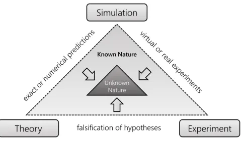
Over the last centuries the natural sciences have evolved in a process of diﬀer- entiation and specialization. The division of labor makes scientific research more eﬃcient: theoretical research focuses on forming hypotheses and analyzing results, while experimental research performs experiments and makes new observations. All this assumes that we are able to describe our subject of inquiry theoretically, and that we can devise a suitable experiment. But what if the system is too complex for theoretical treatment, too big, intricate, or costly for experimental study? With the ever-increasing computational power available to us, a third branch of science continues to thrive: simulation.

The human brain is the most complex system known. With only about 10 watts of power consumption it can perform between10¹³ and10¹⁶ synaptic operations per second [8]. Its strength lies in connecting information, processing it collectively, and finding patterns in it. However, it performs poorly when it

(10)

comes to bulk logical operations, lacking both speed and memory. Computers complement and extend our brains, and enable us to deal with amounts of information orders of magnitude larger than what all human brains together could ever process. They are the simulation tool we use to cope with systems too complex for purely theoretical and experimental study. The relationship of theory, experiment, and simulation is best illustrated by theLandau Triangle [9,10].¹

Simulation

Theory falsification of hypotheses Experiment

Unknown Nature Known Nature

Figure 1.2 –The Landau Triangle illustrates how theoretical, experimental, and computational science interact to decrease our ignorance about nature.

We have learned that in order to understand a phenomenon on one level of the structural hierarchy, we need to go one level deeper and study the components of the system and their interactions. What does that mean for simulation, which is basically a virtual experiment? It means that we need to describe the components and interactions of the system at hand as accurately as we can because their collective behavior results in the eﬀects we seek to study one hierarchical level higher. That reveals the twofold purpose of simulations: On one hand, if we understand the components of a complex system very well, we can use a simulation to predict the behavior of the system with confidence. On the other hand, by comparing the simulation of a system to reality, we can test how well we understand the components of the system.

1 Many things in physics are named after Lev Davidovich Landau, but the Landau Triangle was established by David P. Landau, professor of physics at the University of Georgia.

(11)

The Purest of Calculations 1.3 Solid state physics is a good example. Solids are collections of vast numbers

of atoms in various degrees of ordering. The properties and eﬀects on the level of the solid can only be understood by investigating how the components of the solid—electrons and nuclei—interact with each other or with external perturbations. If we have suﬃcient understanding of those components and how they interact to form a solid, and if we can translate this to a format a computer can handle, we can simulate solids and predict their properties. This is whereab initiocalculations enter the stage.

1.2 The Purest of Calculations

The Latin termab initiotranslates to “from the beginning.” This means that anab initiocalculation is an attempt to describe a systemin its entiretyusing existing theories only, ignoring all empirical knowledge about it, except the best currently known values of physical constants. An ab initiocalculation in its purest form is free of parameters and includes all theoretical models of nature down to the level of quarks. However, it is impossible (at least so far) but also unnecessary to include quantum chromodynamics or other quantum field theories in theab initiocalculation of a solid.

Fortunately, physical theories on diﬀerent scales decouple, and an entity studied by one theory can be treated as a black box by another theory one level higher in the structural hierarchy. For solids, this generally means we consider electrons and unstructured nuclei, interacting only through electromagnetism, and non-relativistic² quantum mechanics as the theoretical framework forab initio calculations.

Such a pure form ofab initiocalculation has never been seen in the wild, as a variety of simplifications and approximations on diﬀerent levels are necessary to makeab initiocalculations computationally feasible. We will focus on the most common and widespread approach for solids:ab initiodensity functional theory (DFT; see Chapter 2).

2 In some cases relativistic eﬀects have to be included even for solids, in particular when spin-orbit coupling eﬀects play a role. This is especially important for the field of spintronics.

(12)

1.3 Computational Materials Science

The technological progress of our civilization has been a sequence of increasingly advanced and impactful material technologies. It is no surprise that we label entire eras, like the Stone, Bronze, Iron, and Silicon Age, by the materials that dominated them. Today, we are beginning to understand enough about materials to move away from traditional trial-and-error materials design towards the computer-aided development of highly optimized compounds.

Computational materials science seeks to advance our abilities to interpret experiments, and to understand and predict material properties. Since material properties are relevant over many length scales, ranging from the tiniest transistors to the longest bridges, computational materials science must span many orders of magnitude (see Fig.1.3). Moreover, the goal of high-throughput materials design is obstructed by two major problems: First, predicting the most stable crystal structure of a given material is an intricate problem, and all other properties crucially depend on it. Second, the need for multi-parameter optimization, often involving quantum mechanics, is still very expensive.

Developing a unified multi-scale framework for materials design is a fascinating challenge. The development of many technologies could benefit from the computational optimization of the underlying materials, including batteries, pho- tovoltaics, hydrogen storage, medical applications, automotive and aerospace, microelectronics, and many more. With this work we contribute a computational study of two diﬀerent systems that is intended to help determine if they are suited for applications in novel material technologies.

Length scale

Electronic Atomistic Microstructural Continuum

DFT Molecular

Dynamics Physics

Continuum Equations Chemistry Materials Science Engineering

Monte Carlo

nm µm mm m

pm

Figure 1.3 –Materials modelling on different length scales is governed by different scientiﬁc disciplines and computational methods. Developing a new framework for uniﬁed multi-scale modelling remains a challenge.

(13)

The Future of Computational Science 1.4

1.4 The Future of Computational Science

Computers are the result of scientific research, and they have aided scientific research ever since. This is a positive feedback cycle resulting in an exponential growth of computational power. That observation was first popularized by Gordon Moore at Fairchild Semiconductor in 1965 and is widely known as Moore’s law[11]. It states that the complexity of integrated circuits, which is a measure of computational power, roughly doubles every 18 months. The physical limits of miniaturization are natural boundaries for the validity of Moore’s law, but inevitably new technology will increase computational power in the same way miniaturization did—and Moore’s law is likely to remain valid.

For computational science this means that raw power is not the limiting factor anymore. Instead, we will be constrained by our ability to envision and predict.

We will face increasingly data-rich problems, such as real-time streaming of volumetric data, analyzing the signals of vast sensor arrays, simulating climate and weather, predicting the consequences of natural or man-made disasters, estimating the costs and benefits of large industrial projects, distinguishing causative and correlative relations in huge datasets, and many more.

Most of these problems are ill-posed and require significant interdisciplinary eﬀort. There will soon be a need for “multi-scale intellectuals” and data scientists who try to answer questions outside of any given specialty and comfort zone.

In politics, and for society in general, simulations already have great potential to influence high-leverage decisions. Making such predictions will become increasingly simple, but it is the consequences of those predictions that matter.

Future computational science must be approached from the viewpoint of the entire ecosystem, taking all factors and resources into account. Are we ready for exaflop systems processing massive datasets on the yottabyte scale, with a power consumption of megawatts and costs of $100 million per calculation?³ We need to make sure that our algorithms are ready to exploit such expensive systems with short lifetimes.

Most important of all, we need to ensure that we learn something that is commen- surate with the investment. If we solve those problems, the continuous increase in computational power will soon allow simulations at an unprecedented scale, laying the ground for new discoveries.

3 These are actual numbers brought forward by the US National Nuclear Security Administration in 2012.

(14)

(15)

2

Density Functional Theory

Many-body systems are a fundamental challenge to theoretical physics. While quantum mechanics provides a sophisticated framework for the non-relativistic description of matter, there are only very few systems that can be solved exactly, like the hydrogen atom or the harmonic oscillator. Basically every system of three or more interacting particles escapes exact quantum mechanical treatment and needs to be caught with approximations. Those usually rely on separating the many-body wave function that describes the system as a whole into a combination of single-particle wave functions that describe either interacting particles or non-interacting particles in an eﬀective potential. This is a reasonable approach for small systems, but it does not scale very well.

Macroscopic chunks of matter contain a number of electrons on the order of the Avogadro constant^NA≈6×10²³. With four coordinates assigned to each electron (three space coordinates and one spin coordinate), the many-body wave functionΨ of such a system depends on about24×10²³ variables—it is impossible to solve the corresponding many-body Schrödinger equation.

Separating the problem into an astronomical number of single-particle wave functions is no less complex. Clearly, we need a diﬀerent approach.

(16)

2.1 Solids as Many-Body Systems

Attempting to solve the Schrödinger equation for large systems kept many luminous minds busy for the best part of the last century. A prominent result of that endeavor is density functional theory (DFT), an elegant way of treating large interacting many-body systems such as solids. Built up only from electrons and about one hundred diﬀerent kinds of atomic nuclei, solids form the vast variety of materials that surrounds us. Computational materials science makes use of the practical aspects of DFT to simulate solids, predict their properties, and motivate their use in technological applications. As we will see, three fundamental approximations to the exact quantum mechanical description of solids are necessary to reach that goal.

We start with a collection of electrons and point-like atomic nuclei in vacuum, subject to the Coulomb interaction only. The system is non-relativistic, there are no external electric or magnetic fields, and the total electric charge of the system is zero. We can then express the HamiltonianH^ˆ of this system as follows:

Hˆ=Tˆ_N+Tˆ_e+Vˆ_eN+Vˆ_ee+Vˆ_NN. (2.1) The first two terms of that sum are the kinetic energy operatorsT^ˆfor the nuclei (N) and the electrons (e), while the last three terms are the interaction potential operatorsV^ˆ for the diﬀerent combinations of particle types.

In computational materials science it is common to use atomic units to sim- plify the notation. We choose Hartree atomic units for the purposes of this exposition:¹

Hartree atomic units: m_e=e= ħ = 1

4π²0 =1. (2.2) We can now give explicit expressions for the diﬀerent terms of the Hamiltonian in (2.1). LetZidenote the charge andMi the mass of nucleusi, and letRiandrj

be the positions of nucleusi and electron j, respectively. Then the components of the Hamiltonian read

1 These units lead to formally dimensionless values. Quantities that do have a dimension in SI units are indicated by the formal unit symbol a.u. for “atomic units.”

(17)

Solids as Many-Body Systems 2.1

Tˆ_N= −1 2

X

i

1

M_i∇²_R_i, (2.3)

Tˆ_e= −1 2

X

i

∇²_r_i, (2.4)

Vˆ_eN= −X

i,j

Z_i

¯

¯R_i−r_j¯

¯

, (2.5)

Vˆ_ee= +1 2

X

i6=j

1

¯

¯r_i−r_j¯

¯

, (2.6)

Vˆ_NN= +1 2

X

i6=j

Z_iZ_j

¯

¯Ri−Rj

¯

. (2.7)

The observation that the proton mass is about 1836 times the electron mass motivates the first fundamental approximation: In typical solids, the electron dynamics happens on a scale four to five orders of magnitude faster than the dynamics of the nuclei. From the viewpoint of the electronic system the nuclei can thus be considered fixed. This is called theBorn-Oppenheimer approximation.

Applying that to the Hamiltonian in (2.1) we can drop the kinetic term^T^ˆN. Also, the interaction potential operator^V^ˆNNreduces to a constant^ENN that we will ignore in the following.

The positions of the nuclei{R₁, . . . ,R_M}, withMbeing the total number of nuclei, enter the system properties as parameters. For example, they define the adiabatic total energy surfaceE_tot(R₁, . . . ,RM). It is therefore possible to find the ideal atomic structure of a solid by minimizing its total energy with respect to these parameters. Similarly, all other system properties depend parametrically on the atomic positions. After this first approximation the Hamiltonian of a solid can be written as

Hˆ = −1 2

X

i

∇²r_i−X

i,j

Zi

¯

¯R_i−r_j¯

¯ +1

2 X

i6=j

1

¯

¯r_i−r_j¯

¯

. (2.8)

In principle, we can determine the many-body wave function of this system by solving the corresponding Schrödinger equation

i ∂

∂tΨ({ri},t)=HˆΨ({ri},t), (2.9)

(18)

where{ri}is a shorthand notation for the spatial coordinatesr1, . . . ,rm of all m electrons of the system.² Since the Hamiltonian ^H^ˆ is not explicitly time- dependent we can assume the time evolution of the wave function as

Ψ({ri},t)=Ψ({ri})e⁻^{i E t} (2.10)

and the problem reduces to the following time-independent Schrödinger equation:

Ã

−1 2

X

i

∇²_r_i−X

i,j

Z_i

¯

¯Ri−rj

¯

¯ +1

2 X

i6=j

1

¯

¯ri−rj

¯

!

Ψ({ri})=EΨ({ri}). (2.11)

The many-body wave functionΨ({r_i})is a complex, scalar function in a mul- tidimensional configuration space that is very diﬃcult to calculate in general.

Computational methods focussing on the wave function give excellent results only for small molecules. In order to reach “chemical accuracy” (that means accurate values for chemical bond lengths and cohesive energies) these methods are limited to systems with a number of chemically active electrons on the order of 10. For larger systems, wave function centered methods encounter a forbiddingexponential wallof computational and storage cost.

In fact, Walter Kohn—Nobel laureate and one of the founding fathers of modern DFT—argues that for systems with more than, say, 1000 electrons the many-body wave function is not a legitimate scientific concept anymore. Illegitimacy in this context means that such a wave function cannot be calculated with suﬃcient accuracy, nor can it be recorded for later retrieval in its entirety. This so calledvan Vleck catastropheis discussed in detail in Walter Kohn’s Nobel lecture [12].

The search for a more manageable quantity to describe large many-body systems began in 1927, just one year after Erwin Schrödinger had published his famous equation [13–16], and brought forth Thomas-Fermi density functional theory [17,18], which was later modified by Dirac [19]. Indeed, it was the first attempt to express the energy of many-body systems as afunctional of the density(hence the name), a real and scalar quantity in three-dimensional real space.

2 For the moment we do not consider the electron spin, as it has no relevance for the formal derivation of density functional theory other than enforcing a fermionic wave function that is antisymmetric under exchange of spatial coordinates.

(19)

Thomas-Fermi-Dirac Theory 2.2

2.2 Thomas-Fermi-Dirac Theory

The total energy of the homogeneous electron gas is a function of the electron density, which compeletely specifies the system. The basic idea behind Thomas- Fermi-Dirac theory (TFD) is to apply concepts of the homogeneous electron gas to inhomogeneous systems. In such systems the electron densityn(r)is a spatially varying quantity, and the components of the total energy of a system can be expressed as functionalsof it. Enrico Fermi and Llewellyn Thomas³ independently derived a functional expression for the total energy of an inhomogeneous many-body system [17,18]. Their original 1927 model did not include correlation or exchange, but Paul Dirac amended it in 1930 by adding an expression for exchange [19]:

E_TFD[n(r)]=T_e[n(r)]+E_eN[n(r)]+E_ee[n(r)]+E_x[n(r)]. (2.12) The component functionals are the kinetic energy of the electronsT_e, the interaction energy of electrons and nucleiEeN, the interaction energy of the electron density^Eee(theHartree energy), and theSlater-Dirac exchange energy^Ex. They are explicitly given by

T_e[n(r)]= 3

10(3π²)²³ Z

drn(r)⁵³, (2.13)

E_eN[n(r)]= Z

drv_ext(r)n(r), (2.14) Eee[n(r)]=1

2 Z

drdr⁰n(r)n(r⁰)

|r−r⁰| , (2.15)

E_x[n(r)]= −3 4

µ3 π

¶¹₃Z

drn(r)⁴³. (2.16)

Here, the term (2.14) includes theexternal potentialv_ext(r)created by the nuclei or an arbitrarily distributed background charge. To ensure self-consistency of the density^n(r)we need to impose the constraint of a constant total number of electrons^N:

3 Llewellyn Thomas is said to have abandoned physics later in his life, bewildered by the intricacies of quantum mechanics. He turned to computer science instead.

(20)

Z

drn(r)=N. (2.17)

This optimization problem can be solved with the method of Lagrange multipliers. The stationary solutions of the corresponding Lagrange functional with the constant Lagrange multiplierµhave to fulfill

δ δn(r)

½

ETFD[n(r)]−µ µZ

drn(r)−N

¶¾

=0, (2.18)

which leads to theThomas-Fermi equation

1

2(3π²)²³n(r)²³+ Z

dr⁰ n(r⁰)

|r−r⁰|− µ3

π

¶¹₃

n(r)¹³ =µ−v_ext(r). (2.19) Given an external potentialv_ext(r), this equation can be solved directly for the ground state densityn(r).

In general, Thomas-Fermi-Dirac theory is too inaccurate for most applications.

Crudely approximating the kinetic energy and the exchange interaction, ne- glecting electron correlation altogether, it fails to predict chemical bonding and misses essential physics. Nonetheless, it is considered as the predecessor to modern density functional theory.

From equation (2.19) we see that the electron densityn(r)uniquely determines the external potential v_ext(r) up to a constant µ. This observation inspired Pierre Hohenberg and Walter Kohn to generalize that idea in their famous Hohenberg-Kohn theorems.

2.3 The Hohenberg-Kohn Theorems

The central tenet of density functional theory is that a many-particle system is completely and exactly specified by its particle density. While Thomas-Fermi- Dirac theory hinted at it early on, it took a few more decades for that idea to mature. Eventually, it culminated in the formulation of the Hohenberg-Kohn theorems in 1964 [20].

(21)

The Hohenberg-Kohn Theorems 2.3

Theorem I

For any system of interacting particles in an external potential vext(r), the ground state particle densityⁿ0(r)uniquely determines the external potential^vext(r)up to a constant.

Given the ground state density, the external potential and thus the Hamiltonian of the system are fully determined, except for a constant energy shift. This means that also the many-body wave functions for the ground state and for all excited states are determined. Therefore, all properties of the system are completely determined by the ground state density, but how do we obtain it?

Theorem II

For any system of interacting particles in an external potentialv_ext(r), there exists a universal density functional for the total energyE_tot[n(r)]whose global minimum value is the exact ground state energyE0at the exact ground state densityⁿ0(r):^E0=^Etot[n₀(r)].

All this holds true both for systems with non-degenerate, but also with degenerate ground states, as Kohn showed in 1985 [21]. On the technical side, it should be noted that the considered densitiesn(r)must bev-representable, meaning that they are “well-behaved” (continuous, diﬀerentiable), integrate to an integer N>0, and correspond to some external potentialvext(r). Thev-representability of densities^n(r)is still a matter of ongoing research, and well-behaved densities that are notv-representable do exist [22], but these cases are rather factitious.

Fortunately, the densities of practically relevant systems are allv-representable, and this possible limitation has never been an issue in the DFT community.

While the Hohenberg-Kohn theorems are surprisingly simple to prove, their implications are tremendous: All the information that can be derived from the Hamiltonian by the solution of the Schrödinger equation is implicitly con- tained in the ground state density! The density is presented as a quantity of extraordinary richness, and the theorems point in the right direction as to the derivation of the density for arbitrary systems. However, we still lack a recipe for constructing the functionalE_tot[n(r)]to obtain the ground state densityn₀.

(22)

Theorem I states that all system properties, such as all partial energies, can be expressed as a functional of the density^n(r). Therefore the Hohenberg-Kohn (HK) total energy functional can be cast into the form

E_tot^HK[n(r)]=T[n(r)]+E_int[n(r)]+ Z

drv_ext(r)n(r), (2.20) but the exact expressions for the interacting kinetic energy functional^T^[n(r)]

and the interaction energy functionalE_int[n(r)]are unknown. At this point, Hohenberg-Kohn density functional theory is merely an exact reformulation of the many-body Schrödinger equation from the viewpoint of the particle density.

It would be of little practical use if it were not for the formalism introduced by Walter Kohn and Lu Sham in 1965 [23], which enables us to find approximate total energy functionals to replace Eq. (2.20).

2.4 The Kohn-Sham Formalism

The basic idea of the Kohn-Sham formalism is to replace the original interacting many-body system with a supplementary system of independent particles and interacting density that has the same ground state density as the original system.

This assumes the existence of such a supplementary system for each many-body system we consider—a property callednon-interacting-^v-representability. No rigorous proof has been given yet for its validity in real systems, but decades of experience suggest that it is an assumption we are safe to make [24].

For the sake of simplicity we require that the particles of the supplementary system move in alocal, spin-dependent eﬀective potentialv^σ_eff(r), so that the eﬀective single-particle Hamiltonian reads

Hˆ_eff^σ = −1

2∇²+v_eff^σ(r). (2.21) We consider a system ofN=N^↑+N^↓ electrons (the arrowsσ= ↑,↓indicate spin-up and spin-down electrons) that can be described by the above Hamilto- nian. To account for the Pauli exclusion principle we assume that in the ground state each orbitalψ^σ_i (r)of the^Nlowest energy eigenvaluesε^σ_i is occupied with one electron. The density^n(r)=n^↑(r)+n^↓(r)of the supplementary system is thus given by

(23)

The Kohn-Sham Formalism 2.4

n(r)=X

σ N^σ

X

i=1

ψ^σ_i(r)ψ^σ∗_i (r). (2.22)

The kinetic energy^Tsof the independent particles can be expressed as

T_s[{ψ^σ_i(r)}]= −1 2

X

σ N^σ

X

i=1

Z

drψ^σ∗_i (r)¡

∇²ψ^σ_i (r)¢

, (2.23)

which is an explicit functional of the orbitalsψ^σ_i(r). However, Theorem I of Section2.3tells us that it can also be viewed as a density functionalTs[n(r)]

(in fact, itmustbe one). The interaction of the electron density with itself is described by the Hartree energy

E_Hartree[n(r)]=1 2 Z

drdr⁰n(r)n(r⁰)

|r−r⁰| . (2.24) Note that the above terms for the kinetic energy and the Hartree energy do not include exchange or correlation. The brilliance of the Kohn-Sham approach is to separate out all eﬀects of exchange and correlation into an exchange-correlation functionalE_xc[n(r)], for which we can find reasonable approximations—all other terms are exactly known. We can now rewrite the Hohenberg-Kohn functional (2.20) to obtain the Kohn-Sham total energy functional:

E_tot^KS[n(r)]=T_s[n(r)]+ Z

drv_ext(r)n(r)+E_Hartree[n(r)]+E_xc[n(r)]. (2.25)

Here,^vext(r)is again the external potential of the nuclei, whose interaction en- ergyE_NNenters as a constant that can be neglected. To illustrate the significance of the exchange-correlation energy functionalE_xc[n(r)]we write it as

E_xc[n(r)]=T[n(r)]−T_s[n(r)]+E_int[n(r)]−E_Hartree[n(r)]. (2.26) This shows that the exchange-correlation term incorporates the kinetic part of the correlation energy, as well as the eﬀects of exchange and correlation of the electron-electron interaction that are not covered by the Hartree term. In that sense, the Kohn-Sham formalism can be viewed as the formal exactification of the Hartree method.

(24)

To obtain the ground state energy^E0and the ground state densityⁿ0(r)for the eﬀective Hamiltonian (2.21), which we assumed to be an equivalent description of the original interacting many-body system, we minimize the Kohn-Sham functional (2.25) subject to the constraint of orthonormal orbitals

Z

drψ^σ_i (r)ψ^σ∗_j (r)=δi,j. (2.27) Using the method of Lagrange multipliers we obtain the variational equation

δ δψ^σ∗_i (r)

½

T_s[{ψ^σ_i(r)}]+v_eff^σ(r)δn(r,σ)−εi

µZ

drψ^σ_i(r)ψ^σ∗_i (r)−1

¶¾

=0,

(2.28) whereεi is a Lagrange multiplier andv^σ_eff(r)is the eﬀective potential given by

v_eff^σ(r)=v_ext(r)+δE_Hartree[n(r)]

δn(r,σ) +δE_xc[n(r,σ)]

δn(r,σ) (2.29)

=v_ext(r)+v_Hartree(r)+v_xc^σ(r). (2.30) From Eqs. (2.22) and (2.23) we obtain

δn(r,σ)

δψ^σ∗_i (r)=ψ^σ_i(r) and (2.31) δTs[{ψ^σ_i(r)}]

δψ^σ∗_i (r) = −1

2∇²ψ^σ_i (r), (2.32)

which we insert into (2.28). This yields µ

−1

2∇²+v_eff^σ(r)

¶

ψ^σ_i(r)=εiψ^σ_i(r), (2.33) which is a Schrödinger-like single-particle equation for an eﬀective Hamiltonian that looks exactly like (2.21). This leads to the following conclusion:

(25)

The Kohn-Sham Formalism 2.4

Kohn-Sham Formalism

The ground state of any system of interacting particles in an external potential^vext(r)is equivalent to the ground state of a system of non-interacting quasiparticlesψ^σ_i (r) of energy ε^σ_i in an eﬀective Kohn-Sham potential v_KS^σ (r). The solutions of the set of Schrödinger-like single-particle Kohn- Sham equations

Hˆ_KS^σ ψ^σ_i(r)= µ

−1

2∇²+v_KS^σ (r)

¶

ψ^σ_i(r)=ε^σ_iψ^σ_i(r) (2.34) describe the ground state densityⁿ0(r)according to (2.22). The eﬀective potential^v_KS^σ ^(r)is given by

v^σ_KS(r)=v_ext(r)+v_Hartree(r)+v^σ_xc(r), (2.35) wherev_xc^σ(r)=^δ^E^xc_δ_n(r,σ)^[n(r,^σ^)] is the exchange-correlation potential, which con- tains all exchange and correlation eﬀects for which the exact analytical form is unknown. In practice one works with approximate terms for the exchange-correlation energyE_xc[n(r,σ)], whose design has become its own field of research.

It is important to note that neither the Kohn-Sham orbitalsψ^σ_i nor the energies ε^σ_i have any physical meaning. The only connection to the real, physical world is through Eq. (2.22) and the fact that the highest occupied stateε^σ_i , relative to the vacuum, equals the first ionization energy of the system. Other than that, theε^σ_i are just Lagrange multipliers and theψ^σ_i are quasiparticles that by construction reproduce the ground state densityn₀(r)of the original system. It is the ground state density that connects these quantities, which have a well-defined meaning only within the Kohn-Sham theory, to all other physical properties of the system.

Unfortunately, the detour via the Kohn-Sham orbitals is necessary to obtain the ground state density. It is entirely possible that there is a practical way to derive the density directly from the Hamiltonian, but it has not been found yet.

Nonetheless, the Kohn-Sham formalism and the Hohenberg-Kohn theorems provide an exact, density-centered reformulation of the interacting many-body problem with profound consequences.

(26)

First, the Hohenberg-Kohn formulation of DFT replaces the virtually unsolvable problem of the many-body Schrödinger equation with the minimization of a density functional of the energy. Second, the Kohn-Sham formalism shows that we can minimize that functional by solving a set of independent single-particle equations involving an eﬀective potential. That potential in turn is structured such that all terms whose exact analytical form is unknown are separated out into a local or nearly local exchange-correlation potential for which we can find practical approximations. It is this reformulation of the original problem on many levels that makes the numerical treatment of interacting many-body systems feasible.

2.5 Exchange-Correlation Functionals

The pivotal entity of density functional theory is the exchange-correlation func- tionalE_xc[n(r)], whose existence is guaranteed by the Hohenberg-Kohn theorems. Any DFT calculation is only as good as the approximation it uses for that functional. The growing success of DFT over the last decades was nurtured by rapidly advancing computational prowess and the development of suﬃciently accurate and versatile approximations to the exact exchange-correlation functional. While the Born-Oppenheimer approximation was the first fundamental approximation to the exact solid state Hamiltonian on our way towards a numerical treatment, the approximation of the exchange-correlation energy functional in DFT is the second one.

Nowadays, a vast zoo of functionals is available for all kinds of applications and classes of materials. Each functional has its idiosyncrasies, and some are applicable to a wide range of materials, while others should only be used for the special cases in which they excel. Exchange-correlation functionals can be classified by their locality properties, the amount and type of information they take into account, their degree of empiricism, and the constraints they satisfy.

There are two basic approaches to constructing an exchange-correlation functional:nonempirical constraint satisfactionandsemiempirical fitting [25]. The first approach tries to construct parameter-free (except for fundamental constants) functionals that conform to formal properties of the exact exchange- correlation energy, such as scaling laws and asymptotic behavior. The second approach tends to disregard those formal constraints and fits the functionals to large empirical datasets gathered from experiments or accurate many-body calculations.

(27)

Exchange-Correlation Functionals 2.5 Nonempirical constraint satisfaction is a scientifically sound, prescriptive way

to construct a hierarchy of exchange-correlation functionals with systematically increasing accuracy. The resulting functionals are universal by design and can be applied to a wide range of materials. In contrast, semiempirical functionals are descriptive. They typically involve many empirical parameters and produce accurate results only for systems not too diﬀerent from the ones used for fitting the functionals. Many such functionals violate the formal constraints imposed by the exact exchange-correlation energy and fail to correctly describe even the one case where they could be exact: the homogeneous electron gas.

Semiempirical functionals are especially popular in quantum chemistry, which deals with molecular, localized systems, while solid state physics deals with extended, periodic systems, which require more universal, nonempirical functionals. This has caused many a controversy over which type of functional should be favored. In the solid state DFT community, philosophical and practical preference is given to nonempirical functionals.

John Perdew illustrated the classification of nonempirical functionals with his Jacob’s Ladder⁴ of exchange-correlation functionals [26] that leads from the inaccurate “Hartree world” to the “heaven of chemical accuracy”⁵ (see Fig.2.1).

Users of DFT can ascend or descend along its rungs depending on their accuracy needs and the computational price they are willing to pay.

Climbing the ladder, the accuracy of the functionals increases with each rung.

So does the computational cost and the conceptual complexity involved. Just like Russian matryoshka dolls, the functionals on each rung encompass the functionals on all lower rungs. By taking more information into account with each rung, more formal constraints imposed by the exact exchange-correlation energy can be satisfied. This produces a cadence of nonempirical functionals with systematically increasing complexity, accuracy and nonlocality.

The simplest approximation (the first rung) is to assume that the eﬀects of exchange and correlation are purely local and can be described by the exchange- correlation energy of a homogeneous electron gas with a specific density. This is called thelocal spin density approximation(LSDA) [23]:

E_xc^LSDA[n(r,σ)]= Z

drn(r,σ)²^hom_xc ¡

n(r,σ)¢

. (2.36)

4 In Christian mythology, Jacob betrayed his older brother Esau of his birthright. During his escape, Jacob dreams of a ladder from earth to heaven, on which angels are ascending and descending.

5 Chemical accuracy means that we can accurately describe the rates of chemical reactions. This translates to an energy error on the order of∆E/1^kcal_mol=0.0434 eV.

(28)

Hartree World LSDA

GGA meta-GGA

hybrid fully non-local Heaven of Chemical Accuracy

local spin density approximation generalized gradient approximation meta-generalized gradient approximation exact exchange and compatible correlation exact exchange and exact partial correlation

density n(r) density gradient n(r) kinetic energy density τ(r) occupied ψ_i(r) unoccupied ψ_i(r)

Figure 2.1 –(Adapted from [25]) The Jacob's Ladder of exchange-correlation functional approximations (after John Perdew). With each rung, additional ingredients (given on the left) are taken into account, which leads to an increase in accuracy, complexity, and computational cost.

Here,²^hom_xc ¡

n(r,σ)¢

is the exchange-correlation energy per particle of a homogeneous electron gas of densityn(r,σ). The spin quantization axis is assumed to be the same over the whole space.

LSDA assumes that a solid can locally be described by a homogeneous electron gas, which turns out to be a remarkably good approximation in many cases, even for solids with rapid electron density variations. This is because LSDA inherits the exact properties of the homogeneous electron gas and satisfies many of the general constraints on the exchange-correlation energy. Owing to its reasonable description of solids without long-range correlation eﬀects, LSDA is still a widely used functional in solid state DFT. However, although it produces reasonably accurate bond lengths, it is less useful for molecular systems as it greatly overestimates binding energies.

This flaw can be mitigated by taking not only the local density, but also the local density gradient into account (second rung of the ladder). This requires knowledge of the density in a single point of space and in an infinitesimal re-

(29)

Exchange-Correlation Functionals 2.5 gion around that point, resulting in a class of semilocal functionals collectively

calledgeneralized gradient approximation(GGA) [27–29]. All GGA exchange- correlation energy functionals have the general form

E_xc^GGA[n(r,σ)]= Z

drn(r)²^GGA_xc ¡

n(r,σ),∇n(r,σ)¢

, (2.37)

where the exchange-correlation energy per particle²^GGA_xc depends on the spin- resolved density and density gradient. Naively one would think that for slowly varying densities the simple second-order gradient expansion (GE2),

E^GE2_xc [n_↑,n_↓]= Z

dr

"

n²^hom_xc (n_↑,n_↓)+X

σ,σ⁰

C_xc^σσ⁰(n_↑,n_↓)∇n_σ· ∇n_σ0

n_σ^2/3n^2/3_σ₀

#

, (2.38)

is an improvement over LSDA. However, that expression violates an exact sum rule and performs worse than LSDA for many realistic systems [30]. The in- adequacy of GE2 demonstrates precisely why it is so important to satisfy the constraints imposed by the exact exchange-correlation energy. The widely used and recommended GGA of John Perdew, Kieron Burke, and Matthias Ernzerhof (PBE) [27] is entirely nonempirical and honors all constraints that can be satisfied on the second rung of the ladder. It was used for all calculations presented in this work.

Meta-GGAs form the third rung of the ladder and take the kinetic energy densitiesτσ(r)of all occupied Kohn-Sham orbitals into account, where

τσ(r)=1 2

occ.

X

i

|∇ψ^σ_i (r)|². (2.39)

The kinetic energy densitiesτ_σ(r)are implicit functionals of the density and allow for the satisfaction of more constraints than the Laplacians∇²n_σ(r), which they contain in the limit of slowly varying density.

So far, there is only one nonempirical meta-GGA, developed by Tao, Perdew, Staroverov, and Scuseria (TPSS) [31], which is of the form

E_xc^TPSS[n(r,σ)]= Z

drn(r)²^TPSS_xc ¡

n(r,σ),∇n(r,σ),τ_σ(r)¢

. (2.40)

(30)

TPSS does not satisfy all possible rung-three constraints, but it easily keeps pace with semiempirical functionals and greatly improves on PBE when it comes to molecular atomization energies and solid surface energies (see [25] and references therein).

On the fourth rung of the ladder, the exact exchange energy density²^σ_x(r), which is a fully non-local functional of the Kohn-Sham orbitalsψ^σ_i(r), is added as an ingredient. Here we find hybrid functionals that mix some exact exchange into meta-GGA or GGA exchange-correlation [32], like

E_xc^hybrid=E_xc^(meta−)GGA+a¡

E_x^exact−E_x^(meta−)GGA¢

, (2.41)

where 0≤a ≤1with an optimal choice of a =1/4. Other rung-four functionals are hyper-GGAs, which use exact exchange and compatible correlation constructed from meta-GGA ingredients [26]. Compatible means that the correlation part must be fully non-local at least in the occupied Kohn-Sham orbitals, like the exact exchange part. Popular semiempirical functionals like B3LYP [28,29] are found on this level, while comparable nonempirical functionals are in development [33].

The fifth and final rung comprises functionals that combine exact exchange with a partially summated perturbation expansion of the correlation [26]. They are fully non-local functionals of the occupied as well as the unoccupied Kohn-Sham orbitals. On this level, there are no functionals for general use yet.

2.6 Self-Consistency

Choosing a suitable approximation to the exchange-correlation functional is not enough to set up and solve the Kohn-Sham equations. In order to construct the eﬀective potentialv^σ_KS(r)of (2.35) we need the densityn(r), and to obtain the density we need to solve the Kohn-Sham equations. Only an iterative approach can break this circle and reach approximate self-consistency of the density (or the eﬀective potential, which is equivalent).

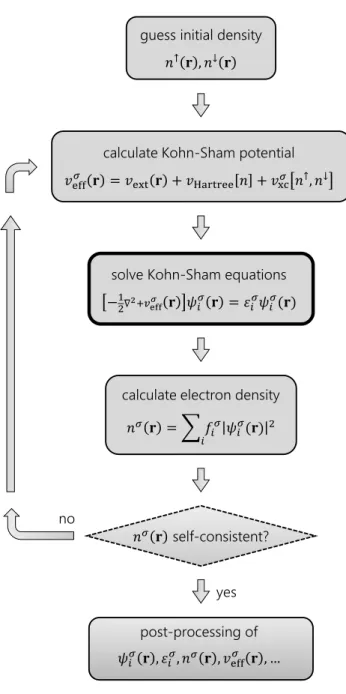
This approach is called theself-consistent field cycle(SCF cycle) and is illustrated in Fig.2.2. We start with an initial estimate of the input density, which is typically a superposition of the atomic densities of the system. From that we construct the eﬀective potential and set up the Kohn-Sham equations. What follows is the computationally most expensive step of solving the Kohn-Sham equations

(31)

Self-Consistency 2.6 for a given basis set (see Section2.7) to obtain the Kohn-Sham orbitals and

energies. A new output density can then be calculated from those orbitals according to (2.22). That output density is necessarily diﬀerent from any estimated, non-self-consistent input density.

guess initial density 𝑛^↑ 𝐫 , 𝑛^↓ 𝐫

calculate Kohn-Sham potential 𝑣_eff^𝜎 𝐫 = 𝑣_ext 𝐫 + 𝑣_Hartree 𝑛 + 𝑣_xc^𝜎 𝑛^↑, 𝑛^↓

solve Kohn-Sham equations

−¹_2∇²+𝑣_eff^𝜎 𝐫 𝜓_𝑖^𝜎 𝐫 = 𝜀_𝑖^𝜎𝜓_𝑖^𝜎(𝐫)

calculate electron density 𝑛^𝜎 𝐫 =

𝑖𝑓_𝑖^𝜎 𝜓_𝑖^𝜎(𝐫)²

𝑛^𝜎 𝐫 self-consistent?

no

yes post-processing of 𝜓_𝑖^𝜎 𝐫 , 𝜀_𝑖^𝜎, 𝑛^𝜎 𝐫 , 𝑣_eff^𝜎 𝐫 , …

Figure 2.2 –Schematic prescription for an iterative, self-consistent solution of the Kohn- Sham equations.

(32)

The key to reaching self-consistency fast is to mix the output density with the input density of the same iteration in a clever way to generate the input density for the next iteration. This problem is more complicated than it seems. Simply using the output density as the new input density fails badly in many ways,⁶and linear schemes to update the density (linear mixing), such as

nⁱⁿ_i+1=nⁱⁿ_i +α¡

n^out_i −nⁱⁿ_i ¢

, (2.42)

wherei is the iteration index and0≤α≤1is the mixing factor, are very ineﬃ- cient and not practical.

Methods involving the Jacobian or Hessian matrix prove to be more eﬃcient than linear mixing. The family ofBroyden mixingmethods [36–41] take not only numerical details, but also algorithmic complexity into account, and update the inverse Jacobian successively with each iteration. Their eﬃciency has lead to the widespread use of Broyden-type mixing in contemporary Kohn-Sham solvers.

Even more eﬃcient and versatile, but also more complex mixing schemes are available in most DFT implementations today.

For real systems it is impossible to find the exact self-consistent density with numerical methods, but we can come arbitrarily close. Given an adequate mixing scheme, the input and output densities of the SCF cycle will diﬀer less and less with each iteration, until finally a judiciously chosen convergence criterion is reached. Thedensity distance^dnis such a criterion:

d_n= 1 Ωcell

Z

Ωcell

dr¡

n^out(r)−nⁱⁿ(r)¢2

≤d_n^conv. (2.43) Here,Ωcellis the real-space unit cell volume, and convergence is reached when at the end of an SCF iteration the density distance is smaller thand_n^conv. In a similar fashion, the diﬀerence of input and output values of many quantities derivable from the Kohn-Sham Hamiltonian can serve as a convergence criterion.

Examples are thecharge distancedQ = −edn(eis the positive elementary charge) or the total energyEtotper unit cell.

In practice, the ground state densityn₀(r)itself is seldom the quantity of interest.

Most DFT calculations involve finding the ground state density as the initial step, whose output is then processed to obtain other properties of the system, such as its electronic, mechanical, or optical properties. Post-processing a converged

6 The reason for this is the behavior of the pre-self-consistent Kohn-Sham density near the minimum of the