Community composition of epipelagic zooplankton in the Eurasian Basin 2017 determined by ZooScan image analysis
von Julian Koplin
geboren am 05.07.1994
Bachelorarbeit
im Studiengang Bachelor of Science Biologie der Universität Hamburg
25.04.2020
Erstgutachter: Dr. Jens Floeter
Table of Contents
1 Introduction ... 1
2 Material and Methods ... 6
2.1 Sampling ... 6
2.2 Sample analysis ... 8
2.3 ZooScan image analysis ... 9
2.4 Abundance, Biovolume and Biomass ... 10
2.5 Statistical analysis ... 13
3 Results ... 14
3.1 Description of the taxa, community composition and taxa abundance ... 14
3.2 Copepods ... 18
3.3 Selected copepod taxa ... 20
3.3.1 Calanus finmarchicus/glacialis ... 20
3.3.2 Calanus hyperboreus ... 21
3.3.3 Metridia longa ... 22
3.4 Non-copepod taxa ... 23
3.5 Biovolume and Biomass ... 25
3.6 Composition of size-fractions ... 29
3.7 Comparison of Abundance, Biovolume and Biomass ... 32
3.8 Comparison of ZooScan-based biomass and dry weight biomass ... 33
4 Discussion ... 36
5 Literature ... 44
6 Appendix ... 52
7 Acknowledgements ... 57
Declaration of academic honesty ... 57
Table of Figures
Figure 1: Bathymetric map of the Arctic Ocean, the red arrows showing general circulation and the bigger arrows the importance of riverine inflow. From Michel et al. (2012), adapted from Carmack (2000) and Jakobsson et al. (2004, 2008). ... 3 Figure 2: Overview of the RMT stations during the Polarstern expedition PS106.2 ... 6 Figure 3: Water masses of upper 400 m at all station, hydrographic information by A.
Nikolopoulos (unpublished data) ... 8 Figure 4: Results of cluster analysis of 15 stations (samples), analysis based on Bray Curtis similarity. With cluster numbers 1 and 2. ... 14 Figure 5: Taxonomic composition at all stations. Abundances (left panel) and relative
abundances (right panel). Copepoda with a contribution < 4% are grouped as “Other
Copepoda” and non-copepod taxa with contribution <1% are grouped as “Other Taxa. ... 17 Figure 6: Species composition of copepods at all stations. Abundances (left panel) and
relative abundances (right panel). Copepods with contribution <4% were grouped as “Other Copepoda”, Calanoida with contribution <3% were grouped as “Other Calanoida”. ... 20 Figure 7: Developmental stage composition of Calanus finmarchicus/glacialis at all stations.
Abundances (left panel) and relative abundances (right panel). ... 21 Figure 8: Stage composition of Calanus hyperboreus at all stations. Abundances (left panel) and relative abundances (right panel). ... 22 Figure 9: Stage composition of Metridia longa at all stations. Abundances (left panel) and contribution (right panel). ... 23 Figure 10: Species composition of non-copepods at all stations. Abundances (left panel) and relative abundance (right panel). Taxa with contribution <0.05% were grouped as “Other Taxa” ... 24 Figure 11: Biovolume in mm3 m-3 at all stations (left panel) and biovolume contribution at all stations (right panel). Split in size-fractions. ... 26
Figure 12: Relationship between ZooScan-based biovolume and biomass converted from the biovolume, with linear trend-line. There is a significant positive relationship. Linear
regression: y = 11.74x + 46.574 R2 = 0.81, p < 0.001) ... 26 Figure 13: Total biomass (mg m-3) of all 15 stations, split by cluster. Median values marked as red crosses (x). ... 28 Figure 14: Biomass in mg m-3 at all stations (left panel) and biomass contribution at all
stations (right panel). Split in size-fractions. ... 28 Figure 15: Total biomass in mg m-3 for all size-fractions (left panel) and biomass contribution for all size-fractions in % (right panel). ... 29 Figure 16: Total biomass contribution (%) of Copepoda taxa, split in size-fractions ... 31 Figure 17: Relationship between biomass and abundance, with linear trend-line. There is a significant positive relationship. Linear regression: y = 8.0109x – 13.072 R2 = 0.89, p <
0.001) ... 32 Figure 18: Relationship between biovolume and abundance, with linear trend-line. There is a significant positive relationship. Linear regression: y = 0.5288x – 23.282 R2 = 0.66, (p<0.001) ... 32 Figure 19: Relationship between ZooScan-based biomass and dry weight measured biomass, with linear trend-line. Blue line indicates 1:1 relationship. There is a significant positive relationship. Linear regression: y = 0.3714x + 1.3301 (R2 = 0.573, p =0.004) ... 33 Figure 20: Accumulated biomass of all stations, split in size-fractions ... 35 Figure 21: Exemplary relationship between ZooScan-based biomass and dry weight measured biomass with trendline, for the size-fractions 500-1000 µm (gray), 1000-2000 µm (yellow) and 2000-4000 µm (blue). ... 35 Figures in Appendix
Figure A. 1: Confusion matrix from EcoTaxa, diagonal contains the recall rate, darker blue indicates a higher rate. For all categories see Tab. A.3. ... 55 Figure A. 2: Confusion matrix from EcoTaxa, diagonal contains the precision rate, darker blue indicates a higher rate. For all categories see Tab. A.3. ... 55
List of Tables
Table 1: Summary of RMT hauls conducted during PS106/2 ... 7
Table 2: Reg. and corr. parameters obtained from Lehette and Hernandez-Leon (2009) ... 12
Table 3: Total number of taxa and combined abundance of all taxa at the sampling sites. Split in size-fractions. ... 15
Table 4: Abundance of all Copepods at the sampling sites. Split in size-fractions. ... 16
Table 5: Abundance of all taxa within different size-fractions, both Clusters and overall in ind. m-3, median, 25%, 75% quantile (Q.) and average with standard deviation. ... 16
Table 6: Shannon-Wiener Index and Evenness of all stations ... 17
Table 7: Abundance of copepods at all stations, median, quartile (Q.) and average (Avr.) with standard deviation (SD) of all taxa in ind. m-3, ... 18
Table 8: Total relative abundance of copepods at each station in % ... 19
Table 9: Abundance of non-copepods at all stations, median, quartile (Q.) and average (Avr.) with standard deviation (SD) of all taxa in ind. m-3, ... 25
Table 10: Contribution of size-fractions for zooplankton biomass and biovolume in % ... 27
Table 11: Contribution over all stations for zooplankton biomass and biovolume in % ... 27
Table 12: Total biomass of taxa, median, quartile (Q.) and average (Avr.) with standard deviation (SD) of all taxa in mg m-3, split in size-fractions. ... 30
Table 13: Total biomass contribution of taxa in %, split in size-fractions. ... 30
Table 14: Total biomass of Copepoda (mg m-3), split in size-fractions. ... 31
Table 15: Total biomass contribution of Copepods (%), split in size-fractions. ... 31 Table 16: Total relative contribution of biomass and abundance in %, split in size-fractions. 33
Tables in Appendix
Table A. 1: Taxonomic composition and abundance of mesozooplankton across the Barents Sea shelf slope and Nansen Basin for the Atlantic regime Cluster (AR) ... 52 Table A. 2: Taxonomic composition and abundance of mesozooplankton across the Barents Sea shelf slope and Nansen Basin for the polar regime Cluster (PR) ... 53 Table A. 3: Summary of statistical evaluation (n = sample size, W = Wilcoxon statistical criterion, p-value) ... 54 Table A. 4: All categories of the learning set in EcoTaxa ... 56
Abbreviations
AR Atlantic regime Avr Average
AW Atlantic Water
AWI Alfred Wegener Institute C. Calanus
H Diversity index of Shannon Wiener MAW Modified Atlantic Water
PR Polar regime
PSW Polar Surface Water Q. Quartile
RMT Rectangular Midwater Trawl SD Standard deviation
wPSW warm Polar Surface Water
Summary
The Arctic Ocean is especially vulnerable to the impacts of climate change. Warmer ocean temperatures and reduced sea ice coverage lead to a poleward shift of communities in the Arctic Ocean. This process, termed borealization, is considerably changing Arctic marine food web structure with implications for ecosystems dynamics and functioning. Zooplankton is a good indicator of climate change in the marine environment and helps understand what role aberrations in the water mass circulations could play for ecosystem functioning.
To better understand how the communities adapt to the changing environment and what the potential impacts, such as borealization, could mean for the arctic habitats, monitoring the community composition on a regular basis is crucial. Traditional taxonomical analyses are time consuming while the semi-automatic image analysis using ZooScan was developed to reduce time.
This study aims to provide further information on the composition of epipelagic zooplankton communities in the Arctic Ocean determined by ZooScan image analysis and to verify whether there is a biogeographical and hydrographical pattern on the shelf and slope of the Barents Sea and in the Nansen Basin. Additionally, this study tried to confirm whether the taxonomy-based optical method ZooScan leads to similar results as dry-weight measured biomass data in term of size distribution and total biomass in different size fractions.
The expedition PS 106.2 with the research vessel Polarstern provided an opportunity to sample the epipelagic zooplankton community from the shelf of the Barents Sea into the Nansen Basin proper, crossing a gradient of decreasing influence of Atlantic Water (AW).
This study confirmed the hypothesis that there was a biogeographical and more importantly hydrographical pattern of mesozooplankton community structure in the study area of PS106.
The basin domain is characterized by two basic water masses. The Atlantic regime (AR) with near-surface Atlantic Water (AW) and the polar regime (PR) with AW at a greater depth, overlain with polar surface water and intermediate water. Biomass and abundance were highest along stations in the AR and lowest at stations in the PR. Smaller fractions with high abundances dominated the AR and bigger fractions the PR respectively. In warming Arctic Ocean, growing AW influences can therefore have consequences for the ecosystem structure
Calanus glacialis and the boreal species Calanus finmarchicus were found dominant in the AR. In contrast Calanus hyperboreus and Metridia longa dominated the PR. This study showed that a more traditional method for calculating biomass such as a dry weight measurement leads to similar relative proportions as ZooScan-based biomass. This would allow for a more rapid taxonomic analysis and biomass calculation of the vast number of samples. However, a correct parametrization of the conversion from 2-dimensional objects on ZooScan pictures to dry mass is critical for an accurate determination of dry weight. Finally, there was a link between high biomasses and high abundances, which could enable faster predictions based on biomass alone in well-studied ecosystems.
Zusammenfassung
Der Arktische Ozean ist besonders anfällig für die Auswirkungen des Klimawandels.
Wärmere Meerestemperaturen und eine verringerte Meereisbedeckung führen zu einer polwärts Verschiebung von Gemeinschaften im arktischen Ozean. Dieser als Borealisierung bezeichnete Prozess verändert die Struktur des arktischen marinen Nahrungsnetzes erheblich und hat Auswirkungen auf die Dynamik und Funktionsweise der Ökosysteme. Zooplankton ist ein guter Indikator für Klimaveränderungen in der Meeresumwelt und hilft zu verstehen, welche Rolle Veränderungen der Wassermassenzirkulation für das Funktionieren arktischer Ökosysteme spielen könnten.
Um besser zu verstehen, wie sich die arktischen Gemeinschaften an das sich ändernde Umfeld anpassen und welche potenziellen Auswirkungen Veränderungen wie die Borealisierung auf die arktischen Lebensräume haben könnten, ist eine regelmäßige Erfassung der
Zusammensetzung der Zooplanktongemeinschaften von entscheidender Bedeutung.
Herkömmliche taxonomische Analysen sind zeitaufwändig, jedoch wurde mit der
halbautomatischen Bildanalyse mit dem ZooScan ein Verfahren entwickelt, das schneller zu Ergebnissen führt.
Diese Studie soll weitere Informationen über die Zusammensetzung der epipelagischen Zooplanktongemeinschaften im Arktischen Ozean liefern, die durch die ZooScan-Bildanalyse ermittelt wurden. Außerdem sollte überprüft werden, ob im Schelf und am Hang der
Barentssee sowie im Nansen-Becken ein biogeografisches und hydrographisches Muster vorliegt. Darüber hinaus wurde in dieser Studie versucht zu bestätigen, ob die
taxonomiebasierte optische Methode ZooScan zu ähnlichen Ergebnissen führt wie die gemessenen Trockenmasse-Biomassedaten hinsichtlich Größenverteilung und
Gesamtbiomasse.
Die Expedition PS 106.2 mit dem Forschungsschiff Polarstern bot die Gelegenheit, die epipelagische Zooplanktongemeinschaft vom Schelf der Barentssee bis in das eigentliche Nansen-Becken zu untersuchen und dabei einen Gradienten mit abnehmendem Einfluss von Atlantischen Wasser (AW) zu überqueren.
Diese Studie bestätigte die Hypothese, dass es im Untersuchungsgebiet von PS106 ein biogeografisches und vor allem hydrographisches Muster der Mesozooplanktongemeinschaft gibt. Die Beckendomäne ist gekennzeichnet durch zwei Grundwassermassen. Das atlantische Regime (AR) mit oberflächennahmen AW und das polare Regime (PR) mit AW in größerer
Kleinere Fraktionen mit hoher Abundanz dominierten das atlantische Regime und größere Fraktionen das PR. Wachsende AW-Einflüsse könnten daher Konsequenzen für die
Ökosystemstruktur und die Nachhaltigkeit von Meeresressourcen bedeuten. Calanus glacialis und die boreale Art Calanus finmarchicus waren im AR dominant während Calanus
hyperboreus und Metridia longa das PR dominierten. Es wurde gezeigt, dass eine
traditionellere Methode zur Berechnung von Biomasse, wie Trockengewichtsmessung, zu ähnlichen relativen Ergebnissen führt wie Biomassebestimmung durch ZooScan, was eine schnellere taxonomische Analyse und Biomasseberechnung der großen Anzahl von Proben ermöglichen würde. Allerdings zeigte sich, dass eine korrekte Parametrisierung der
Konversion von flächenbasierten ZooScan-Aufnahmen auf die Trockenmasse kritisch für eine akkurate Ableitung der Trockenmasse ist. Schließlich bestand ein Zusammenhang zwischen hoher Biomasse und hoher Abundanzen, was schnellere Vorhersagen auf der Grundlage von Biomasse allein in gut untersuchten Ökosystemen ermöglichen könnte.
1 Introduction
In most oceans, zooplankton constitutes a key link in the food chain between primary producers and higher trophic levels. In the Arctic Ocean, they represent the most important prey of various higher trophic levels such as capelin and polar cod (Wassmann et al 2006).
Changes in zooplankton communities could therefore have far-reaching consequences for the food web and commercial fishing.
Because of their low swimming ability and short life cycle (Wassmann et al. 2006)
zooplankton respond easily to variability in the physical environment, such as temperature, algal biomass, and changes in oceanic current systems (Hays et al 2015). This makes them a good indicator of climate change in the marine environment and helps understand what role changes in the water mass circulations could play (Hays et al. 2005, Blachowiak 2008).
Warmer ocean temperatures and reduced sea ice coverage lead to a poleward shift of communities in the Arctic Ocean (Fossheim et al. 2015). This process has been termed
“borealization” and is considerably changing Arctic marine food web structure with implications for ecosystem dynamics and functioning (Kortsch 2015).
Monitoring the community composition on a regular basis will help to better understand how the communities adapt to the changing environment and what the potential impacts, such as borealization, could mean for the arctic habitats.
The Arctic Ocean is the smallest ocean region, consisting of a deep basin surrounded by shelf seas with an average depth of 1050 meters (Pidwirny 2006), almost completely surrounded by land. The exchange with the Atlantic and Pacific oceans is limited. The shallow continental shelves surrounding the deep central basin have an average depth of 100 m (Jakobsson et al.
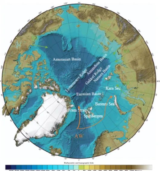
2003). These coastal areas are seasonal ice zones that receive 10% of the global river runoff and can sustain high productivity (Rudels et al. 1994, Schauer et al. 1997, Figure 1). The deep central basins on the other hand have been perennially ice-covered and are considered to be less productive (Sakshaug et al. 2004).
The central Arctic Ocean is subdivided into two basins by the Lomonosov Ridge: the
Amerasian and Eurasian Basins (Jakobsson et al. 2003). The Eurasian Basin is subdivided in
The dominant hydrographic feature of the Eurasian Basin is the Atlantic water (AW) inflow from the Nordic Seas. The Nansen Basin is affected by the Fram Strait inflow branch of the AW, as well as typical shelf water masses from the Barents Sea shelf. These two branches are interacting with each other and when meeting the two branches create intrusive layers, not only north of the Kara Sea between the main Barents Sea branch inflow but also north of Franz Josef Land, where a smaller fraction of the Barents Sea inflow enters the Nansen Basin (Rudels et al. 2013). Within the basin domain two basic water mass assemblies are observed, the difference between them being the absence or presence of Modified Atlantic Water (termed polar water by Bluhm et al. 2015) sandwiched between Polar Surface Water (termed Arctic Surface Water Bluhm et al. 2015) above and the AW below (Bluhm et al. 2015). The AW core is located rather shallow (100-200 m), however the whole Atlantic layer extends down to 750 m depth in the research area of this study (Nikolopoulos et al. 2018).
The Barents Sea is a shelf sea with depths ranging from 50 m at the shallow banks to 500 m at the deeper points (Sundfjord et al. 2007). The northern regions of the Barents Sea are
seasonally covered by sea ice, with a maximum and minimum ice cover in April and
September (Vinje and Kvambekk 1991). The Barents Sea is influenced by the confluence and mixing of different water masses. Warm, salty and nutrient-rich AW enters the Barents Sea from the southwest, overlain by Arctic Water that mixes with fresh meltwater (Sundfjord et al. 2007, Loeng 1991). The Barents Sea alone lost 50% of the annual ice cover between 1998 and 2009 (Årthun et al. 2012). Among other things, the vertical stratification of the waters has changed, which leads to a potentially higher penetration of vertical thermal convection into the warm, saline Atlantic layer. More heat and salt are consumed, leading to heating and salinification of the overlying Artic water layer. In winter this leads to an additional loss of sea ice (Aksenov and Ivanov 2018).
Figure 1: Bathymetric map of the Arctic Ocean, the orange arrows showing Atlantic water (AW) inflow and the green arrows the importance of riverine inflow (RR). Underlying map was obtained from NOAA, the National Oceanic and Atmospheric Administration (https://www.ngdc.noaa.gov/mgg/bathymetry/arctic/currentmap.html)
In terms of zooplankton biomass, the region is clearly dominated by Arctic copepods, predominantly Calanus glacialis Jaschnov, 1955, Calanus finmarchicus (Gunnerus 1770), Calanus hyperboreus Krøyer 1838 and Metridia longa (Lubbock 1854) (Falk-Petersen et al.
2009, Ksobokova 2009, David et al. 2015). C. hyperboreus and C. glacialis are considered Arctic endemic species and associated with cold Arctic water.
However, growing influence of AW in the Arctic could lead to a shift from the larger Arctic Calanus species toward the smaller Atlantic/boreal C. finmarchicus, therefore changing the community structure (Kortsch 2015). All the species have distinct life cycles, with C.
finmarchicus having a one-year lifecycle in the Barents Sea, spawning in spring with the RR
RR RR
AW
Long time-series to monitor plankton and identify future changes in marine ecosystems are crucial (Hays et al. 2015). Traditional taxonomical analyses are not only time consuming, but greatly dependent on taxonomic expertise and hence expensive. This can lead to fragmented information that may be difficult to understand, because only a limited number of samples can be processed (Grosjean et al. 2004).
With new technology, such as the ZooScan, multiple organisms in a sample can be
determined relatively quickly, and automatic prediction based on deep-learning algorithms saves time with identification (Benfield 2007). Unlike methods using DNA barcoding, the organisms do not have to be destroyed and can be kept for further investigations (Gorsky et al. 2010). Scanned organisms with attached metadata can also be shared between scientists for further analysis. Several scientists can work simultaneously on identifying organisms and correct previous identification if necessary. This could drastically reduce the number of identification mistakes. In addition, attached metadata can be used to carry out various calculations, such as determining abundances or biovolumes.
The goal of this bachelor thesis is to provide further information on the composition of epipelagic zooplankton communities in the Arctic Ocean determined by ZooScan image analysis (Grosjean et al. 2004) to verify whether there is a biogeographical and
hydrographical pattern on the shelf and slope of the Barents Sea and in the Nansen Basin.
From the abundances determined with ZooScan, the corresponding biomass will be calculated and compared with the directly measured dry-weight biomass of the master thesis “Trophic structure and biomass of high Arctic zooplankton in the Eurasian Basin in 2017” by Nadezhda Zakharova (2019). Thereby it can be examined whether a taxonomic method such as ZooScan analysis leads to similar results as dry-weight measured biomass data. The study of
zooplankton biomass by Zakharova (2019) showed unexpected results. The zooplankton biomass was highest on the shelf, but significantly lower on the slope than in the deep-sea- basin. Furthermore, no statistical differences in total biomass in relation of the influence of AW was confirmed, however smaller size fractions dominated stations more exposed to AW.
The detailed taxonomic results regarding abundances and biomasses, acquired by the ZooScan method, are examined further to investigate how biomass can act as proxy for abundance and community composition to further speed up sampling analyses.
The following hypotheses were therefore examined in the present study:
The variability of the zooplankton community mirrors biogeographical and hydrographical patterns along the Barents Sea shelf and into the Nansen Basin.
• A taxonomy-based optical method such as ZooScan analysis leads to similar results as dry-weight measured biomass data in terms of size distribution and total biomass.
• Biomass data can act as proxy for abundance in a taxonomically well-described ecosystem
2 Material and Methods
2.1 Sampling
The expedition PS 106/2 with the research vessel Polarstern provided an opportunity to sample the epipelagic zooplankton community from the shelf of the Barents Sea into the Nansen Basin proper, crossing a gradient of decreasing influence of Atlantic Water (AW).
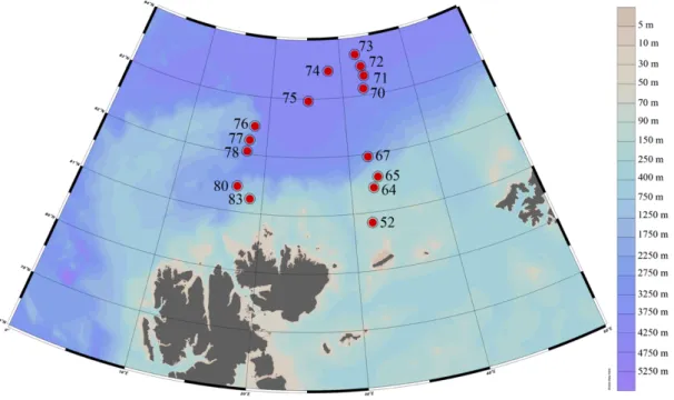
From June 29, 2017, to July 13, 2017 the pelagic community was sampled with double- oblique hauls over a depth range of 0-100 m with a Rectangular Midwater Trawl (RMT). A detailed description of the sampling procedure during the cruise PS106.2 is available at Flores et al. (2018). Fifteen stations were sampled, of these, stations 52, 64, 65 and 83 were on the shelf and slope over a bottom depth of 135-553 meters. Stations 67 and 80 were located near the slope at a bottom depth of 2818 and 1849 meters, respectively. All remaining stations were taken in the Nansen Basin at a bottom depth of 2025-4022 meters (Figure 2, Table 1).
Figure 2: Overview of the RMT stations during the Polarstern expedition PS106.2
The RMT 1+8 has a pair of rectangular nets within the same frame, the RMT1 with a nominal mouth area of 1 m2 and a mesh size of 320 µm and a larger RMT8 with a nominal mouth area of 8 m2 and mesh size of 4.5 mm. The angle of these nets and hence their effective mouth areas, varies with the towing speed. At an angle of 45 degree the RMT1 has a mouth area of 1 m2 and the RMT8 one of 8 m2 (Roe et al. 1980). The mean towing speed of the research vessel was 2-3 knots. The volume of filtered water was estimated after Roe and Shale (1979).
For this study only the catch of the RMT-1 net was analyzed. On board, the samples were split in two halves with a Motoda plankton splitter (Motoda 1959). One half was preserved in 4% formaldehyde and transported to Alfred Wegener Institute (AWI) in Bremerhaven. The second half was fractioned in 6 size classes using a sieve tower, and each size fraction was frozen at -20°C for later dry mass analyses (Zakharova 2019). This study uses the formalin- preserved samples.
Table 1: Summary of RMT hauls conducted during PS106/2
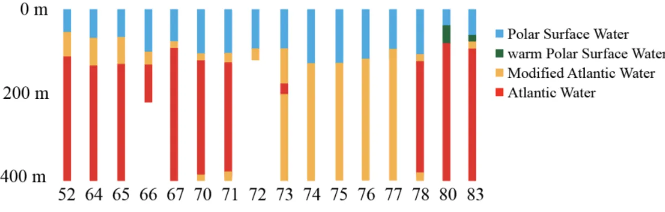
The study area is characterized by an inflow of AW from the Nordic seas and also by typical shelf water masses. Polar Surface Water (PSW) constituted the surface layer between the surface and about 50 to 150 m depth. Atlantic Water (AW) from below reached until a minimum depth of about 80 m. In-between these two water masses were the mixed products warm Polar Surface Water (wPSW) and Modified Atlantic Water (MAW) (Nikolopoulous et al. 2018). During the expedition PS 106/2 the AW reached up close to 100 m depth at the stations 52, 64, 65, 67, 70, 71, 78, 80 and 83 (Figure 2, 3). They were categorized as Atlantic- influenced stations. At the remaining stations 72, 73, 74, 75, 76 and 77, the AW stayed well below 400 m and the PSW layer reached as far down as about 150 m. These stations were categorized as polar-influenced stations.
Station Date Time [UTC] Latitude Longitude Bottom depth (m)
52 29-06-2017 14:41 80.82638 31.953966 135
64 01-07-2017 14:48 81.41416 32.612201 204.4
65 02-07-2017 04:43 81.59516 33.207016 553
67 03-07-2017 12:18 81.95435 32.330701 2818.3
70 05-07-2017 20:58 83.11927 32.924238 3813.4
71 06-07-2017 05:32 83.334 33.237782 3902.6
72 06-07-2017 12:39 83.50125 32.981169 3982.7
73 07-07-2017 10:38 83.71395 32.337495 4022.3
74 08-07-2017 12:26 83.4679 28.085239 4049.1
75 09-07-2017 10:08 82.96345 25.135079 4045.9
76 10-07-2017 08:25 82.48965 18.224139 2277.8
77 10-07-2017 17:15 82.2445 17.782107 2024.9
78 11-07-2017 03:32 82.05043 17.643661 3155.8
80 12-07-2017 19:25 81.43483 17.034591 1849.4
83 13-07-2017 12:15 81.24548 18.605507 472.1
Figure 3: Water masses of upper 400 m at all station, hydrographic information by A. Nikolopoulos (unpublished data)
2.2 Sample analysis
After the samples were rinsed thoroughly with tap water to remove the formaldehyde, each sample was poured through a tower of sieves with decreasing mesh sizes (4000 μm, 2000 μm, 1000 μm, 500 μm, 250 μm, 125 μm, 64 μm) for size fractioning. The sieve tower was the same one that was used to separate the dry mass samples on board. This procedure allows an examination of the taxonomic composition separately within different size classes for later comparison with size-fractionated dry mass data.
The organisms of each subsample were transferred into a beaker prior to the scanning process.
Subsamples with a high abundance of organisms were further split up into aliquots by a plankton splitter (Motoda 1959). The maximal split ratio was 1/256, no replicas were made.
To prevent superimposing animals on each other, it is recommended not to scan more than 1000-1500 organisms with the largest frame. However, this depends heavily on the body size of the organisms (Gorsky et al. 2010). To consider rare species it is recommended to use a sample size that is large enough to include at least a few individuals of every taxon (Grosjean et al. 2004). Therefore, the usage of varying mesh sizes which facilitates subsequent splitting, allowed for reducing the total amount of splits and the examination of larger sample sizes than otherwise possible (Vandromme et al. 2012).
2.3 ZooScan image analysis
We used a ZooScan (Model Biotom, Hydroptic, France) with a resolution of 2400 dpi (Gorsky et al. 2010). A transparent frame of the size of 15x24 cm was attached inside the waterproof flatbed scanner ZooScan. This frame determines the imaging area and allows processing the scan as a single image. The subsamples were then subsequently poured into the scanning cell. The frame has a 5 mm step and water is added above for avoiding the formation of a meniscus (Gorsky et al. 2010). Hereinafter all overlapping organisms were manually separated before the sample was scanned.
Lamps are integrated inside the top cover of the scanner to illuminate the chamber evenly.
The cover also houses a reference cell for optical density. The transparent base of the scanner contains a high-resolution imaging device that permits scanning at a resolution of 2400 dpi.
The base can be hinged which allows the recovery of the subsample without damage through a drainage channel after scanning (Gorsky et al. 2010). After scanning, all the samples were stored in 70% ethanol for further analysis or extended storage after the scanning process.
The images were then analyzed with the software application ZooProcess, a dedicated
imaging software written in Java language for ImageJ and allowing automated processing and measurement of the scanned images. ZooProcess links the images with associated metadata and cuts the scanned image into multiple single images that ideally show no more than one organism (Gorsky et al. 2010). Images that still contain multiple or overlapping organisms were cut manually in the software and processed again.
The single images were uploaded into the web-based database EcoTaxa (Picheral et al. 2017), where they are automatically sorted by a two-way algorithm (random forest algorithm) and manually validated afterwards. An already existing Arctic learning set was used for the first automatic validation. This learning set included a collection of samples from the Fram Strait, containing almost all the taxa that would be expected in the samples of this study. The
precision rate of automatic validation achieved an average of 60% (detailed information on all categories, recall and precision rate can be found in Figure A.1 A.2 and Table A.4), therefore a manual validation afterwards was necessary. Combined with the manual validation
afterward, this semi-automatic process allows a more rapid classification of zooplankton compared to microscopy (Benfield 2007).
The organisms were classified to the lowest taxonomic level possible. Most copepods were determined up to genus level. In some cases, it was also possible to determine up to species level and different life stages (Table A.1/A.2). The 28046 classified images included 13558 non-biotic categories such as detritus, feces, artefact, fiber, and air bubbles. These categories were not considered in the analysis. Likewise, fallen antennas and legs, which made up 3470 images, were not included.
2.4 Abundance, Biovolume and Biomass
For further analysis, the image metadata acquired through EcoTaxa was exported into a tab- separated ASCII table.
To calculate the abundance, the option to export a summary with a count per category (taxon) and sample (i.e. size fraction) was chosen. It should be noted that each row of the table is a group (representing a taxon) of objects scanned by the ZooScan. A row contains the number of organisms scanned within the sample and annotated to this group. Each column of the table is one variable. The number of organisms per group and sample was then added up to
represent the number of organisms for every group within one station.
Next, the abundance was calculated for every taxon of every station by multiplying the
number of organisms with the on-board split ratio (as denominator, i.e. 2) and subsample ratio (as denominator, i.e. 64) from the lab. Next, it was divided by the water volume filtered during the haul.
𝐴𝑏𝑢𝑛𝑑𝑎𝑛𝑐𝑒 = 𝐴𝑏𝑑 *+,-./0 =,1.234 67 6489,+:.: ∗ :<=+>?49>+6 ∗ :12:9.<=3 49>+6
@6=1.3 [./] (1)
A general export through EcoTaxa with the enabled options Object Data, Process Data, Acquisition Data and Sample Data was made for a calculation of biovolume. Each line of the table constitutes one object scanned by the ZooScan and each column of the table constitutes one variable.
An ellipsoid is considered the best representation of many organisms, including abundant copepods. Therefore, the elliptical model was chosen for the calculation of the biovolume, as it appears more realistic. Because the model is a function of both the projected size and the shape of each object and not only a function of the projected size (Vandromme et al. 2012).
The primary axis for the best fitting ellipse of the object (major) and the secondary axis of the best fitting ellipse of the object (minor) were provided by EcoTaxa.
𝑆𝑝ℎ𝑒𝑟𝑖𝑐𝑎𝑙 𝑉𝑜𝑙𝑢𝑚𝑒 = 𝑉 (𝑚𝑚M) = OM∗ ∏ ∗ [ Q9R64 (..)S ∗Q+,64 (..)S ∗Q+,64 (..)S ] (2)
In the next step the spherical volume was multiplied with the subsample ratio (as
denominator, i.e. 64) and split ratio (as denominator, i.e. 2) and then divided with the filtered water volume.
𝐵𝑖𝑜𝑣𝑜𝑙𝑢𝑚𝑒 = 𝐵𝑣 V...//W =X∗:<=+>?49>+6∗:12:9.<=3 49>+6
@6=1.3 [./] (3)
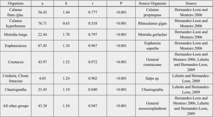
Dry weight was calculated using the regressions between body area of an individual and its dry weight (Lehette and Hernandez-Leon 2009).
𝐷𝑟𝑦 𝑤𝑒𝑖𝑔ℎ𝑡 (𝐷𝑊) =9∗_abbb`(4)
The area (mm2) of each individual was acquired by the image metadata through EcoTaxa and represented by A (the values of “area excluded” were used, in which the white areas within the object are excluded). a and b are the coefficients used following Table 2.
Table 2: Regression and correlation parameters obtained from Lehette and Hernandez-Leon (2009)
Due to high variability in the taxonomy, many groups did not fit the regression line of the coefficients of general mesozooplankton, therefore various coefficients for different groups were used. The coefficients of salps sp. were used as most representative for gelatinous organisms like Cnidaria and Clione limacina based on the findings of Giering et al. (2019).
Biomass density was then calculated by multiplying the DW with the split-ratio (as
denominator, i.e. 2) and subsample ratio (as denominator, i.e. 64) and then dividing with the filtered water volume
𝐵𝑖𝑜𝑚𝑎𝑠𝑠 𝑑𝑒𝑛𝑠𝑖𝑡𝑦 = 𝐵𝑚 V.8./W = de∗:<=+>?49>+6∗:12:9.<=3 49>+6
@6=1.3 [./] (5)
The biomass of each taxon at one station was estimated as the sum of the individual biomasses from every organism.
Organism a b r P Source Organism Source
Calanus
finm./glac. 56.43 1.44 0.777 <0.001 Calanus
propinquus
Hernandez-Leon and Montero 2006 Calanus
hyperboreus 76.71 0.63 0.518 <0.001 Rhincalanus gigas Hernandez-Leon and Montero 2006 Metridia longa 22.44 1.78 0.797 <0.001 Metridia gerlachei Hernandez-Leon and
Montero 2006
Euphausiacea 87.45 1.34 0.967 <0.001 Euphausia
superba
Hernandez-Leon and Montero 2006
Crustacea 43.97 1.52 0.972 <0.001 General
crustaceans
Hernandez-Leon and Montero 2006, Lehette
and Hernandez-Leon, 2009 Cnidaria, Clione
limacina 4.03 1.24 0.902 <0.001 Salps sp. Lehette and Hernandez-
Leon, 2009
Chaetognatha 23.45 1.19 0.840 <0.001 Chaetognatha Lehette and Hernandez-
Leon, 2009
All other groups 43.38 1.54 0.947 <0.001 General
mesozooplankton
Hernandez-Leon and Montero 2006, Lehette
and Hernandez-Leon, 2009
2.5 Statistical analysis
The Mann-Whitney-U test, also called Wilcoxon rank sum test (Wilcoxon 1945) was used to test the significance of differences between the median value of two groups for different parameters (Table A.3). This is a non-parametric test that compares two unpaired groups, more precisely the distribution of ranks in two groups. H0 states that the two groups are part of one population, the rank distributions of values in both groups are identical. The p-value describes the probability that H0 is confirmed. The level of significance α constitutes the p- value below which the probability that the two groups belong to a single population is considered so low that a “significant difference” is assumed, and the null hypothesis (H0) is rejected. For the purpose of this study, α was set to 0.05, following a widely used convention.
Statistical analysis was carried out using the IBM SPSS Statistics software.
The Shannon-Wiener species diversity index (Shannon and Weaver 1949) is defined as 𝐻g = − ∑(𝑝+ ∗ 𝑙𝑜𝑔(𝑝+)) (6)
with ni being the number of individuals of a species i and pi = ,j
k representing the share of a species compared to the total individual number (N) in a sample.
Pielou’s evenness (Pielou 1969) is defined as 𝐽g = mnmg.9o(7)
Where H’ is the number derived from the Shannon-Wiener diversity and H’max is the maximum possible value of H’, equal to H’max = ln(S). With S being the total number of species.
In order to reveal similarities and dissimilarities in the community structure between stations in the study area, a cluster analysis was performed. The abundances of all taxa found at the stations were analyzed. The cluster analysis was performed with R version 1.2.5019 (R Core Team 2020) using the vegan (Oksanen et al. 2013) and graphics (R Core Team 2020) packages. The abundance data was log transformed and a hierarchical clustering of the zooplankton abundance and species composition was carried out for Bray-Curtis-Similarity
3 Results
3.1 Description of the taxa, community composition and taxa abundance
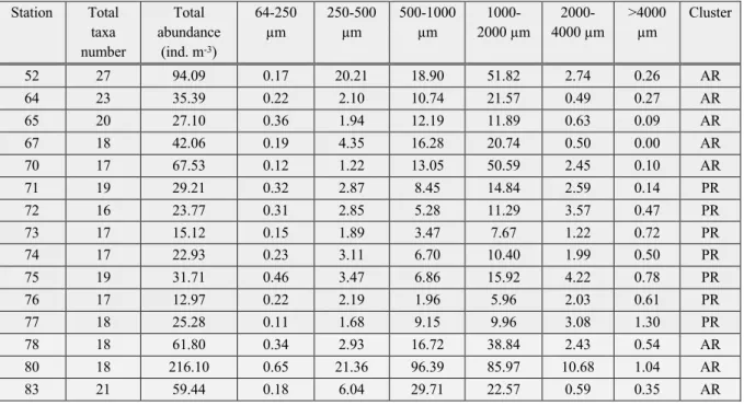
The mesozooplankton community from the shelf of the Barents Sea to the Nansen Basin proper was clearly dominated by copepods. Calanus finmarchicus/glacialis and Calanus hyperboreus were the dominant copepod species. The non-copepod community was mainly composed of Chaetognatha, Appendicularia, Amphipoda, Euphausiacea, Cnidaria, Isopoda and Ostracoda.The highest abundance was recorded at station 80 (216 ind. m-3) in the Sophia Basin. This was followed by station 52 on the shelf (94 ind. m-3). The lowest abundance was found at station 76 (13 ind. m-3) in the Nansen Basin. Overall, the stations with the lowest abundance were all found in the Nansen Basin (Table 3, Figure 1).
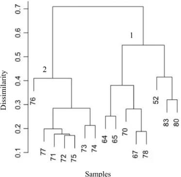
The cluster analysis, based on Bray-Curtis dissimilarity, revealed two different clusters (Figure 4). Cluster 1 contains all stations strongly influenced by AW within 20 m of the depth range sampled in this study. Cluster 2 is separated from the other cluster at a dissimilarity of 0.7 and consists of stations where the AW was well below the sampling depth of the RMT, because layers of Polar Surface Water and Modified Atlantic water overlaid the AW (Figure 2). Only Station 71 was grouped together with these stations although at this station the AW did almost reach the sampling depth of the RMT (Figure 2). Henceforth, Cluster 2 will be referred to as the polar regime (PR) and Cluster 1 as Atlantic regime (AR).
Figure 4: Results of cluster analysis of 15 stations (samples), analysis based on Bray Curtis similarity. With cluster numbers 1 and 2.
Samples
Dissimilarity
The AR contains all stations situated on the shelf or influenced by the shelf slope. Only Stations 70 and 78 were situated in the deeper Nansen Basin. Stations of the AR had
significantly higher overall abundances than the stations of the PR (Mann-Whitney U test; W
= 30, p = 0.001, Table A.3).
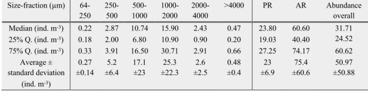
Concerning the abundance of mesozooplankton in the study area, both a spatial and a size- dependent pattern were observed.
At most stations, the relative abundance was dominated by the 1000-2000 µm size-fraction (average 49.7%). Only at station 65, 80 and 83 on the shelf slope, relative abundances in the 500-1000 µm size-fraction (45%, 50%, 45% respectively) were slightly higher than the 1000- 2000 µm size-fraction (44%, 38%, 40% respectively).
At stations 52 and 70 the total abundance of size-fraction 1000-2000 µm was 3 to 4 times higher than the next highest size-fraction. At station 52 and 80 the total abundance of the 250- 500 µm size-fraction was noticeably above-average (Table 3, Figure 5).
Table 3: Total number of taxa and combined abundance of all taxa at the sampling sites. Split in size-fractions.
Station Total taxa number
Total abundance
(ind. m-3)
64-250 µm
250-500 µm
500-1000 µm
1000- 2000 µm
2000- 4000 µm
>4000 µm
Cluster
52 27 94.09 0.17 20.21 18.90 51.82 2.74 0.26 AR
64 23 35.39 0.22 2.10 10.74 21.57 0.49 0.27 AR
65 20 27.10 0.36 1.94 12.19 11.89 0.63 0.09 AR
67 18 42.06 0.19 4.35 16.28 20.74 0.50 0.00 AR
70 17 67.53 0.12 1.22 13.05 50.59 2.45 0.10 AR
71 19 29.21 0.32 2.87 8.45 14.84 2.59 0.14 PR
72 16 23.77 0.31 2.85 5.28 11.29 3.57 0.47 PR
73 17 15.12 0.15 1.89 3.47 7.67 1.22 0.72 PR
74 17 22.93 0.23 3.11 6.70 10.40 1.99 0.50 PR
75 19 31.71 0.46 3.47 6.86 15.92 4.22 0.78 PR
76 17 12.97 0.22 2.19 1.96 5.96 2.03 0.61 PR
77 18 25.28 0.11 1.68 9.15 9.96 3.08 1.30 PR
78 18 61.80 0.34 2.93 16.72 38.84 2.43 0.54 AR
80 18 216.10 0.65 21.36 96.39 85.97 10.68 1.04 AR
83 21 59.44 0.18 6.04 29.71 22.57 0.59 0.35 AR
Table 4: Abundance of all Copepods at the sampling sites. Split in size-fractions.
.
Table 5: Abundance of all taxa within different size-fractions, both Clusters and overall in ind. m-3, median, 25%, 75%
quantile (Q.) and average with standard deviation.
In total the mesozooplankton community of the study area consisted of 34 taxa, 17 of which were classified as copepod species and 17 were non-copepod taxa. 26.5% of all taxa appeared at all stations. More than half of all taxa (56%) appeared at 8 or more stations. The highest number of taxa appeared at Station 52 (27 taxa), followed by the other stations situated on the shelf or influenced by the shelf slope (20-23 taxa). Stations 71 and 75 had the highest number in the Nansen Basin with 19 taxa. The lowest number of taxa was at station 72 with 16 taxa.
(Table A.1/A.2). The number of taxa of stations in the AR (average 19.4) was significantly higher than the number of taxa of stations in the PR (average 16.4) (Mann-Whitney U test; W
= 37, p = 0.029, Table A.3).
Station Total abundance
Copepods (ind. m-3)
64-250 µm
250-500 µm
500-1000 µm
1000- 2000 µm
2000- 4000 µm
>4000 µm
Cluster
52 90.77 0.15 19.81 18.15 50.00 2.57 0.09 AR
64 33.85 0.18 1.75 10.31 21.22 0.35 0.04 AR
65 23.83 0.30 1.37 10.04 11.53 0.54 0.05 AR
67 38.69 0.16 3.79 14.40 19.90 0.44 0.00 AR
70 58.92 0.09 0.67 8.85 47.19 2.10 0.02 AR
71 24.27 0.29 2.19 6.11 13.82 1.84 0.02 PR
72 19.33 0.26 1.81 3.52 10.36 3.26 0.12 PR
73 11.76 0.12 1.34 2.07 6.76 1.14 0.33 PR
74 17.25 0.18 2.25 2.76 9.93 1.89 0.24 PR
75 26.67 0.30 2.80 3.63 15.61 3.94 0.39 PR
76 9.18 0.17 1.24 0.56 4.97 1.90 0.34 PR
77 18.22 0.07 0.68 5.23 9.21 2.52 0.51 PR
78 54.33 0.24 2.00 15.03 34.83 2.04 0.19 AR
80 202.47 0.49 19.28 92.74 80.24 9.51 0.21 AR
83 55.8 0.17 4.99 28.55 21.63 0.33 0.13 AR
Size-fraction (µm) 64- 250
250- 500
500- 1000
1000- 2000
2000- 4000
>4000 PR AR Abundance overall Median (ind. m-3)
25% Q. (ind. m-3)
0.22 0.18
2.87 2.00
10.74 6.80
15.90 10.90
2.43 0.90
0.47 0.20
23.80 19.03
60.60 40.40
31.71 24.52 75% Q. (ind. m-3) 0.33 3.91 16.50 30.71 2.91 0.66 27.25 74.17 60.62
Average ± standard deviation
(ind. m-3)
0.27
±0.14 5.2
±6.4 17.1
±23
25.3
±22.3 2.6
±2.5
0.48
±0.4
23
±6.9
75.4
±60.6
50.97
±50.88
Figure 5: Taxonomic composition at all stations. Abundances (left panel) and relative abundances (right panel). Copepoda with a contribution < 4% are grouped as “Other Copepoda” and non-copepod taxa with contribution <1% are grouped as
“Other Taxa.
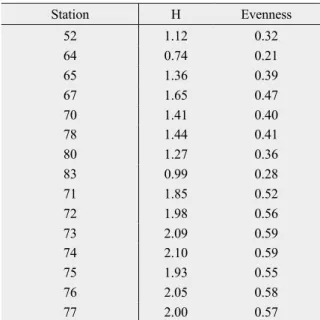
The diversity index of Shannon Wiener (H) and evenness were calculated for all stations (Table 6). The highest H was found at station 74 (2.10) and station 73 (2.09), respectively as well as the highest evenness with 0.59 at both stations. The lowest H was found at station 64 (0.74), as well as the lowest evenness with 0.21. The H and evenness values of the PR stations were significantly higher than values of the AR stations. (Mann-Whitney U test; W = 36, p <
0.001, Table A.3).
Table 6: Shannon-Wiener Index and Evenness of all stations 0
50 100 150 200 250
52 64 65 67 70 78 80 83 71 72 73 74 75 76 77 Abundance (ind m-3)
0%
10%
20%
30%
40%
50%
60%
70%
80%
90%
100%
52 64 65 67 70 78 80 83 71 72 73 74 75 76 77
Relative Abundance (%)
Station H Evenness
52 1.12 0.32
64 0.74 0.21
65 1.36 0.39
67 1.65 0.47
70 1.41 0.40
78 1.44 0.41
80 1.27 0.36
83 0.99 0.28
71 1.85 0.52
72 1.98 0.56
73 2.09 0.59
AR PR AR PR
3.2 Copepods
Copepods dominated the mesozooplankton community at all stations and accounted for 89.65% of the overall abundance in the study area. The distribution varied slightly across the investigation area.
The copepod community consisted of 17 identified taxa, from 12 different families, as well as unidentified Copepoda, Calanoida and nauplii that could not be determined to species level.
However, these unidentified taxa only contributed 2.5% of the total copepod community.
Male copepods accounted for less than 0.05% to the mesozooplankton community and were therefore combined with the females of their respective taxon.
Table 7: Abundance of copepods at all stations, median, quartile (Q.) and average (Avr.) with standard deviation (SD) of all taxa in ind. m-3,
Station Calanus finm./glac.
Calanus hyperboreus
Metridia longa
Other Calanoida
Other Copepoda
Nauplii
52 64.07 3.25 1.91 18.97 1.48 0.22
64 27.62 0.66 2.61 1.73 0.78 0.16
65 18.59 1.25 0.06 1.70 0.94 0.07
67 23.12 2.37 5.58 3.96 2.61 0.00
70 39.78 8.29 8.26 2.07 0.12 0.00
78 37.17 2.56 10.26 2.09 1.51 0.08
80 139.88 3.13 37.06 15.89 4.23 1.24
83 47.15 1.11 1.88 2.85 2.13 0.70
71 13.52 3.44 3.17 1.68 1.84 0.00
72 8.05 6.00 2.02 1.23 1.29 0.21
73 4.57 2.18 2.66 0.94 0.83 0.06
74 5.45 4.35 3.74 1.01 2.15 0.17
75 9.15 5.54 8.24 0.61 2.40 0.20
76 1.22 2.34 3.75 0.19 1.24 0.18
77 10.31 3.31 2.24 1.18 0.40 0.22
Median 18.59 3.13 3.17 1.70 1.48 0.17
25% Q. 8.60 2.26 2.13 1.10 0.88 0.07
75% Q. 38.47 3.89 6.91 2.47 2.14 0.21
Avr.±SD 29.98±35.37 3.32±2.03 6.23±8.99 3.74±5.66 1.60±1.03 0.23±0.33
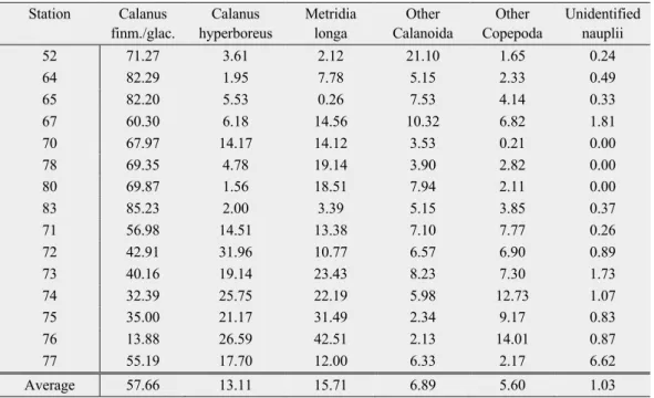
Table 8: Total relative abundance of copepods at each station in %
The highest abundance of copepods was found at station 80 (202.47 ind. m-3), followed by station 52 (90.76 ind. m-3). The lowest abundance of copepods appeared at station 73 (11.77 ind. m-3) and 76 (9.18 ind. m-3) (Table 7). Overall, the stations with the lowest abundance of copepods were all found at stations in the PR (Mann-Whitney U test; W = 30, p = 0.001, Table A.3).
Calanus finmarchicus/glacialis, Calanus hyperboreus and Metridia longa dominated at all stations, compared to other Calanoida and other Copepoda. The AR was characterized by a dominance of Calanus finmarchicus/glacialis, while the PR was characterized by Metridia longa and Calanus hyperboreus. The relative abundance of C. finm./glac. in the PR was lower than in the AR (Mann-Whitney U test; W = 26, p < 0.001, Table A.3), and vice versa for C.
hyperboreus (Mann-Whitney U test; W = 36, p < 0.001, Table A.3).
Station Calanus finm./glac.
Calanus hyperboreus
Metridia longa
Other Calanoida
Other Copepoda
Unidentified nauplii
52 71.27 3.61 2.12 21.10 1.65 0.24
64 82.29 1.95 7.78 5.15 2.33 0.49
65 82.20 5.53 0.26 7.53 4.14 0.33
67 60.30 6.18 14.56 10.32 6.82 1.81
70 67.97 14.17 14.12 3.53 0.21 0.00
78 69.35 4.78 19.14 3.90 2.82 0.00
80 69.87 1.56 18.51 7.94 2.11 0.00
83 85.23 2.00 3.39 5.15 3.85 0.37
71 56.98 14.51 13.38 7.10 7.77 0.26
72 42.91 31.96 10.77 6.57 6.90 0.89
73 40.16 19.14 23.43 8.23 7.30 1.73
74 32.39 25.75 22.19 5.98 12.73 1.07
75 35.00 21.17 31.49 2.34 9.17 0.83
76 13.88 26.59 42.51 2.13 14.01 0.87
77 55.19 17.70 12.00 6.33 2.17 6.62
Average 57.66 13.11 15.71 6.89 5.60 1.03
Figure 6: Species composition of copepods at all stations. Abundances (left panel) and relative abundances (right panel).
Copepods with contribution <4% were grouped as “Other Copepoda”, Calanoida with contribution <3% were grouped as
“Other Calanoida”.
3.3 Selected copepod taxa
Hereafter, the abundance and stage composition of the dominant taxa C.
finmarchicus/glacialis, C. hyperboreus and Metridia longa are examined in more detail in order to analyze spatial patterns within their stage composition.
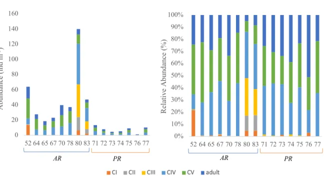
3.3.1 Calanus finmarchicus/glacialis
Calanus finmarchicus/glacialis played a major role in the total copepod community with regard to abundance (Table 8). Similar as for all copepods highest abundances were found at station 80 (139.88 ind. m-3) and 52 (64.07 ind. m-3) and lowest at station 76 (1.22 ind. m-3).
Overall the adult stages, together with the older copepodite stages (copepodite stage CIV) and CV) dominated at most stations, especially in the Nansen Basin. Copepodite stage CIII was abundant at station 80 and 83, while almost being absent at all other stations.
0 50 100 150 200 250
52 64 65 67 70 78 80 83 71 72 73 74 75 76 77 Abundance (ind m-3)
0%
10%
20%
30%
40%
50%
60%
70%
80%
90%
100%
52 64 65 67 70 78 80 83 71 72 73 74 75 76 77
Relative Abundance (%)
AR PR AR PR
In general, copepodite stages CI-CIII showed spatial patterns and were mostly found close to or on the shelf and slope. The highest abundance of stage CII was found at station 80 and 83 (17.41 ind. m-3, 5.93 ind. m-3, respectively) while the highest abundance of stage CI was found at station 52 (13.71 ind. m-3), but CI were also abundant at station 80 and 83 (6.64 ind.
m-3, 2.31 ind. m-3, respectively). Generally, C. finmarchicus/glacialis showed a pattern when comparing the two clusters, by having higher contributions in the AR.
Figure 7: Developmental stage composition of Calanus finmarchicus/glacialis at all stations. Abundances (left panel) and relative abundances (right panel).
3.3.2 Calanus hyperboreus
The adult stages had low contributions ranging from 0.02% to 1.35% on the AR stations and high contributions on the PR stations, with the highest contribution at station 76 with 16.31%.
(Table 8). Stage CV had especially high abundances at station 52 and 70 (2.45 ind. m-3, 4.36 ind. m-3, respectively), while stage CIII had the highest abundance at station 80 (1.04 ind. m-
3), followed by station 70 (0.7 ind. m-3), showing generally higher abundance on the AR stations.
When comparing the two clusters, Calanus hyperboreus had a major contribution at stations
0 20 40 60 80 100 120 140 160
52 64 65 67 70 78 80 83 71 72 73 74 75 76 77 Abundance (ind m-3)
0%
10%
20%
30%
40%
50%
60%
70%
80%
90%
100%
52 64 65 67 70 78 80 83 71 72 73 74 75 76 77
Relative Abundance (%)
AR PR AR PR
Figure 8: Stage composition of Calanus hyperboreus at all stations. Abundances (left panel) and relative abundances (right panel).
3.3.3 Metridia longa
Only the adult stage and CV stage were identified in Metridia longa, with the adult stage being dominant at all stations (except for station 65). Metridia longa showed spatial patterns by having low abundances on the shelf and slope (Table 7). The highest abundance was found at station 80 (37.06 ind. m-3) and the lowest abundance at station 65 (0.06 ind. m-3). The adult stage was absent at station 65, while the CV stage was absent at station 75.
The stage composition of Metridia longa showed no pattern when the two clusters were compared.
0 1 2 3 4 5 6 7 8 9
52 64 65 67 70 78 80 83 71 72 73 74 75 76 77 Abundance (ind m-3)
0%
10%
20%
30%
40%
50%
60%
70%
80%
90%
100%
52 64 65 67 70 78 80 83 71 72 73 74 75 76 77
Relative Abundance (%)
AR PR AR PR