Shelf–Basin interaction along the East Siberian Sea

(1)

www.ocean-sci.net/13/349/2017/

doi:10.5194/os-13-349-2017

Shelf–Basin interaction along the East Siberian Sea

Leif G. Anderson¹, Göran Björk¹, Ola Holby², Sara Jutterström³, Carl Magnus Mörth⁴, Matt O’Regan⁴, Christof Pearce^4,5, Igor Semiletov^6,7,8, Christian Stranne^4,10, Tim Stöven^1,9, Toste Tanhua⁹, Adam Ulfsbo^1,11, and Martin Jakobsson⁴

1Department of Marine Sciences, University of Gothenburg, P.O. Box 461, 40530 Gothenburg, Sweden

2Department of Environmental and Energy Systems, Karlstad University, 651 88 Karlstad, Sweden

3IVL Swedish Environmental Research Institute, Box 530 21, 400 14 Gothenburg, Sweden

4Department of Geological Sciences, Stockholm University, 106 91 Stockholm, Sweden

5Department of Geoscience, Aarhus University, Aarhus, Denmark

6International Arctic Research Center, University Alaska Fairbanks, Fairbanks, AK 99775, USA

7Pacific Oceanological Institute, Russian Academy of Sciences Far Eastern Branch, Vladivostok 690041, Russia

8The National Research Tomsk Polytechnic University, Tomsk, Russia

9Helmholtz Centre for Ocean Research Kiel, GEOMAR, Kiel, Germany

10Center for Coastal and Ocean Mapping/Joint Hydrographic Center, Durham, NH 03824, USA

11Division of Earth and Ocean Sciences, Nicholas School of the Environment, Duke University, Durham, NC 27704, USA Correspondence to:Leif G. Anderson (leif.anderson@marine.gu.se)

Received: 5 December 2016 – Discussion started: 16 December 2016 Revised: 2 April 2017 – Accepted: 3 April 2017 – Published: 27 April 2017

Abstract. Extensive biogeochemical transformation of organic matter takes place in the shallow continental shelf seas of Siberia. This, in combination with brine production from sea-ice formation, results in cold bottom waters with rela- tively high salinity and nutrient concentrations, as well as low oxygen and pH levels. Data from the SWERUS-C3 expedition with icebreakerOden, from July to September 2014, show the distribution of such nutrient-rich, cold bottom waters along the continental margin from about 140 to 180^◦E.

The water with maximum nutrient concentration, classically named the upper halocline, is absent over the Lomonosov Ridge at 140^◦E, while it appears in the Makarov Basin at 150^◦E and intensifies further eastwards. At the intercept between the Mendeleev Ridge and the East Siberian continental shelf slope, the nutrient maximum is still intense, but distributed across a larger depth interval. The nutrient-rich water is found here at salinities of up to∼34.5, i.e. in the water classically named lower halocline. East of 170^◦E transient tracers show significantly less ventilated waters below about 150 m water depth. This likely results from a local isolation of waters over the Chukchi Abyssal Plain as the boundary current from the west is steered away from this area by the bathymetry of the Mendeleev Ridge. The water with salini-

ties of∼34.5 has high nutrients and low oxygen concentrations as well as low pH, typically indicating decay of organic matter. A deficit in nitrate relative to phosphate suggests that this process partly occurs under hypoxia. We conclude that the high nutrient water with salinity∼34.5 are formed on the shelf slope in the Mendeleev Ridge region from interior basin water that is trapped for enough time to attain its signature through interaction with the sediment.

1 Introduction

The extensive, flat, and shallow shelf areas of the Laptev and East Siberian seas are particularly influenced by the changing climate in the Arctic. Coastal erosion from wave action becomes widespread when the summer sea-ice cover shrinks and river discharge increases in warmer humid conditions, both affecting organic matter and nutrient supply (Charkin et al., 2011). At the same time, the decrease in summer sea-ice coverage changes the dynamics of the ocean by increasing vertical mixing and brine production in the fall when sea ice again starts to form over areas that in the past used to be sea-

(2)

ice covered. The changes may impact shelf basin exchange (e.g. Dethleff, 2010; Nishino et al., 2013).

Here we assess data collected in 2014 along the continental shelf break of northern Siberia. Acquired oceanographic and bottom sediment data add to our understanding of water mass modification in the central Arctic Ocean basin. The ob- jectives are to describe the spreading of shelf waters, including those richest in nutrients, from the East Siberian Sea and assess their sources, as well as to evaluate potential effects of diminishing sea-ice coverage under a warmer climate.

The Arctic Ocean has an area of about 9.5×10¹²m²of which more than half is comprised of shallow continental shelf seas (Jakobsson, 2002). The deep central part con- sists of several basins; the Nansen and Amundsen basins are together denoted the Eurasian Basin, and the Canada and Makarov basins constitute the Amerasian Basin. The Lomonosov Ridge stretches from the continental slope of the Laptev Sea to the slope off northern Greenland and separates the Eurasian Basin from the Amerasian Basin (Fig. 1). The deep waters of the Arctic Ocean are supplied from the At- lantic Ocean, entering either through the eastern Fram Strait (Fram Strait Branch, FSB) or over the Barents Sea (Barents Sea Branch, BSB). The latter water flows into the Kara Sea before exiting through the St Anna Trough along the continental margin where it covers a depth range down to about 1500 m (e.g. Schauer et al., 2002). Both branches flow to the east and follow the bathymetry in a cyclonic pattern around the basins (Rudels et al., 1994, Fig. 1), the difference being that the FSB takes the inner turn and is largely restricted to the Eurasian Basin. It is mainly the BSB that flows over the Lomonosov Ridge into the Makarov Basin north of the Laptev Sea.

The upper waters are entering from both the Pacific and Atlantic oceans, where the latter either pass over the Barents shelf or through Fram Strait. The upper waters have classically been divided into a surface mixed layer (SML) that varies seasonally, an upper halocline of mainly Pacific origin, and a lower halocline of Atlantic origin (e.g. Jones and Anderson, 1986; Rudels et al., 1996). The flow pattern of these waters differs. The lower halocline primarily follows the underlying Atlantic layer, while the upper halocline, and even more so the surface mixed layer circulation, is much im- pacted by the dominating wind field (e.g. Jones et al., 2008).

The flow of the surface water is dominated by transport from the Laptev Sea towards Fram Strait, the Transpolar Drift, and one cyclonic circulation in the Canada Basin, the Beaufort Gyre. The size of the latter is determined by the atmospheric pressure field, where a negative Arctic Oscillation results in a larger Beaufort Gyre compared to a positive Arctic Oscil- lation (Proshutinsky et al., 2009).

The properties of the surface mixed layer and the upper halocline are modified over the shelves, and for the SML also in the central Arctic Ocean by, e.g. mixing with river runoff, sea-ice melt, and brine from sea-ice formation. Biogeochem- ical processes also modify the chemical signature, e.g. low-

ering the nutrient concentration of the SML through primary production and increasing the nutrient concentration in the upper halocline through remineralization of organic matter (e.g. Jones and Anderson, 1986). The latter process has been reported to occur in the Chukchi Sea (Bates, 2006; Pipko et al., 2002), East Siberian Sea (Nishino et al., 2009; Anderson et al., 2011), and Laptev Sea (Semiletov et al., 2013, 2016).

One of the most pronounced signatures of the upper halocline of the central Arctic Ocean is a silicate maximum, which was first reported in 1968–1969 from observations made from the drifting T-3 ice island in the Canada Basin (Kinney et al., 1970). In 1979 the silicate maximum was observed during the LOREX study over the Lomonosov Ridge and into the fringe of the Amundsen Basin (Moore et al., 1983). In 1994 no silicate maximum was observed in the Makarov Basin along a section from the Chukchi Sea to the North Pole (Swift et al., 1997). It is clear that the distribution of the upper halocline with its prominent silicate signature has varied much in the past and with changing sea-ice coverage it might vary even more in the future. In this contribution we give some indications of the latter.

Furthermore, recently high silicate concentrations were found at salinities∼34.5 along the continental slope of the eastern East Siberian Sea (Nishino et al., 2009; Anderson et al., 2013). Nishino et al. (2009) suggested that this silicate maximum was produced by decomposition of opal-shelled organisms along the continental margin. Based onδ¹⁸O data collected in 2008, Anderson et al. (2013) reported a brine content of at least 4 % and a small temperature minimum signature associated with the high silicate concentration. The present study will expand on the formation process of this water

2 Methods

Water column data in this study were obtained along six oceanographic sections across the shelf break (A–

F; Fig. 1) during the SWERUS-C3 (Swedish–Russian–

US Arctic Ocean Investigation of Climate–Cryosphere–

Carbon Interactions) expedition in 2014 with Swedish ice- breaker Oden. SWERUS-C3 is a multi-disciplinary international program focusing on investigating the functioning of the Climate–Cryosphere–Carbon (C3) system of the East Siberian Arctic Ocean. The expedition consisted of two legs with the icebreakerOden. Leg 1 started 5 July in Tromsø, Norway, and followed the Siberian continental shelf to end in Barrow, Alaska, on 21 August. Leg 2 took the return route from Barrow and ended in Tromsø on 3 October after con- centrating the field program to the continental shelf break, slope, and the adjacent deep Arctic Ocean basin. Data from leg 2 focusing on the shelf break are discussed in this study.

Water samples were collected using a rosette system equipped with 24 bottles of the Niskin type, each having a volume of 7 L. The bottles were closed during the return of

(3)

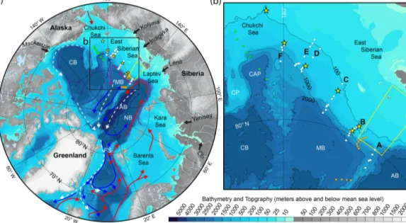
Figure 1.Map of the Arctic Ocean with general currents at intermediate depths over the deep basins and exchange with the surrounding oceans(a). The black frame indicates the investigated area that is illustrated in panel(b)with the hydrographic station positions of sections A to F as white points and those of sediment cores in yellow stars. The Arctic Ocean Section 1994 stations are in green and the orange points show the positions of the ACSYS 96 stations, which are used as historic references. The yellow frame borders the area where the historic sea-ice coverage has been evaluated; see Fig. 10. Abbreviations: Fram Strait (FS), Bering Strait (BS) Nansen Basin (NB), Amundsen Basin (AB), Makarov Basin (MB), Canada Basin (CB), Chukchi Plateau (CP), and Chukchi Abyssal Plain (CAP).

the CTD rosette package from the bottom to the surface and water samples for all constituents were drawn soon after the rosette was secured in the sampling container.

The following constituents are used here: bottle practi- cal salinity, dissolved inorganic carbon (DIC), total alkalin- ity (TA), pH, oxygen, nutrients (NO⁻₃ +NO⁻₂, PO³⁻₄ , SiO₂), and the transient tracer sulfur hexafluoride (SF₆). The order of sampling was determined by the risk of contamination meaning that transient tracer samples were collected first followed by oxygen, the carbon system parameters, nutrients, and salinity.

Salinity and temperature data were collected using a SeaBird 911+CTD with dual SeaBird temperature (SBE 3), conductivity (SBE 04C), and oxygen sensors (SBE 43) at- tached to a 24 bottle rosette for water sampling. Salinity data were calibrated against deep water samples analysed onboard using an Autosal 8400B lab salinometer. The salinometer was calibrated using one standard seawater ampule (IAPSO standard seawater from OSIL Environmental In- struments and Systems) before each batch of 24 samples.

The accuracy of the Autosal salinities and CTD salinities should both be within±0.003 and the accuracy for temperature±0.002^◦C. Water samples for salinity were analysed for more than 90 % of the depth and when no data were available the CTD salinity was used in the evaluation.

The water samples for determination of the transient tracer SF₆ were directly drawn from the Niskin bottles using 250 mL glass syringes. The samples were stored in a cooling bath that was continuously rinsed with cold surface water

to prevent outgassing of the tracers. Measurements were directly performed on board, using a purge and trap GC-ECD system similar to the “PT3” set-up described in Stöven and Tanhua (2014). The column composition was as follows: the trap consisted of a 1/16” column packed with 70 cm Hey- sep D, the 1/8” precolumn was packed with 30 cm Porasil C and 60 cm Molsieve 5Å and the 1/8” main column with 200 cm Carbograph 1AC and 20 cm Molsieve 5Å. The precision for onboard measurements was±0.02 fmol kg⁻¹ for SF₆. In the evaluation of the data, SF₆is given in partial pressure normalized to 1 atm, which is equal to the mixing ratio on the volume scale in parts per trillion (ppt). The advan- tage of using partial pressure instead of concentrations for dissolved gases in the ocean is that the partial pressure is not influence by temperature and salinity effects. The precision is given in concentration since it is related to the absolute value per kg seawater. Age modelling based on these transient tracers is complicated and erroneous at high latitudes due to am- biguous reasons (Stöven et al., 2015, 2016). Hence, we do not provide any statements about the ventilation timescale but rather the ventilation states of the water masses in the Arctic Ocean based on the concentration distribution.

An automated Winkler titration system was used for the oxygen measurements with a precision of ∼1 µmol kg⁻¹. The accuracy was set by titrating known amounts of KIO₃ salts that were dissolved in sulfuric acid. As the amount was known to better than 0.1 % the accuracy should be significantly less than the precision.

(4)

DIC was determined by a coulometric titration method based on Johnson et al. (1987), having a precision of 2.0 µmol kg⁻¹, from duplicate sample analyses, with the accuracy set by calibration against certified reference materi- als (CRM; Batch nos. 123 and 136), supplied by A. Dick- son, Scripps Institution of Oceanography (USA). TA was determined by an automated open-cell potentiometric titration (Haraldsson et al., 1997), with a precision better than 2.0 µmol kg⁻¹ and the accuracy ensured in the same way as for DIC. pH was determined by a spectrophotometric method, based on the absorption ratio of the sulfoneph- talien dye, m-cresol purple (mCP) (Clayton and Byrne, 1993). Purified mCP was purchased from the laboratory of Robert H. Byrne, University of South Florida, USA. The accuracy was estimated to 0.006 from internal consistency calculations of analysed CRM samples and the precision, defined as the absolute mean difference of duplicate samples, was 0.001 pH units. The seawater pH is reported on the total scale and in situ temperature.

The partial pressure of carbon dioxide (pCO₂) was calculated from the combination of pH and TA, and pH and DIC, using CO2SYS version 1.1 (van Heuven et al., 2011) with the stoichiometric dissociation constants of carbonic acid (K^∗₁ and K^∗₂)and bisulfate (K^∗_HSO

4)given by Millero (2010) and Dickson (1990), respectively. Input data included salinity, temperature, PO₄, and SiO₂. The reported values are the average of the two calculated for each sample. The uncer- tainty was computed using a Monte Carlo approach (Legge et al., 2015) and is, expressed as double standard deviation, about 2.5 %.

Besides the extensive sampling and measuring of the water column, analyses were also performed on sediments. Sedi- ment samples from six coring stations along the SWERUS leg 2 cruise track (Fig. 1) were taken from four different depths in the upper 16 cm (Table 1). Two different types of coring devices were used: a gravity corer (GC) and multi- corer (MC). These 24 samples were analysed for biogenic silica (BSi) content, with the aim of investigating a possible sedimentary source of the silicate maximum observed in the water column. Biogenic silica was measured using a wet alkaline extraction technique (Conley and Schelske, 2001). Samples were freeze dried and approximately 30 mg of homogenized sediment was placed in a mild alkaline solu- tion (1 % Na2CO3)at 85^◦C and aliquots were taken at 3, 4, and 5 h during this leaching process. For each of these sub- samples, dissolved Si was measured by Inductively Coupled Plasma Spectrometry, using a Thermo ICAP 6500 DUO. All BSi is assumed to have dissolved after 2 h leaching, after which only Si from minerals is being released. Based on this principle, the zero-hour intercept of the slope from the 3, 4, and 5 h Si concentrations is used to calculate the biogenic fraction. This method was validated by including blanks, and standards from a previous inter-laboratory comparison ex- ercise (Conley, 1998). The relative uncertainties associated with this method are estimated to be±20 % of the measured

value and precision of the ICP is from certified standard measurements better than 5 %.

3 Results

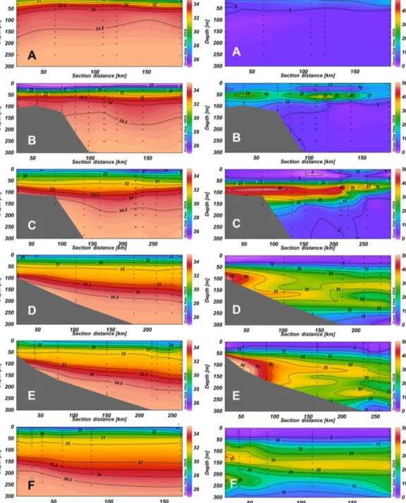
The salinity distribution along the continental margin from the Lomonosov Ridge to the Chukchi Sea shows a similar general pattern, but with some significant variations especially in the top 50 m (Fig. 2). The thinnest layer of low- salinity surface water is found at the Lomonosov Ridge (section A), which increases in thickness eastward in the study area. In section B we find the lowest salinity of 24.55 at 10 m water depth, followed by a very sharp halocline with the salinity increasing from about 32 at 50 m to 34 at 100 m depth. Further to the east the halocline is less sharp with, e.g. the 34 salinity isoline deepening to a depth of more than 200 m. Here, also the > 33 isolines deepens from the shelf towards the deep basin, especially in sections D and E.

The silicate distribution is variable between the sections (Fig. 2). Over the Lomonosov Ridge (section A) the highest silicate concentration, reaching 15 µmol L⁻¹, is found in the surface. In section B the maximum is instead found at about 50 m depth and varies horizontally, with the highest concentration exceeding 30 µmol L⁻¹. At this depth the salinity is around 33. Further to the east at section C, the concentration in the silicate maximum is higher and is found some- what deeper and also at a larger salinity range. It extends horizontally all over the shelf and slope, although with concentrations decreasing some 100–150 km seaward from the shelf break. At the station farthest out in the deep basin the concentration is close to the maximum in section B.

Sections D and E are fairly close to each other and both show a similar pattern. The maximum silicate concentration, above 50 µmol L⁻¹, is close to the bottom at 100–150 m depth (Fig. 2). From here the concentration decreases grad- ually away from the shelf break, to the lowest maximum at the outer station, around 30 µmol L⁻¹. Another specific char- acteristic of the silicate distribution at these sections are the wide depth range of concentrations more than 15 µmol L⁻¹. Here it spans the range of about 50 to 250 m, whereas in section C it only spans 50 to 150 m. To some degree this is attributed to the more gradual increase in salinity with depth, but there are also high concentrations at salinities above 34.5.

In section F the silicate concentration is lower and also spans a narrower depth range. However, this section starts further away from the shelf break and may be difficult to compare with the other sections.

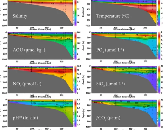
The waters of high silicate concentration have other dis- tinct characters such as high concentrations of the other nutrients, phosphate and nitrate, high apparent oxygen utilization (AOU) andpCO₂, and low pH (Fig. 3). The top 100–150 m is colder than 0^◦C and the nutrient maximum as represented by phosphate is largely confined to the coldest water. There are some small differences in the exact pattern of the differ-

(5)

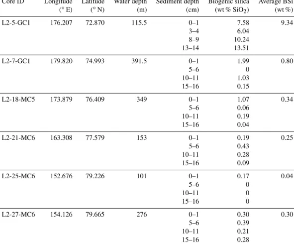
Table 1.Geographic information of sediment cores and their biogenic silica content.

Core ID Longitude Latitude Water depth Sediment depth Biogenic silica Average BSi

(^◦E) (^◦N) (m) (cm) (wt % SiO₂) (wt %)

L2-5-GC1 176.207 72.870 115.5 0–1 7.58 9.34

3–4 6.04

8–9 10.24

13–14 13.51

L2-7-GC1 179.820 74.993 391.5 0–1 1.99 0.80

5–6 0

10–11 1.03

15–16 0.15

L2-18-MC5 173.879 76.409 349 0–1 1.07 0.34

5–6 0.06

10–11 0.19

15–16 0.04

L2-21-MC6 163.308 77.579 153 0–1 0.19 0.25

5–6 0.43

10–11 0.28

15–16 0.09

L2-25-MC6 152.676 79.226 101 0–1 0.17 0.04

5–6 0

10–11 0

15–16 0

L2-27-MC6 154.126 79.665 276 0–1 0.30 0.30

5–6 0.39

10–11 0.21

15–16 0.28

ent parameters, e.g. the AOU maximum is located slightly deeper than that of phosphate farthest out in the deep basin.

Biogenic silica concentrations in the analysed sediments varied widely between the different sites. The full names of the cores include the prefix SWERUS-L2, which hence- forth is omitted. The most western sites (coring stations 21MC1, 25MC1, 27MC1 ∼ water column sections A, B, C) had BSi levels of less than 0.5 % (Fig. 4). Values in- creased slightly to the east, reaching up to 1 % BSi in station 18MC1 (∼water column section D) and up to 2 % in station 7GC1 (∼section F). Concentrations in the most eastern station 5GC1 located on the western flank of Herald Canyon are, however, much higher and reach up to 13.5 %. The surface generally contains the highest concentration of BSi at all sites, except for station 5GC1 where the concentration increases down core. These subtler differences should however be treated with caution due to the large uncertainties associated with the measurement method.

The mean mixed layer partial pressure of SF₆ along all sections is∼8.1 ppt (Fig. 5), which is slightly below the con- temporaneous atmospheric value of 8.4 ppt. At all sections except A, a SF₆minimum is associated with the maximum in AOU. Close to the shelf in section B this SF6 minimum

is 6.4 ppt at 80 m and shoals polewards to 50 m with increasing partial pressure to the range 6.7–7 ppt. The elevated AOU values are 75–138 µmol kg⁻¹at these depths. The SF₆minimum becomes more significant at section C with partial pressures between 4.5–5.1 ppt at 95–130 m (135–183 µmol kg⁻¹ AOU). The maximum deepens eastwards to about 200 m at sections D, E, and F with partial pressures between 2.5–

3.4 ppt and 90–118 µmol kg⁻¹AOU.

The SF6partial pressure in the AW (Atlantic Water) layer between 250 and 600 m is homogeneously distributed with a mean value of about 6 ppt at sections B and C (Fig. 5). In contrast, sections D, E, and F show significant lower mean partial pressures of 4.1–3.4 ppt in the same depth interval with the lowest values at section F. Note that the deep SF₆ partial pressures at sections E and F are close to the values in the overlying minimum at 200 m and the minimum can thus not be defined by SF₆data only. However, the minima can clearly be separated by the AOU values since the warm AW layer shows constant low values of about 50 µmol kg⁻¹along all sections.

The bottom water partial pressure of SF₆ has a general trend of decreasing values at a specific isobaths from the west to the east (Fig. 6). The highest partial pressures of 6.1–

(6)

Figure 2.Sections of salinity (left) and silicate in µmol L⁻¹(right) of the upper 300 m of sections A to F; see Fig. 1 for location of sections.

Sections drawn using Ocean Data View (Schlitzer, 2017).

6.9 ppt can be found at section B between 100 and 500 m.

Section C shows increasing partial pressures with depth from 4.6 ppt at 100 m to 6.5 ppt at 500 m, with decreasing values deeper. A similar gradient of 4.4 to 5.7 ppt can be found at sections D, E, and F at the same depth range. Below∼500 m the partial pressure decreases with increasing depth, reaching the detection limit at 1900–2000 m in the Makarov Basin (Fig. 6).

4 Discussion

In section A, the most western that is located over the Lomonosov Ridge, the highest silicate concentrations are found in the surface. Hence, no sub-surface maximum typical of the upper halocline water is present here. The surface silicate maximum is associated with low salinity, which is a typical signature of runoff from the Lena River. Thus, this surface water has a substantial fraction of freshwater from river, even if there also is a contribution of sea-ice melt. The

(7)

Figure 3.Properties in the upper 1000 m along section D of Fig. 1. Sections drawn using Ocean Data View (Schlitzer, 2017).

Figure 4.Biogenic silicate (BSi) concentrations (percent dry weight) in the upper 16 cm of the sediment(a)at coring sites shown in panel(b).

The symbols of the coring sites are colour coded after measured BSi concentration from the lowest concentrations in blue to the highest in red. The black bars represent the depth layer of the sediment that is analysed.

high silicate surface water is also seen in section B and partly in section C but not further to the east, indicating the limit of the river plume to this part of the deep Arctic Ocean.

The highest silicate concentrations are found at the shelf slope of sections D and E and this is also where the salin-

ity isolines shoal (Fig. 2). The increase in salinity along the shelf slope at bottom depths less than 250 m is accompanied by an increase in temperature as illustrated in the depth panels (Fig. 7a and b) with no indication of mixing with another water mass, as all data from these sections have the same

(8)

Figure 5.pSF₆(ppt per volume) profiles from surface to 550 m depth, coloured by AOU (µmol kg⁻¹)of the stations in sections A to F.

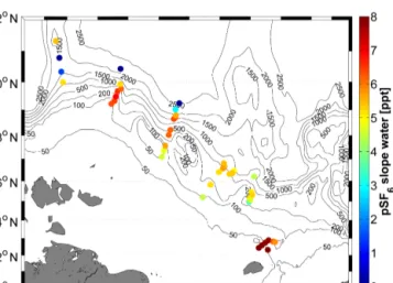
Figure 6.SF₆partial pressure (ppt) in the sample collected closest to the bottom, typically 5–10 m above.

shape in aT−Spanel (Fig. 8a) for salinity > 32.5. The slope of the isolines infers a near-bottom increase of the current due to geostrophic shear, which is superimposed on the typical overall eastward current (e.g. Rudels, 2012). Although it is not possible to determine the absolute current velocity from just a geostrophic calculation, our data together with the known direction of the mean flow suggest that we have a bottom intensified flow in the eastward direction. The mag- nitude of this increase is about 3 cm s⁻¹(based on the den- sity difference and distance between the two slope stations located at 164 and 241 m water depth in section E) over the depth range 100–150 m, which is not negligible.

At sections D and E is the maximum observed silicate concentration about 56 µmol L⁻¹and found at∼120 m (Fig. 7c) but elevated concentrations are found down to nearly 250 m depth. Plotting silicate concentrations against salinity (Fig. 8c) shows a clear pattern with a shallow maximum around 33 and a deep maximum at 34.5. These maxima are also evident in the section panels in Fig. 2.

(9)

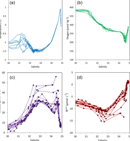
Figure 7.Depth profiles of temperature(a), salinity(b), silicate(c), and N^∗∗(d)in the upper 300 m of all stations at sections D and E; see Fig. 1 for locations.

When the nutrient maximum is accompanied by an oxygen minimum (Fig. 3) it suggests organic matter mineralization, and if this occurs at low oxygen levels, nitrate is lost as electron acceptor via either denitrification or anammox. Such conditions can only be met close to, or in, the sediments of the shelves within the Arctic Ocean as all other waters observed in this region are well oxygenated. A deficit in nitrate is seen when computing the property N^∗∗=0.87×[NO₃]−16×[PO₄]+2.9 (Codispoti et al., 2005), which gives a constant value if the classical Redfield–Ketchum–Richard N : P ratio (Redfield et al., 1963) is followed. A low value indicates denitrification. The N^∗∗

profiles (Fig. 7d) show a broad minimum focused at depths around 100 m, strongly indicating that this water has had its signature influenced by hypoxic conditions, i.e. loss of nitrate when used as electron acceptor during mineralization of organic matter at low oxygen concentration.

More information on the formation history of the high salinity silicate maximum water can be obtained from property versus salinity panels (Fig. 8). TheT−S curve show a typical shape for the halocline, with a warmer low-salinity water at S≈31, followed by a temperature minimum at 32 <S< 33 and then increasing temperature with salinity to a maximum in the Atlantic Layer, followed by colder wa-

ter towards the highest salinity in the deep water (Fig. 8a).

The temperature minimum has historically been attributed to winter water, often with a signature of brine contribution (e.g. Aagaard et al., 1981; Anderson et al., 2013). This brine enhanced water follows the shelf bottom and gets enriched in organic matter decay products during its flow towards the deep basin. A nearly strait mixing line can be seen in the salinity range from aboutS=34 to that of the temperature maximum (Fig. 8a), i.e. noT_minat the high salinity silicate maximum water. Oxygen profiles, on the other hand, show a clear minimum atS≈34.5 (Fig. 8b) indicating organic matter remineralization. Comparing the oxygen signature with those of silicate and N^∗∗(Fig. 8c and d) reveals interesting information. The broad silicate maximum aroundS≈33 has a minimum in N^∗∗but no minimum in oxygen even if the concentration is some 100 µmol kg⁻¹below saturation, while the silicate maximum atS≈34.5 has a clear oxygen minimum but with only a slight minimum in N^∗∗. The most plausible explanation for this pattern is that the nutrient maximum at low salinity had a higher oxygen concentration before ex- posure to organic matter decay at the sediment surface. The waters withS> 34 at some stations with lower oxygen and higher silicate concentrations also have lower N^∗∗(Fig. 8b,

(10)

Figure 8.Temperature(a), oxygen(b), silicate(c)and N^∗∗(d)versus salinity for the stations at sections D and E. The panels(a)and(b)are from the CTD output, while(c)and(d)are from water samples analysed.

c and d), indicating less mixing and thus potentially more recent contact with the sediment surface.

The conclusion is that both nutrient maxima are formed in contact with hypoxic sediments, with one maxima at salinity around S≈33 mainly being formed on the shelf where the preformed water is well oxygenated by interaction with the atmosphere during ice-free periods and ice formation periods with cooling and convection, while the nutrient maximum at S≈34.5 is formed at the shelf break of more than 100 m depth. Such a scenario is consistent with the SF₆partial pressure of the silicate maximum atS≈34.5 being close to those in the deep basin, while that around S≈33 has a significantly higher level of around 7 ppt (Fig. 5). At section B the maximum AOU is associated withS≈33 and found at about 50 m depth (Fig. 5b) and at C it is found at around 100 m depth (Fig. 5c). At the latter section the maximum AOU is found at S≈34.5 associated with the SF₆ partial pressure minimum of around 5 ppt. At the same salinity there is also a weaker minimum in section B at about 75 m depth. In sec-

tions D, E, and F the SF₆minimum is also found atS≈34.5 but at a deeper depth of 200 m, all associated with the AOU maximum. However, at these sections the AOU maximum has a SF₆ partial pressure close to that of the water deeper, indicating that the basin water in the Chukchi Abyssal Plain is the source of this high salinity nutrient maximum water.

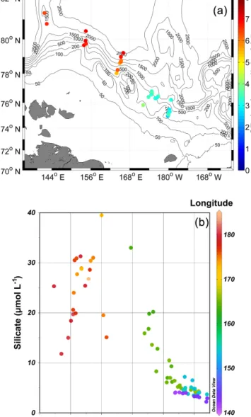
The presence of the high salinity SF6minimum at section C, and to a lesser degree at section B, points to the existence of a westward penetration of water at the shelf break. How- ever, this does not need to be a persistent flow, but can be something that occurs intermittently. Strengthening of these concussions are seen in Fig. 9 where the pSF₆interpolated to a salinity of 34.5 has a strong gradient with increasing partial pressure towards the west and significant higher silicate concentrations at lower pSF₆.

The formation of the silicate maximum atS≈34.5 on the shelf break is in line with Nishino et al. (2009), who suggested that the silicate maximum at this high salinity was produced by decomposition of opal-shelled organisms along

(11)

the continental margin. Anderson et al. (2013) showed that this high salinity silicate maximum had a brine content of at least 4 % and that the CTD record had a small temperature minimum signature. This was not the situation in 2014, illustrating that the conditions likely are not constant with time. This water with a salinity of just over 34 has historically been named lower halocline water (Jones and Ander- son, 1986), without a signature of any nutrient maximum.

Hence, this more recent finding of high silicate concentrations along the continental margin of the East Siberian Sea is either a local or a new phenomenon. The sediment record (Fig. 4) clearly shows that the BSi content is low in the slope off the western part of East Siberian Sea (sections B and C;

coring stations 27MC1, 25MC1, 21MC1), making local decomposition in this region unlikely. Further to the east the BSi content increases slightly to the location of sections D and F, with a large increase at the most eastern station in the Herald Canyon (13.5 % BSi at site 5GC1) where opal- shelled organism, primarily diatoms, are abundant in the bottom sediments. This strongly supports a Pacific Ocean source of silicate, but does not exclude that some of the silicate-rich water enters the eastern East Siberian Sea before transformation and escape to the slope and deep central basins. Such a scenario is consistent with the decreasing silicate concentrations to the west in the salinity range 34.3 to 34.7 (Fig. 9b).

However, it is not possible to fully elucidate the transport and transformation of silicate from these few sediment profiles, especially since they are also from variable bottom depths (Table 1). Nevertheless, these sediment observations do not contradict occasional westward flow along the shelf break, as suggested by the SF6signature.

Variability is also seen in a comparison with historic data.

Our section F is on the border to the Chukchi Abyssal Plain, where the Arctic Ocean Section hydrographic program collected a section of data in 1994. In Fig. 10 we compare these two data sets and it is clear that the silicate maximum at S≈34.5 was more or less absent in 1994. However, at stations with bottom depths∼180 m the silicate concentration was close to 20 µmol L⁻¹towards the seafloor, and at the station with bottom depth∼250 m, the concentration decreased to 18 µmol L⁻¹ towards the seafloor. These are the stations where the salinity does not reach the maximum salinity in Fig. 10a. Hence, there seems to be a signal from the shelf slope that did not penetrate deep into the Chukchi Abyssal Plain. Also N^∗∗had relative to the deepest data higher values atS≈34 except for at the shallowest stations with elevated silicate concentrations (Fig. 10b). Centred atS≈33 the silicate maximum is higher and the N^∗∗minimum is lower in 1994, indicating a stronger contribution of organic matter decay at low oxygen levels from the shelf. There is also an indication of a wider salinity interval of the silicate maximum in 2014 compared to 1994, especially towards the high salinity end (Fig. 10a).

Historically the extent of the nutrient maximum has varied but few studies along the Siberian continental margin

Figure 9. SF₆ partial pressure (ppt) interpolated to the salinity 34.5(a)and silicate versus pSF₆in the salinity range 34.3 to 34.7 colour coded by longitude(b).

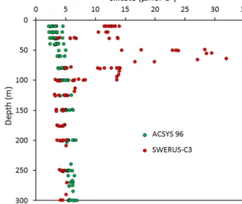
have been reported. Data from east of 175^◦E for years between 2001 and 2010 were compiled by Nishino et al. (2013) showing the presence of the nutrient maximum but with some variability in both the maximum concentration and the vertical extent between the years. Our 2014 data show a clear maximum in the Makarov Basin, at section B some 150 nau- tical miles east of the Lomonosov Ridge at about longitude 153^◦E, with higher concentrations in the sections further to the east (Fig. 2). As the concentration of silicate generally increases towards the shelf in sections B and C and also increases from section B to C (Fig. 2) it is likely that the source is the local shelf area. Data obtained from RVPolarsternin the same area as section B (see Fig. 1b for station locations) during the summer of 1996 (ACSYS 96) did not show any elevated silicate concentrations in the halocline (Fig. 11). This

(12)

Figure 10.Silicate(a)and N^∗∗(b)versus salinity in the Chukchi Abyssal Plain area; data from the Arctic Ocean Section in 1994 in green (stations marked by green points in Fig. 1b) and from SWERUS-C3 in red (section F in Fig. 1b).

could be an effect of either that in 1996 the nutrient-rich water was confined closer to the shelf on its transport to the east, or that the production site of this water has extended further to the west since 1996. We find it most plausible that the latter is the cause as the sea-ice climate has changed significantly over the shelf south of these sections during the last 20 to 30 years (Fig. 12) that potentially have moved the production areas further to the west. Up to about the year 2000 most summers had more than 50 % sea-ice coverage, with a few years with less than 10 %. During the last 10 years the typical conditions for the month of September is more than 90 % open water. All through the record the area is more or less ice covered in November, a situation that lasts until April. Con- sequently, there has been more sea-ice formation and, thus, brine production in this region during the last 10 years compared to the 1980s and 1990s. When this sea-ice formation is further away from the coast line the initial salinity is proba- bly also higher and thus also the resulting brine.

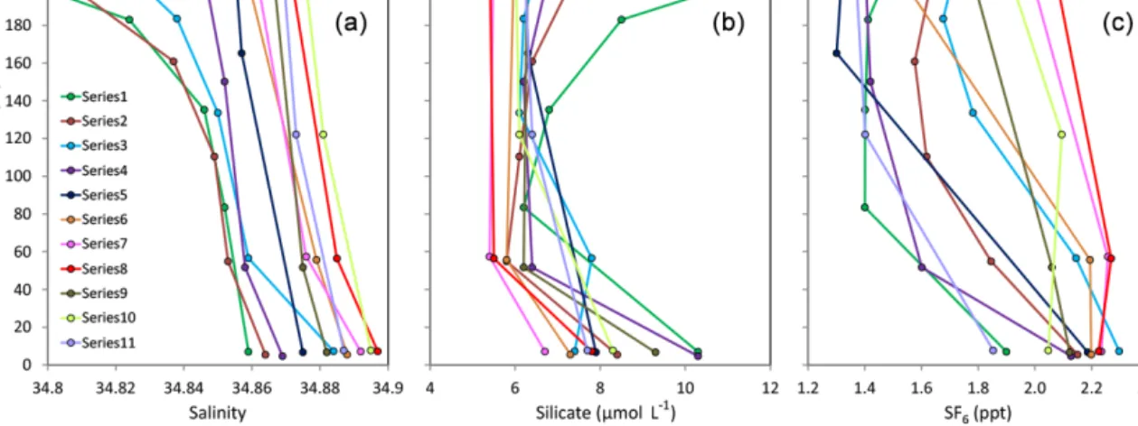
Indications of shelf plumes penetrating all the way to the deep basin are seen in sections D and F where salinity, silicate, and SF₆levels increases towards the bottom, a signa-

Figure 11.Silicate versus depth for data collected in 1996 (green) and from section B in 2014 (red). The positions of the stations in 1996 are shown by orange points in Fig. 1b.

Figure 12.Percentage of ice-free area in the region: latitude 76 to 80^◦N, longitude 140 to 150^◦E (framed yellow in Fig. 1b), for each month from 1980 to 2014, evaluated from the passive microwave data of NSIDC (Cavalieri et al., 1996).

ture that generally fades away down the shelf slope (Fig. 13).

This is not observed in the more western sections and is consistent with shelf plumes penetrating down into this eastern region. A rough computation of the fraction of shelf water can be done as follows. With an increase in SF6 partial pressure from the intermediate to the bottom water of about 0.5 ppt, and the intermediate water and shelf water partial pressures being 1.5 and 8 ppt, respectively, a little less than 10 % of shelf water is needed. This is quite substantial but not unrealistic if matched with the other properties. The shelf water silicate concentration should be∼25 µmol L⁻¹in order to achieve the observed 2 µmol L⁻¹increase, and the shelf water salinity would be 36 to get an increase of 0.15.

These computations completely ignore mixing and entrain-

(13)

Figure 13.Salinity(a), silicate(b), and SF₆(c)as a function of distance from the bottom for all stations deeper than 400 m in sections D and F. Series 1 to 11 represent the bottom depth, increasing from 483 to 1120 m.

ment, but provide some indication that a shelf water contribution to the deep water of the Chukchi Abyssal Plain is realistic. The realism of the shelf source concentrations is supported by observations and modelling. For instance, silicate concentrations in the range 40 to 60 µmol L⁻¹was observed on the western flank of Herald Canyon in the summer of 2008, even if the salinity was well below 34 (Ander- son et al., 2013). Windsor and Björk (2000) used a polynya model driven by atmospheric forcing to compute ice, salt, and dense water production in different regions of the Arctic Ocean over 39 winter seasons from 1959 to 1997. Two regions were east and west of the Wrangle Island where mean salinities of 37.0 and 35.9 were produced, respectively, well within the range needed.

5 Conclusions

We have showed that this region of the Arctic Ocean is much more dynamic and variable than previously reported. Our data collected in the summer of 2014 are consistent with a shelf–basin exchange scenario as summarized in Fig. 14. A boundary current of Atlantic Layer water follows the shelf break from the west to the east, where some of the water crosses the Lomonosov Ridge into the Makarov Basin. This boundary current follows the shelf break to the Alpha Ridge where it turns towards north at its western flank. The water at the corresponding depth in the Chukchi Abyssal Plain has a substantially lower partial pressure of SF₆, consistent with a more isolated circulation in this region.

Surface water with substantial input of river water exits the shelf north of the New Siberian Islands to follow the Lomonosov Ridge out into the central basins. High nutrient water with salinity centred at 33 exits the East Siberian Sea from its western end and contributes to the cold halocline of the central Arctic Ocean. Compared to historic data the high nutrient water is found outside the shelf break further to the

Figure 14.Summary of deduced circulation. Green arrow shows the runoff spreading in the surface out north of the New Siberian Islands. The light brown illustrates the export of nutrient-rich water from the shelf into the deep basin at a salinity of around 33 and the dark brown interrupted line the nutrient-rich water of a salinity around 34.5. The dark blue arrows in the deep basin show the intermediate deep (500–1500 m depth) boundary currents. The yellow dotted line illustrates the deep water plumes off the shelf break.

Map drawn using Ocean Data View (Schlitzer, 2017).

west in 2014, which is associated with a lower degree of ice cover during the summer north of the New Siberian Islands.

Where the Mendeleev Ridge connects to the shelf slope a water body with salinity around 34.5, elevated nutrient concentrations and low SF₆partial pressure hugs the shelf slope.

Water of such property is also found further to the west. As the source of the low SF₆partial pressure most likely is in the Chukchi Abyssal Plain, at least an occasional flow to the west follows, a conclusion that is supported by the surface sediment biogenic silicate (BSi) content. In the eastern study region plumes of high salinity, silicate, and SF₆levels flow off the shelf into the deep basin.

(14)

Data availability. Data are available upon request to the corresponding author.

Competing interests. The authors declare that they have no conflict of interest.

Acknowledgements. We thank the supporting crew and Master of I/BOdenas well as the support of the Swedish Polar Secretariat.

This research was supported by grants from the Swedish Research Council (contract 621-2013-5105); the Swedish Research Council Formas (project reference 214-2008-1383, A.U. 214-2014- 1165); the Swedish Knut and Alice Wallenberg Foundation (KAW);

the European Union FP7 project CarboChange (under grant agree- ment no. 264879). I. Semiletov acknowledge support from the Russian Government (grant no. 14.Z50.31.0012/03/19.2014), the Far Eastern Branch of the Russian Academy of Sciences and the ICE-ARC-EU FP7 project. The transient tracer measurements were supported by the Deutsche Forschungsgemeinschaft in the frame- work of the “Antarctic Research with comparative investigations in Arctic ice areas” priority program by a grant to T. Tanhua and M. Hoppema; Carbon and transient tracers dynamics: a bi-polar view on Southern Ocean eddies and the changing Arctic Ocean (TA 317=5, HO 4680=1).

Edited by: T. Tesi

Reviewed by: S. Nishino and two anonymous referees References

Aagaard, K., Coachman, L. K., and Carmack, E. C.: On the halocline of the Arctic Ocean, Deep-Sea Res., 28, 529–545, 1981.

Anderson, L. G., Björk, G., Jutterström, S., Pipko, I., Shakhova, N., Semiletov, I., and Wåhlström, I.: East Siberian Sea, an Arctic region of very high biogeochemical activity, Biogeosciences, 8, 1745–1754, doi:10.5194/bg-8-1745-2011, 2011.

Anderson, L. G., Andersson, P., Björk, G., Jones, E. P., Jutter- ström, S., and Wåhlström, I.: Source and formation of the upper halocline of the Arctic Ocean, J. Geophys. Res., 118, 410–421, doi:10.1029/2012JC008291, 2013.

Bates, N. R.: Air-sea CO₂fluxes and the continental shelf pump of carbon in the Chukchi Sea adjacent to the Arctic Ocean, J.

Geophys. Res., 111, C10013, doi:10.1029/2005JC003083, 2006.

Cavalieri, D., Parkinson, C., Gloersen, P., and Zwally, H.J.: Sea Ice Concentrations from Nimbus-7 SMMR and DMSP SSM/I- SSMIS Passive Microwave Data, [1996-01-01; 2010-12-31], Na- tional Snow and Ice Data Center, Boulder, Colorado USA, Digi- tal media, updated yearly, 1996.

Charkin, A. N., Dudarev, O. V., Semiletov, I. P., Kruhmalev, A. V., Vonk, J. E., Sánchez-García, L., Karlsson, E., and Gustafsson, Ö.: Seasonal and interannual variability of sedimentation and organic matter distribution in the Buor-Khaya Gulf: the primary re- cipient of input from Lena River and coastal erosion in the south- east Laptev Sea, Biogeosciences, 8, 2581–2594, doi:10.5194/bg- 8-2581-2011, 2011.

Clayton, T. D. and Byrne, R. H.: Spectrophotometric seawater pH measurements: total hydrogen ion concentration scale calibration of m-cresol purple and at-sea results, Deep-Sea Res. Pt. I, 40, 2115–2129, 1993.

Codispoti, L. A., Flagg, C., Kelly V., and Swift, J. H.: Hydrographic conditions during the 2002 SBI process experiments, Deep-Sea Res. Pt. II, 52, 3199–3226, 2005.

Conley, D. J.: An interlaboratory comparison for the measurement of biogenic silica in sediments, Mar. Chem., 63, 39–48, doi:10.1016/S0304-4203(98)00049-8, 1998.

Conley, D. J. and Schelske, C. L.: Biogenic Silica, in: Tracking En- vironmental Change Using Lake Sediments, edited by: Smol, J.

P., Birks, H. J. B., Last, W. M., Bradley, R. S., and Alverson, K., Kluwer Academic Publishers, Dordrecht, the Netherlands, 281–

293, 2001.

Dethleff, D.: Dense water formation in the Laptev Sea flaw lead, J.

Geophys. Res., 115, C12022, doi:10.1029/2009JC006080, 2010.

Dickson, A. G.: Standard potential of the reaction:

AgCl(s)+1/2H₂(g)=Ag(s)+HCl(aq), and the standard acidity constant of the ion HSO⁻₄ in synthetic sea water from 273.15 to 318.15 K, J. Chem. Thermodyn., 22, 113–127, doi:10.1016/0021-9614(90)90074-Z, 1990.

Haraldsson, C., Anderson, L. G., Hassellöv, M., Hulth, S., and Ols- son, K.: Rapid, high-precision potentiometric titration of alkalin- ity in the ocean and sediment pore waters, Deep-Sea Res. Pt. I, 44, 2031–2044, 1997.

Jakobsson, M.: Hypsometry and volume of the Arctic Ocean and its constituent seas, Geochem. Geophys. Geosys., 3, 1–18, 2002.

Johnson, K. M., Sieburth, J. M., Williams, P. J., and Brändström, L.: Coulometric total carbon dioxide analysis for marine studies:

automation and calibration, Mar. Chem., 21, 117–133, 1987.

Jones, E. P. and Anderson, L. G.: On the Origin of the Chemical Properties of the Arctic Ocean Halocline, J. Geophys. Res., 91, 10759–10767, 1986.

Jones, E. P., Anderson, L. G., Jutterström, S., Mintrop, L., and Swift, J. H.: Pacific freshwater, river water and sea ice meltwater across Arctic Ocean basins: Results from the 2005 Beringia Expedition, J. Geophys. Res., 113, C08012, doi:10.1029/2007JC004124, 2008.

Kinney, P., Arhelger, M. E., and Burrell, D. C.: Chemical charac- teristics of water masses in the Amerasian Basin of the Arctic Ocean, J. Geophys. Res., 75, 4097–4104, 1970.

Legge, O. J., Bakker, D. C. E., Johnson, M. T., Meredith, M.

P., Venables, H. J., Brown, P. J., and Lee, G. A.: The seasonal cycle of ocean-atmosphere CO₂ flux in Ryder Bay, west Antarctic Peninsula, Geophys. Res. Lett., 42, 2934–2942, doi:10.1002/2015GL063796, 2015.

Millero, F.: Carbonate constants for estuarine waters, Mar. Fresh- water Res., 61, 139–142, doi:10.1071/MF09254, 2010.

Moore, R. M., Lowings, M. G. and Tan, F. C.: Geochemical profiles in the central Arctic Ocean: Their relation to freezing and shallow circulation, J. Geophys. Res., 88, 2667–2674, 1983.

Nishino, S., Shimada, K., Itoh, M., and Chiba, S.: Vertical Double Silicate Maxima in the Sea-Ice Reduction Region of the West- ern Arctic Ocean: Implications for an Enhanced Biological Pump due to Sea-Ice Reduction, J. Oceanogr., 65, 871–883, 2009.

Nishino, S., Itoh, M., Williams, W. J., and Semiletov, I.: Shoaling of the nutricline with an increase in near-freezing temperature water in the Makarov Basin, J. Geophys. Res.-Oceans, 118, 635–649, doi:10.1029/2012JC008234, 2013.

Pipko, I. I., Semiletov, I. P., Tishchenko, P. Ya., Pugach, S. P., and Christensen, J. P.: Carbonate chemistry dynamics in Bering Strait and the Chukchi Sea, Prog. Ocean., 55, 77–94, 2002.

(15)

Proshutinsky, A., Krishfield, R., Timmermans, M.-L., Toole, J., Car- mack, E., McLaughlin, F., Williams, W. J., Zimmermann, S., Itoh, M., and Shimada, K.: Beaufort Gyre freshwater reservoir:

State and variability from observations, J. Geophys. Res., 114, C00A10, doi:10.1029/2008JC005104, 2009.

Redfield, A. C., Ketchum, B. H., and Richards, F. A.: The influence of organisms on the composition of sea water, in: The Sea, Vol. 2., edited by: Hill, M. N., Wiley, New York, USA, 26–77, 1963.

Rudels, B.: Arctic Ocean circulation and variability – advection and external forcing encounter constraints and local processes, Ocean Sci., 8, 261–286, doi:10.5194/os-8-261-2012, 2012.

Rudels, B., Jones, E. P., Anderson L. G., and Kattner, G.: On the intermediate depth waters of the Arctic Ocean, in: The Po- lar Oceans and Their Role in Shaping the Global Environment, edited by: Johannessen, O. M., Muench, R. D., and Overland, J.

E., American Geophysical Union, Washington, D.C., USA, 33–

46, 1994.

Rudels, B., Anderson, L. G., and Jones, E. P.: Formation and evolu- tion of the surface mixed layer and halocline of the Arctic Ocean, J. Geophys. Res., 101, 8807–8821, 1996.

Schauer, U., Rudels, B., Jones, E. P., Anderson, L. G., Muench, R. D., Björk, G., Swift, J. H., Ivanov, V., and Larsson, A.-M.:

Confluence and redistribution of Atlantic water in the Nansen, Amundsen and Makarov basins, Ann. Geophys., 20, 257–273, doi:10.5194/angeo-20-257-2002, 2002.

Schlitzer, R.: Ocean Data View, available at: http://odv.awi.de, last access: February 2017.

Semiletov, I., Pipko, I., Gustafsson, O., Anderson, L. G., Sergienko, V., Pugach, S., Dudarev, O., Charkin, A., Gukov, A., Broder, L., Andersson, A., Spivak, E., and Shakhova, N.: Acidifica- tion of East Siberian Arctic Shelf waters through addition of freshwater and terrestrial carbon, Nat. Geosci., 9, 361–365, doi:10.1038/ngeo2695, 2016.

Semiletov, I. P., Shakhova, N. E., Pipko, I. I., Pugach, S. P., Charkin, A. N., Dudarev, O. V., Kosmach, D. A., and Nishino, S.: Space–

time dynamics of carbon and environmental parameters related to carbon dioxide emissions in the Buor-Khaya Bay and adjacent part of the Laptev Sea, Biogeosciences, 10, 5977–5996, doi:10.5194/bg-10-5977-2013, 2013.

Stöven, T. and Tanhua, T.: Ventilation of the Mediterranean Sea constrained by multiple transient tracer measurements, Ocean Sci., 10, 439–457, doi:10.5194/os-10-439-2014, 2014.

Stöven, T., Tanhua, T., Hoppema, M., and Bullister, J. L.: Perspec- tives of transient tracer applications and limiting cases, Ocean Sci., 11, 699–718, doi:10.5194/os-11-699-2015, 2015.

Stöven, T., Tanhua, T., Hoppema, M., and von Appen, W.-J.: Tran- sient tracer distributions in the Fram Strait in 2012 and inferred anthropogenic carbon content and transport, Ocean Sci., 12, 319–

333, doi:10.5194/os-12-319-2016, 2016.

Swift, J. H., Jones, E. P., Carmack, E. C., Hingston, M., Macdon- ald, R. W., McLaughlin, F. A., and Perkin, R. G.: Waters of the Makarov and Canada Basins, Deep-Sea Res. Pt. II, 44, 1503–

1529, 1997.

van Heuven, S., Pierrot, D., Lewis, E., and Wallace, D. W. R.:

MATLAB Program developed for CO₂system calculations, version 1.1 2011, ORNL/CDIAC-105b. Carbon dioxide information analysis center, Oak Ridge National Laboratory, U.S. Depart- ment of Energy, Oak Ridge, USA, 2011.

Winsor, P. and Björk, G.: Polynya activity in the Arctic Ocean from 1958 to 1997, J. Geophys. Res., 105, 8789–8803, 2000.