Ocean Modelling

(1)

Contents lists available atScienceDirect

Ocean Modelling

journal homepage:www.elsevier.com/locate/ocemod

Simulating the Agulhas system in global ocean models – nesting vs. multi- resolution unstructured meshes

Arne Biastoch

^a,⁎

, Dmitry Sein

^b

, Jonathan V. Durgadoo

^a

, Qiang Wang

^b

, Sergey Danilov

^b

aHelmholtz-Zentrum für Ozeanforschung Kiel, Kiel, Germany

bAlfred-Wegener Institut, Helmholtz-Zentrum für Polar- und Meeresforschung (AWI), Bremerhaven, Germany

A R T I C L E I N F O

Keywords:

Unstructured grid Nesting

Global ocean models Mesoscale eddies Agulhas current

A B S T R A C T

Many questions in ocean and climate modelling require the combined use of high resolution, global coverage and multi-decadal integration length. For this combination, even modern resources limit the use of traditional structured-mesh grids. Here we compare two approaches: A high-resolution grid nested into a global model at coarser resolution (NEMO with AGRIF) and an unstructured-mesh grid (FESOM) which allows to variably en- hance resolution where desired. The Agulhas system around South Africa is used as a testcase, providing an energetic interplay of a strong western boundary current and mesoscale dynamics. Its open setting into the horizontal and global overturning circulations also requires global coverage.

Both model conﬁgurations simulate a reasonable large-scale circulation. Distribution and temporal variability of the wind-driven circulation are quite comparable due to the same atmospheric forcing.

However, the overturning circulation differs, owing each model's ability to represent formation and spreading of deep water masses. In terms of regional, high-resolution dynamics, all elements of the Agulhas system are well represented. Owing to the strong nonlinearity in the system, Agulhas Current transports of both configurations and in comparison with observations differ in strength and temporal variability.

Similar decadal trends in Agulhas Current transport and Agulhas leakage are linked to the trends in wind forcing.

Although the number of 3D wet grid points used in FESOM is similar to that in the nested NEMO, FESOM uses about two times the number of CPUs to obtain the same model throughput (in terms of simulated model years per day). This is feasible due to the high scalability of the FESOM code.

1. Introduction

Ocean general circulation models (OGCMs) in realistic conﬁgura- tions are powerful tools for ocean and climate research. They are not only utilized to study ocean dynamics and the role of the ocean in the climate system (e.g.,Griﬃes and Treguier, 2013), but they also guide the establishment of ocean observing system and are used for analysis in conjunction with direct ocean observations (Fischer et al., 2014;

Hirschi et al., 2003). In an interdisciplinary context, OGCMs play an important role by providing the physical circulation that determines the distribution of biogeochemical tracers or the spreading of marine or- ganisms and particles (Duteil et al., 2014; Baltazar-Soares et al., 2014).

Owing to the dominance of the mesoscale (Chelton et al., 2011), simulating ocean currents realistically necessitates the use of eddy-re- solving horizontal grid sizes. Here, the baroclinic Rossby radius is a key quantity which varies with geographical latitude and vertical stratiﬁ- cation. As a consequence, required grid sizes to resolve the mesoscale

range from 1/2° at the equator to scales ﬁner than 1/20° in coastal waters and (sub-)polar latitudes (Hallberg, 2013).

With every new computer generation and increasing storage capa- city, OGCMs can be configured withfiner grid sizes. At the same time, we have learned that many questions in ocean dynamics and climate variability require the use of global models. Even for regional, some- times coastal applications, the global overturning and basin-scale gyre circulations provide important boundary conditions which one would like to explicitly include as part of the configuration. Even with modern computational resources applying traditional structured-mesh approaches at global 1/10° resolution is practically limited, allowing short integrations length and/or few experiments. To overcome this limita- tion, OGCMs with regional or basin-scale focus but global coverage use regionally enhanced grids, for example by stretching or rotating its coordinate systems (Roberts et al., 2006). An alternative, routinely available for ocean modelling for about a decade, is to nest a high- resolution domain into a global base model at coarser resolution

https://doi.org/10.1016/j.ocemod.2017.12.002

Received 12 October 2017; Received in revised form 8 December 2017; Accepted 10 December 2017

⁎Corresponding author

E-mail address:abiastoch@geomar.de(A. Biastoch).

Available online 11 December 2017

T

(2)

(Debreu and Blayo, 2008). A wrapper interpolates and averages back and forth between both grids at the time step of the base model. Al- though being a relatively rigid approach, for example restricted to or- thogonal regions, nesting eﬀectively allows the simulation of regional dynamical systems together with their boundary conditions from the matching global simulations. If simulated with two-way interaction, nested models can also help to isolate the far-ﬁeld response of mesoscale processes, e.g. by varying the nest sizes (Biastoch et al., 2008b) or by comparing the global base model with and without model nest (Biastoch et al., 2008a).

Another methodology, unstructured meshes, widely used in en- gineering (see, e.g., Chaskalovic, 2010) and regional modelling in complex geometry (Chen et al., 2006; Fringer et al., 2006; Swingedouw et al., 2012; Zhang et al., 2016) are new to global ocean general circulation modelling. Unstructured-mesh models use triangular or other polygonal surface meshes to span a ﬂexible grid. By so-doing, they allow to specify resolution where required: around coastlines, within western boundary currents (WBC) or within frontal regions. To come up with signiﬁcantly smaller numbers of grid points than on structured- meshes, the bulk of the open ocean, typically in the quieter centres of the large gyres, is then resolved at coarser non-eddying resolution.

Although challenging given the vast range of oceanic processes that need to be represented, ocean modelling with unstructured-meshes has reached a state, where global conﬁgurations begin to be routinely used (Danilov, 2013; Ringler et al., 2013). We are, however, not aware of any systematic studies comparing structured- and unstructured-mesh approaches in global setups in which the mesoscale dominates regionally.

In this study, we compare the two approaches in global configurations with focus on the Agulhas system around South Africa (Lutjeharms, 2006). This highly energetic region provides a unique testcase because of the required mesoscale resolution and the embedment into the global circulation. The Agulhas Currentflows southward as a WBC along the Indian Ocean coast offSouth Africa. With current speeds exceeding 2 m s⁻¹and transports of 84 Sv (1 Sv = 10⁶m³s⁻¹) (Beal et al., 2015), it brings enormous amounts of heat and salt from the equatorial Indian Ocean towards subtropical latitudes. Controlled by topography and vorticity dynamics, the Agulhas Current overshoots the African continent and abruptly turns eastwards (Beal et al., 2011).

While∼3/4 of its original transportflow eastward as Agulhas Return Current, the remaining∼1/4 leak into the South Atlantic. This‘Agulhas leakage’, about 15 Sv as estimated from limited Lagrangian observations (Richardson, 2007), happens in form of direct inflow and mesoscale eddies,‘Agulhas rings’. Owing to the dominance of mesoscale processes, model resolution plays an important role in numerical simulations of the Agulhas system. Coarse-resolution ocean models have difficulties in representing Agulhas leakage:Biastoch et al. (2008b)and Durgadoo et al. (2013)reported an overestimation of Agulhas leakage by a factor of two, resulting in a too strong inflow of heat and salt from the Agulhas Current into the Atlantic, and in consequence into the Atlantic meridional overturning circulation (AMOC).

Holton et al. (2017), in this case in a 2° climate model, instead described a strong underestimation of the spatio-temporal variability of Agulhas leakage. Mesoscale eddies, generated in the Mozambique Channel and southeast of Madagascar, may be influential for the trig- gering of Agulhas rings. Formed upstream of the actual Agulhas Cur- rent, they drift southward and through eddy-meanflow interactions can promote offshore displacements of the WBC,‘Natal Pulses’, that rapidly travel downstream (De Ruijter et al., 1999). However, it is also clear that not all Natal Pulses travel down to the Agulhas retroflection region (Rouault and Penven, 2011).

Though the regional current system around South Africa is openly situated in the Atlantic, Indian and Southern oceans, it can be simulated by regional models. A suﬃcient grid resolution, advanced numerics and a proper atmospheric forcing are the main ingredients for realistic and correct simulations (Backeberg et al., 2009; Loveday et al., 2014;

Speich et al., 2006). In addition to the regional character, the Agulhas system is an important link in the global circulation. Owing to the termination of the African continent at 35°S, the subtropical gyres in the Indian Ocean and the South Atlantic are connected, forming a‘supergyre’(Speich et al., 2002). The amounts of heat and salt, brought from the equatorial Indian Ocean into the colder/fresher South Atlantic eventuallyﬁnd its way into the North Atlantic. Since OGCMs have estimated an increase of Agulhas leakage by about 1/3 to 1/4 of its original value (Biastoch et al., 2009b), probably as part of a multi-decadal variability plus anthropogenic trend (Biastoch et al., 2015), the hy- pothesis has been raised if the additional amounts of salt could help to stabilize the AMOC in the North Atlantic which is currently at risk through freshening eﬀects in the subarctic and subpolar North Atlantic (Beal et al., 2011; Stocker et al., 2013).

Any evaluation of the large-scale impact of the Agulhas system must consider high resolution in combination with a global coverage and a multi-decadal simulation length. These requirements make the Agulhas system a prime candidate to test the quality of an unstructured-mesh model. Here, we use the‘Finite Element Sea-ice Ocean Model’(FESOM;

Wang et al., 2014) and compare its results with an established structured-mesh nested model based on the‘Nucleus for European Modelling of the Ocean’(NEMO;Madec, 2008).

After describing the two model conﬁgurations, in particular chal- lenges for the individual settings, we will compare the two integrations in respect to their main characteristics, both for the global and regional circulations. We will explore the following questions:

—How well is the global circulation represented? Does the embedment of the Agulhas system into the global circulation work?

—How well do the conﬁgurations represent the circulation characteristics, spatio-temporal scales and integral transports in the Agulhas system?

—What are the computational costs for both approaches?

2. Model conﬁgurations

For the comparison, we utilize output from an existing well established OGCM which was speciﬁcally set up for the Agulhas system: The NEMO conﬁguration used here is based on version 3.1.1 (Madec, 2008).

Introduced as INALT01, it has been demonstrated to simulate the mesoscale details of the Agulhas system in great detail (Biastoch et al., 2015; Durgadoo et al., 2013; Loveday et al., 2014). Utilizing the

‘Adaptive Grid Refine in Fortran’(AGRIF;Debreu et al., 2008) methodology, the configuration combines a nest covering the South Atlantic and the western Indian Ocean (70°W-70°E, 50°S-8°N) at 1/10° resolution and a global base model simulating the global ocean and a dynamic-thermodynamic sea-ice (Fichefet and Morales Maqueda, 1999) at coarser resolution (Fig. 1). The tripolar base model ORCA05 has a nominal 1/2° grid (ORCA05), starts with 55.6 km at the equator and varies southward as a Mercator grid and northward towards two northern poles over Canada and Russia (Fig. 1b). The minimum grid size (in the ocean) is 12.6 km. The resolution in the nest is increased by a factor 5 and hence varies between 7.2 and 11.1 km. Both grids have 46 vertical levels, with thicknesses ranging from 6 m at the surface to 250 m in the deep ocean. The bottom cell is allowed to be partially filled (Barnier et al., 2006). The bottom topography is interpolated from the 2 min Gridded Global Relief Data ETOPO2v2.

AGRIF is a wrapper providing the infrastructure for interpolating and averaging between both grids. Technically, after every base model time step (2160 s) it provides lateral boundary conditions (linearly interpolated between time stepsnandn + 1) for the nest which is then integrated for 4 time steps (each 540 s). The lateral boundary conditions of the nest then updates the base model which is integrated for another time step until the procedure of the nest integrations start again. Every 3 nesting time steps, all nest grid points are averaged onto their corresponding base model grid points (‘baroclinic update’). With

(3)

16 × 10⁶grid points for the base and 42 × 10⁶for the nest (among 7.7 × 10⁶and 25 × 10⁶being wet nodes for base and nest) and a time step ratio of 1:4, the overhead of the base model is less than 10% in terms of computational operations, considering that the interpolation/

averaging process itself is negligible.

Every model comes with a series of choices for parameters and parameterizations which, together with the grid, make it a conﬁgura- tion. Details of the NEMO conﬁguration are described in Durgadoo et al. (2013) and only summarized in the following. Both grids use a bi-Laplacian operator for viscosity with nominal values of

−12 × 10¹¹(−2.125 × 10¹⁰) m⁴s⁻¹for base (nest). Tracer mixing is oriented along isopycnals, with isoneutral diffusion of 600 (200) m²s⁻¹ for base (nest). In the upper ocean, mixed layer dynamics is diagnosed through turbulent kinetic energy (Blanke and Delecluse, 1993); vertical mixing coefficients are calculated accordingly and also allow to represent convection. Momentum advection uses a vector form scheme that conserves energy and enstrophy (EEN;Arakawa and Hsu, 1990), tracer advection uses a 2-stepflux corrected transport, total variance dissipation scheme (TVD;Zalesak, 1979). Free-slip boundary conditions at the sides and a quadratic bottom friction are used for momentum.

The latest stable version of FESOM (version 1.4;Wang et al., 2014) is used in this study. It works on unstructured triangular meshes, so variable grid resolution can be conveniently applied without the ne- cessity of using nesting. It is coupled to a dynamic-thermodynamic sea- ice model (Danilov et al., 2015; Timmermann et al., 2009), which is based on theParkinson and Washington (1979)thermodynamics and uses an updated version of the elastic-viscos-plastic (EVP;Hunke and Dukowicz, 1997) rheology. The sea-ice model is discretised on the same surface mesh as the ocean model by using an unstructured-mesh method too.

Parameterizations and parameters for the FESOM conﬁguration were chosen on the ability to simulate an eddying system and on the

availability within the specific model system. An explicit second-order flux-corrected-transport (FCT) advection scheme (Löhner et al., 1987) is employed in the tracer equations. It helps to preserve monotonicity and eliminate overshoots. No-slip boundary conditions at the sides and quadratic bottom friction are used for momentum. The diapycnal mixing is parameterized with the k-profile scheme proposed by Large et al. (1994). In case of static instability, the vertical mixing coefficients are increased as a parametrization for unresolved vertical overturning processes. We applied the biharmonic friction with a Smagorinsky (1963) viscosity, which is flow-dependent. The Redi (1982)isoneutral diffusion with small slope approximation and theGent and McWilliams (1990; GM) parameterization in a skew diffusion form (Griffies, 1998) are used. A reference value is determined for neutral diffusivity and GM thickness diffusivity at each 2D grid lo- cation by considering the local horizontal resolution. When the resolution is coarser than 50 km, the reference value is set to 1500 m² s⁻¹; when the resolution is between 25 and 50 km, the reference value is scaled by the resolution linearly between 50 and 1500 m²s⁻¹; when the resolution isfiner than 25 km, the resolution reduces from 50 m² s⁻¹proportional to the squared resolution. At 8 km grid size, the value is 5 m²s⁻¹.

FESOM's model grid is designed based on the method described in Sein et al. (2016). Higher horizontal resolution is used in regions where the eddy variability is strong (Fig. 1a). We computed the standard deviation of sea surface height (SSH) of the AVISO satellite data (Ducet et al., 2000; Le Traon et al., 1998), which can be con- sidered as a measure of the level of eddy variability. Then the horizontal resolution is determined by scaling the smoothed SSH standard deviation. In addition, a spatial weighting function is applied to provide relatively higher resolution in the Agulhas region. The resulting resolution is the highest in the Agulhas region and in other WBC regions, reaching about 8 km. In narrow straits such as the Canadian Fig. 1.Horizontal grid resolution (in km) in (a) FESOM and (b) NEMO.

(4)

connection between the Hudson Bay and the Arctic Ocean the resolution is 4–5 km. The resolution remains coarse (about 50–70 km) in most parts of the global ocean where the eddy variability is low. In the vertical, 47 z-levels are used with resolution of 10 m in the top 100 m and gradually decreased downwards. At the ocean bottom, shaved cells are used. The bottom topography is taken from the 1 min resolution version of GEBCO. Totally the grid has about 800.000 surface nodes and 28 × 10⁶3D nodes (all nodes are wet nodes). The model was run with a 10 min time step.

Fig. 1shows the diﬀerent character of the FESOM and NEMO grids.

In contrast to the relatively regular resolution in NEMO, mainly varying as a Mercator grid in the southern hemisphere, FESOM is highlyflex- ible. It was configured to a comparable resolution in the Agulhas system, covering the greater Agulhas region from the source regions around Madagascar down to the southern tip of Africa, the Agulhas ring path in the South Atlantic, and the Agulhas Return Current at a grid size of 8–10 km. Outside the region of interest, FESOM has high resolution also in WBC regions such as the Gulf Stream and Kuroshio and their extensions, around Australia and in some parts of the ACC. In large regions, such as the eastern parts of the subtropical gyres in the North Atlantic and Pacific oceans but also south of the Antarctic Circumpolar Current (ACC), FESOM has 2–5 times larger grid sizes compared to NEMO.

Crucial for a proper model comparison is a common atmospheric forcing. In particular, winds and the associated curl drives the strength of the supergyre, thus Agulhas Current transport and Agulhas leakage (Durgadoo et al., 2013). Here we use the global CORE data set (Large and Yeager, 2009), which builds on the NCEP/NCAR reanalysis and uses observationally based independent observations to formulate a corrected, consistent and globally balanced data set to force ocean/sea- ice models. CORE is provided at 2° spatial and 6-hourly (winds, tem- perature and humidity), daily (radiation) and monthly (precipitation) resolution and interannually varies between 1948–2009. Applied through bulk formulae, wind stress and individual components for heat and freshwaterfluxes are calculated at runtime by considering simulated sea surface temperatures and velocities (‘relative wind formula- tion’). Small uncertainties in precipitation tend to influence the freshwater budget, in particular at higher latitudes, and determine the amount of deepwater formation and stability of the AMOC (Behrens et al., 2013). To overcome the issue of missing active atmospheric feedback and sea surface salinity drift related to, for example, uncertainty in precipitation data, we use the common approach in ocean modelling by applying a restoring of sea surface salinities towards observed data. With restoring (piston) velocities of 50 m over 8.3 years in NEMO and 50 m over 300 days in FESOM this represents weak to modest restoring time scales (Griffies et al., 2009). In NEMO, further capping of the restoringfluxes was made by restricting the difference between simulated and restoring sea surface salinities to 0.5 psu.

Within the range of uncertainty, it also additionally used a 10% precipitation reduction north of 55°N to maintain a stable AMOC (Behrens et al., 2013). River runoﬀis taken from the data provided by Dai et al. (2009), interannually varying in case of FESOM, but with a mean climatological cycle in NEMO.

In both configurations, the ocean is initialized with global tem- perature and salinityfields from the Polar Science Center Hydrographic Climatology (PHC; Steele et al., 2001), sea-ice is initialized with cli- matologicalfields obtained from a previous simulation. FESOM was run for 20 years as a spinup, and in NEMO the prognosticfields were interpolated from a 20-year spinup with the base model alone. Both integrations were performed over the hindcast period 1948 to 2007.

3. Simulation of the large-scale circulation

Owing to the open setting of the waters round South Africa, a proper simulation of the Agulhas system requires the connection to the large- scale circulation and hydrography of the Atlantic, Indian and Southern

oceans. A successful setup shall provide a reasonable setting of the Agulhas system into the AMOC and horizontal gyre circulation.

Fig. 2showing velocity snapshots provides an overall visual im- pression of the experiments and their associated scales in the different regions of the world ocean. As expected from their similar horizontal grid sizes, the circulation characteristics in the larger Agulhas system (including Agulhas Current, upstream source regions and the path of Agulhas rings) are similar (Supplementary Figure S1 shows a zoom of the Agulhas region). Outside the region of interest, the picture is di- verse: In some parts, FESOM appears to show more vigorous dynamics, for example in the East Australia Current. However, despite a higher resolution FESOM simulates more confined pathways in extensions of the Gulf Stream and Kuroshio. In other regions where FESOM has a coarser resolution than the 1/2° base model grid of NEMO, theflow appears more laminar. This is the case for the equatorial current system in the Pacific or the central parts of the subtropical gyres in the North Atlantic and Pacific.

A more objective quantity for the variability of the simulation and a proper comparison with observations is the standard deviation of sea surface height (SSH,Fig. 3, zoom in Figure S2). FESOM and NEMO show similar elevated levels of variability in the Agulhas Current and Agulhas Return Current, as well as in the Mozambique Channel. East of Madagascar, both simulations lack the level of increased variability along the South Indian Ocean Countercurrent (Siedler et al., 2006).

NEMO also misses the local maximum of SSH variability at the South- west Indian Ridge (∼30°/50°S) (Durgadoo et al., 2010) because of the southern termination of the high-resolution nest. The widened paths of Agulhas rings and the characteristic C-shape of the Zapiola Gyre are seen as two indicators for a realistic representation of dynamics in the South Atlantic (Barnier et al., 2006); here NEMO indicates a more realistic wide swath of Agulhas rings. As already indicated by the snapshots (Fig. 2), the extensions of both Gulf Stream and Kuroshio are more vigorous in FESOM, but also more confined compared to observations (Fig. 3c). This is also true for parts of the ACC, such as the variability maximum in the Drake Passage. Here, we have to keep in mind that FESOM uses a GM eddy parameterization whereas the base model of NEMO does not. Through theflattening of isopycnals, GM effectively suppresses the amount of mesoscale eddy activity in the simulations (Biastoch et al., 2008). Compared with observations, both simulations show a too low level of variability in the open ocean away from WBC and prominent eddy pathways.

The horizontal transport streamfunction (Fig. 4, zoom in Figure S3) allows for comparison of gyre structures and quantification of individual transports. As expected from the same large-scale atmospheric forcing, we see that the general structure is similar. Both equatorial and subtropical gyres show a similar strength and structure, even though the separation of Gulf Stream and Kuroshio shows important differences. At poleward latitudes, deviations arise in the subpolar North Atlantic and in the Southern Ocean. Here, the importance of thermohaline effects puts more emphasis on the model abilities to simulate the formation and spreading of deepwater. The transports of the Indonesian Throughflow (ITF) andflow through the Mozambique Channel are both stronger by 4–5 Sv in NEMO, with observational estimates lying between the two simulations (Table 1,Fig. 5). The transport through the Drake Passage differs by 28 Sv or 19%. However, currently it remains unclear if the new observations estimate of 173.3 Sv (Donohue et al., 2016) replace the old canonical values of 134 Sv (Whitworth et al., 1985) and if current ocean models already include all required processes to simulate the higher transport. It is interesting to see that transports representing the upper branch of the global overturning are well correlated between FESOM and NEMO on interannual timescales (Fig. 5), with a correlation coefficient of r = 0.86 for the ITF and r = 0.82 for the transport through the Mozambique Channel transports (calculated from the interannually filtered and detrended transports;

both signiﬁcant at the 99% level). In contrast, the transport of the ACC through Drake Passage is weakly correlated (r = 0.57), in particular

(5)

show a different long-term trend. This is not surprising since this transport is not only a result of the wind forcing but also the meridional density gradient between north and south of the current, with the latter strongly influenced by the detailed representation of the eddy transport and the deepwater formation and spreading around Antarctica. It is thus a result of details in the mixed layer model, sea-ice model, eddy effect and downward spreading of dense Antarctic Bottom Water (AABW) (Shakespeare et al., 2012).

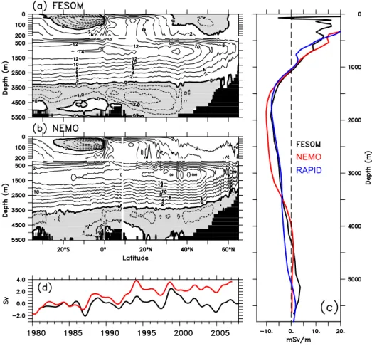
The AMOC is one of the most important quantities for the global overturning circulation, but often strongly differs among individual models even under similar atmospheric forcing (Danabasoglu et al., 2014). Small differences, in particular in the subpolar freshwater budget, can have important consequences on the strength, potentially leading to gradual trends (Behrens et al., 2013). Broadly, NEMO and FESOM share the similar general characteristics, with a North Atlantic Deepwater (NADW) cell on top of an AABW cell (Fig. 6). With 20 Sv, NEMO simulates a significantly stronger and deeper NADW cell than FESOM (14 Sv), which is to a certain part a result of the applied rain reduction north of 55°N in NEMO (Behrens et al., 2013). Probably as a result of the strong NADW cell, but also an effect of an insufficient downward spreading of AABW, NEMO shows a weaker AABW cell.

Compared to the transport from the observational RAPID array (Smeed et al., 2016), NEMO shows a good agreement in the upper 1500 m whereby FESOM strongly deviates in the upper 500 m. In the range of upper NADW (∼1000–3000 m), the southward transport in NEMO is too strong. Below, both simulations show the too weak pe- netration of the lower NADW, probably arising from an underrepresentation of the spreading of Denmark Strait overflow into the subpolar North Atlantic (Behrens et al., 2013). In respect of the temporal variability, both simulations confirm the good correlation (r = 0.72, significant at the 99% level,Fig. 6d) on interannual timescales which is consistent throughout the CORE intercomparison as a

result of the similar wind forcing (Danabasoglu et al., 2016). It is to note that both simulations show a direct wind-driven cell south of the equator, seen as a subtropical cell of similar strength (4–5 Sv) as a direct consequence of the (identical) wind forcing in the tropical Atlantic.

FESOM additionally shows an upper-ocean transport cell in the subtropical/subpolar North Atlantic, with near-surface southward transports up to 1 Sv between 35°N and 60°N. This has rarely seen among other models (Danabasoglu et al., 2014) and may have consequences for the exchange between the subpolar and subtropical gyres.

From the analysis of the large-scale circulation, we conclude that both conﬁgurations simulate a reasonable global circulation.

Differences arise from local horizontal grid resolution effects, the GM parameterization and specific numerical details impacting the formation and spreading of deep water masses.

4. Simulation of the Agulhas system

We now turn to the speciﬁc region of interest, the Agulhas system around South Africa. The Agulhas Current is the WBC of the Indian Ocean subtropical gyre and provides source waters for Agulhas leakage.

Simulating the correct structure and transport are therefore important prerequisites for a proper representation of the exchange processes south of Africa and theflow into the upper limb of the AMOC.Fig. 7 shows cross-sectional transports from moorings along the ‘Agulhas Current Time-series’(ACT) array (Beal et al., 2015) starting at the coast between Port Alfred and East London and following a southeast satellite track up to 300 km offthe coast (red lines inFig. 8b,c). Both simulations show the typical asymmetric profile of the southwardflowing Agulhas Current, with strongest speeds above the continental slope, up to 1.5 m s⁻¹in NEMO and 1.2 m s⁻¹in FESOM, compared to 1.7 m s⁻¹in the observations (Beal et al., 2015). FESOM shows a wider current of 250–300 km width (depending on whether a velocity isotach or the Fig. 2.Snapshots of speed (5-day average centered around 15 June 2006, in cm s⁻¹) at 50 m depth in (a) FESOM and (b) NEMO.

(6)

transport is taken), compared to about 219 km in the observations. If we take the 5-cm s⁻¹isotach as a criterion, depth and width of the current are quite realistically represented in NEMO. Despite the general good agreement in the structure, it is interesting to note that the transports in both simulations are oﬀby 10 Sv and more. For the traditional calculation of net transports over aﬁxed width, FESOM overestimates the transport due to its excessive width (Tbox; Table 1). Instead, NEMO underestimates the transport, probably because of the lower current speeds.

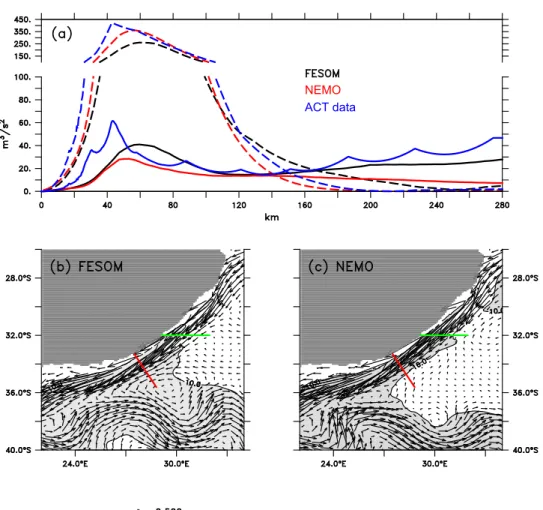
Beal et al. (2015) introduced a transport calculation following streamline approach to isolate the Agulhas Current transport from the short-term Natal Pulses.Beal and Elipot (2016)regressed the mooring transports onto SSH along the satellite track to derive a transport proxy over 22 years. If calculated accordingly, both simulations underestimate the transport (Tjet;Table 1). An explanation for the different ability to represent Tbox and Tjet can be seen in the distribution of mean and eddy transports across the section and a detailed distribution of currents: FESOM simulates a wider mean current (dashed curves in Fig. 8a), due to a prominent recirculation of flow from the Agulhas Return Current (Fig. 8b). This then leads to enhanced transports and a wider current profile compared to NEMO. Compared to the

observations, FESOM overestimates and NEMO underestimates the transport variability (both for Tbox and Tjet). The eddy kinetic energy profile also shows that both simulations underestimate the variability, in particular at the offshoreflank of the Agulhas Current (solid curves in Fig. 8a).

The strong nonlinear character of the WBC regime at the ACT section is representative of the southern Agulhas Current, that begins at

∼34°S with a widening of the shelf, in consequence providing less to- pographic steering. This nonlinearity leads to the fact that interannual transport variations are (despite the similar atmospheric forcing) un- correlated within the simulations or against ACT observations and proxy (Fig. 9). This is not surprising sinceBiastoch et al. (2009a)have shown that the interannual variability of the Agulhas Current is independent of the atmospheric forcing and rather a result of the short- term to mesoscale variability reflecting onto interannual timescales. Is the underrepresentation of transport in both simulations an important misfit? Since the wind forcing, hence Sverdrup contribution arising from the interior, is similar in both simulations, these differences come from the strength of recirculation (Fig. 8b,c). This is supported by a comparison with transport estimates at 32°S (green lines inFig. 8).

There, simulated Agulhas Currents have similar strengths (Table 1) and Fig. 3.Standard deviation of 5-daily sea surface height (in cm, 2000–2007) (a) FESOM, (b) NEMO and (c) AVISO.

(7)

are correlated on an interannual timescale (r = 0.6, signiﬁcant at the 99% level). The increase in transport variability between 32°S and the ACT section in FESOM hence is a result of the (nonlinear) recirculation in the direct vicinity of the WBC regime.

The net transport of the WBC, here derived from the streamfunction representing the net of the southwardflowing Agulhas Current and the northward flowing Agulhas Undercurrent (Fig. 9c), increases from north to south. The character of the increase is different in both simulations, with FESOM showing a strong increase in the southern Agulhas Current. Instead, NEMO simulates a more moderate and

uniform increase until 36°S; south of it, the transport strongly increases.

Interestingly, both simulations arrive at a similar transport of around 90 Sv at the southern end, correspond to the transport amplitude of the observations just few degrees southwest of the ACT section. We conclude that the mismatch between the simulations and with observations at the specific latitudes has less to do with the general architecture of the models but arises from numerics of the used advection or diffusion schemes. For example,Backeberg et al. (2009)showed that the choice of the advection scheme strongly determines the stability of the Agulhas Current. Loveday et al. (2014) demonstrated similar differences in Fig. 4.Horizontal transport streamfunction (in Sv, 1988–2007 mean) in (a) FESOM and (b) NEMO.

Table 1

Mean transports and standard deviations (Agulhas transports are based on 5-daily time series 1988–2007, others are derived from the monthly streamfunction 1958–2007, seeFig. 4). Observational estimates are from (1)Sprintall et al. (2009), (2)Ullgren et al. (2012), (3)Donohue et al. (2016), (4)Beal et al. (2015; in situ values at 5-daily resolution, lightblue inFig. 9), (5)Beal (2009; based on daily vaues). Agulhas transports are deﬁned as net transports over the mean width in each model (32°S) or consistent with the geometry and deﬁnition byBeal et al. (2015)(ACT). Agulhas Undercurrent transports are integrated from the northward velocities.

Natal Pulses are deﬁned as instances in which the 200 m maximum current is shifted oﬀshore by more than two std. dev. (6) The observational estimate is based on ACT in situ data and correspond toFig. 2a inElipot et al. (2015).

FESOM NEMO Observations

Indonesian Throughﬂow −13.0 ± 5.5 Sv −17.0 ± 3.5 Sv 15.0 Sv⁽¹⁾

Mozambique Channel −12.5 ± 6.9 Sv −17.8 ± 6.8 Sv 16.7 ± 15.8 Sv⁽²⁾

Drake Passage 149.5 ± 4.6 Sv 121.7 ± 6.1 Sv 173.3 Sv⁽³⁾

Agulhas Current (32°S) −61.9 ± 24.6 Sv −67.9 ± 19.3 Sv

Agulhas Current (ACT)–Tbox −82.5 ± 40.9 Sv −66.5 ± 18.8 Sv −77.5 ± 30.8 Sv⁽⁴⁾

Mean width 260 km 225 km 219 km⁽⁴⁾

–Tjet −74.9 ± 25.2 Sv −71.3 ± 16.2 Sv −83.8 ± 21.8 Sv⁽⁴⁾

Agulhas Undercurrent (ACT) 6.0 ± 9.2 Sv 5.9 ± 4.9 Sv 4.5 ± 5.2 Sv⁽⁵⁾

6.2 ± 5.6 Sv⁽⁴⁾

> 1000 m 5.1 ± 7.3 Sv 4.5 ± 4.1 Sv 2.3 ± 3.0 Sv⁽⁵⁾

3.7 ± 2.8 Sv⁽⁴⁾

Natal Pulses 1.6 year⁻¹ 1.4 year⁻¹ 1.4 year^{−1 (6)}

std. dev. 52 km 24 km 30 km

(8)

Agulhas Current transports among NEMO and ROMS models, both performed under similar atmospheric forcing.

Both simulations obtain a weak Agulhas Undercurrent of just 2 cm s⁻¹northwardflow, compared to observed 8–9 cm s⁻¹(Fig. 7). Their transports, however, compare well with observations (Table 1,Fig. 9), probably a result of a wider cross section. Both, Agulhas Current and Undercurrent are subject to a strong variability, the latter with standard deviations larger than the mean value. This is a result of the southward propagating Natal Pulses, steering the Agulhas Current offshore and leaving room for the Agulhas Undercurrent to reach up to the surface (Biastoch et al., 2009a). If we define Natal Pulses as instances in which the Agulhas Current is shifted offshore, both simulations produce surprisingly comparable numbers (Table 1) to the estimate by Elipot et al. (2015)for the in situ data, demonstrating that the formation and propagation mechanisms are realistically simulated. As noted earlier, in FESOM, however, the deviations through Natal Pulses are larger.

The detailed comparison of the Agulhas Current structure and transport demonstrates the challenge for OGCMs to match the correct transport number of observations in such a nonlinear WBC regime, given the reinforcement of transports through recirculations and the level of the mesoscale.

The Agulhas system is intensively studied because of its global re- levance. Most interesting is the quantification of how much of its original waters starting in the Agulhas Current arrive in the South Atlantic andflow into the upper branch of the AMOC. The exact amount of Agulhas leakage is the result of a complicated interplay between the retroflecting Agulhas Current and the nonlinear transport of surface and intermediate water through anticyclonic Agulhas rings, cyclonic eddies

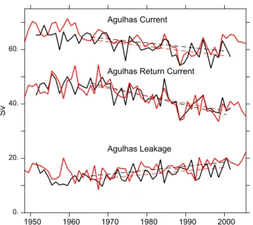
and direct inﬂow. For a quantiﬁcation of the individual drivers of the interoceanic exchange we use a Lagrangian estimate (Biastoch et al., 2008b; Durgadoo et al., 2013) that provides annual transport timeseries of the volumetric amount. For the calculation of the Lagrangian tra- jectories in the ARIANE software (Blanke et al., 1999), FESOM data were interpolated onto the NEMO grid. Before we study the fate of Agulhas Current waters, we will again focus on the transport of the Agulhas Current at 32°S (green lines in Fig. 8b,c), both simulations correspond to the similar atmospheric forcing with a comparable trend of −1.7 Sv decade⁻¹ in FESOM and −1.5 Sv decade⁻¹ in NEMO (Fig. 10).

The amount of Agulhas Current water arriving in the South Atlantic deﬁned by crossing of the Goodhope section (Ansorge et al., 2005), Agulhas leakage, also agrees surprisingly well with a mean of 14.5 Sv for FESOM and 16.1 Sv for NEMO (mean 1965–2000) and comparable annual standard deviations (2.2–2.3 Sv), demonstrating a similar relative portion of the retroﬂecting Agulhas Current. Although individual years do not match due to the dominance of upstream and downstream mesoscale vortices, both FESOM and NEMO follow the same behaviour:

Owing to the changes in Southern Hemisphere winds, decadal trends are similar. The trends towards stronger westerlies cause an increase of Agulhas leakage, with comparable values of 1.3 Sv decade⁻¹in FESOM and 1.5 Sv decade⁻¹in NEMO (Durgadoo et al., 2013). It is to note that this trend seems to be a swing in a multi-decadal variability (Biastoch et al., 2015). Corresponding to the increase in Agulhas leakage is a decrease of the Agulhas Return Current.

Can we assume that the reaction of Agulhas leakage to changing winds is similar in FESOM and NEMO?Durgadoo et al. (2013)used sensitivity experiments which artificially increase Southern Hemisphere Fig. 5.Interannually filtered transport timeseries through (a) Indonesian Archipelago, (b) Mozambique Channel and (c) Drake Passage (in Sv) for FESOM (black) and NEMO (red) as derived from the streamfunction (Fig. 4). (For interpretation of the references to colour in thisfigure legend, the reader is referred to the web version of this article.)

(9)

westerlies to study their impact on Agulhas leakage. They hypothesized that the response of the ACC to increased winds is an important factor inﬂuencing Agulhas leakage. With FESOM, we repeated the series of sensitivity experiments and artiﬁcially increased the westerlies by 40%

after year 30 in a climatologically forced reference experiment. Here,

the simulations show a different behaviour: As reported by Durgadoo et al. (2013), Agulhas leakage in NEMO initially increases by 38%, then collapses back to the reference state (Fig. 11;Table 2). In contrast, FESOM remains at an increased amount, reaches an even stronger level. The reason may be found in the response of the ACC Fig. 6.Atlantic meridional overturning streamfunction (in Sv, 1988–2007 mean) in (a) FESOM and (b) NEMO (calculated both for base and nest). Shaded in gray are anticlockwise (C.I. = 1 Sv), in white are clockwise (C.I. = 2 Sv) cells. Note that the vertical axis is split at 200 m. (c) Profiles of z-derivative of AMOC at 26.5°N for FESOM (black), NEMO (red) and RAPID observational data (2 April 2004–11 October 2015 mean, blue). (d) Timeseries of interannuallyfiltered AMOC anomaly at 26.5°N for FESOM (black) and NEMO (red). (For interpretation of the references to colour in thisfigure legend, the reader is referred to the web version of this article.)

Fig. 7.Western boundary current structure at the ACT line. Shown are 1988–2007 mean cross-section velocities (southwestward/negative shaded in white, northeastward/positive in grey, contoured are intervals of 1 cm s⁻¹in red, 5 cm s⁻¹in black and 10 cm s⁻¹in blue) for (a) FESOM, (b) NEMO and (c) ACT observations (1 May 2010–28 February 2013 mean). The green isoline shows the 5 cm s⁻¹from the observations. (For interpretation of the references to colour in thisﬁgure legend, the reader is referred to the web version of this article.)

(10)

south of Africa. While FESOM simulates an ACC, which is less than 10%

stronger than in the reference experiment, NEMO shows such a behaviour only in theﬁrst 10 years. Afterwards, the ACC strongly increases beyond 235 Sv. As a consequence, this reduces the Agulhas leakage back to its original value (Durgadoo et al., 2013). The increased ACC transport in NEMO is a result of stronger sloping isopycnals across the

ACC, mainly a result of the deeper convection and surfacing isopycnals south of the current (Farneti et al., 2015). Owing to an increased resolution but also the GM parameterization, an ACC increase due to the wind in FESOM seems to be compensated by mesoscale eddies. The strong impact of the ACC on Agulhas leakage points to the importance of remote impact of the large-scale circulation on the regional dynamics Fig. 8.(a) Vertically integrated mean (dashed) and eddy (solid) kinetic energy densities for FESOM (black) and NEMO (red) across the ACT section. The ACT in situ observations are shown in blue. Mean velocities (1988–2007, only every 5th in both directions shown, in m s⁻¹) for (b) FESOM and (C) NEMO. Shaded in light grey are eddy kinetic energy densities above 10 cm²s⁻². The lines mark the ACT (red) and 32°S (green) sections. (For interpretation of the references to colour in thisﬁgure legend, the reader is referred to the web version of this article.)

Fig. 9.Agulhas Current (southward, negative) and Agulhas Undercurrent (northward, positive) transports defined as (a) Tbox (for the models integrated up to the mean width, see Table 1) and (b) Tjet for FESOM (black), NEMO (red) and ACT in situ observations (lightblue) and proxy (blue). Note that the observational transport numbers inTable 1are based on the observations in 2010–2014. Shown in light colours are 5-daily transports, in bold interannual variations (monthly data with 23-month Hanningfilter). (c) Vertically integrated transports, derived from the minimum of the streamfunction (Fig. 4) within a coastal following strip to 250 km offthe 500- m isobath. Dashed lines represent the monthly std. dev. (For interpretation of the references to colour in thisfigure legend, the reader is referred to the web version of this article.)

(11)

around South Africa and the need to properly simulate the large-scale circulation away from the Agulhas system. This could be realized through a southward expansion of the nested region (NEMO) or by increasing the resolution over a larger area covered by the ACC (FESOM).

5. Numerical costs

In addition to the scientiﬁc quality described above, the numerical performance and costs determine the choice for a speciﬁc model.

Experiments with FESOM and NEMO (for a systematic evaluation of recent codes now in the actual NEMO version 3.6, but still in the INALT01 setup) were performed at a Cray XC40, equipped with Intel Xeon Haswell processors, of the North-German Supercomputing Alliance (‘Norddeutscher Verbund für Hoch- und Höchstleistungsrechnen’; HLRN).

Results for the total runtime per model year and with monthly outputﬁelds indicate a more performant NEMO code with 2–3 times lower CPU cost for the same runtime (Fig. 12a). Given the 2 times higher number of grid points in NEMO and 1.4 times higher number of operations (grid points x time steps for a given model year, for NEMO considering both base and nest), the runtime per grid point and time step is 1.5–2 times higher in FESOM (dotted curves in Fig. 12b).

However, FESOM has an impressive, nearly linear scalability. In NEMO, the base model subdomains get too small (< 20 grid points in both directions) to scale beyond 884 processors. This would be diﬀerent for a higher resolved base model (e.g. ORCA025 with 4 times more grid points compared to ORCA05). It shall also be noticed that FESOM does not calculate dry grid points (both land and bathymetry). The computational load in NEMO can be further reduced by blending out land processors which would be completely dry. This can make an additional 15% reduction in runtime. In FESOM, the bottleneck of eﬃciency is in memory access linked to how variables are allocated. It uses tetrahedral elements and one-dimensional arrays to store 3D variables. There is potential to speed up the code by re-structuring variable storage.

6. Summary and conclusion

In this study, we compared two global OGCMs, specifically set up to simulate the Agulhas system. The tasks for both configurations were (1) to simulate the intricacies of the mesoscale dynamics of the currents around South Africa, but also (2) to represent adequately the embedment within the global circulation. One configuration, based on NEMO, was set up in a traditional structured-mesh architecture and served as a widely analysed and well understood reference case. The one based on FESOM, using unstructured meshes, represents an approach that is Fig. 10.Agulhas Current (at 32°S, seeFig. 8) and Return Current and Agulhas leakage

estimated from Lagrangian methodology for FESOM (black) and NEMO (red). Dashed lines show the linear trends between 1965 and 2000. (For interpretation of the references to colour in thisﬁgure legend, the reader is referred to the web version of this article.)

Fig. 11.Transports for climatological (dashed) and increased westerlies (solid) experiments. Agulhas leakage for (a) FESOM and (b) NEMO. ACC (maximum streamfunction south of Africa between 20° and 30°E) for (c) FESOM and (d) NEMO.

(12)

relatively new for global ocean conﬁgurations, speciﬁcally at mesoscale resolution.

Both conﬁgurations represent the Agulhas system adequately.

Although each configuration shows typical deficits in comparison with observations, FESOM with a too wide Agulhas Current width and NEMO with a too weak transport, both do provide reasonable simulations to warrant scientific analyses and interpretations of the current system. Misfits to observations are especially seen in the southern Agulhas Current because of the strong nonlinearity and potential recirculations. Here, specific choices of numerical and physical schemes do alter the characteristics of the WBC regime. By changing the schemes within each model system, one could certainly easily span the range from a too narrow to a too wide current, from a too weak to a too high transport. The comparison shows that there is remarkable agreement of both configurations in respect to transports in the northern Agulhas Current, but also for the resulting WBC transport at the southern tip of Africa. In between, each configuration simulates a different latitudinal increase for which the amount of recirculation in the subgyre from the Agulhas Return Current into the Agulhas Current is important.

For Agulhas leakage, both configuration provide a surprisingly similar result, given the dominance of the nonlinearity for the retroflection and in the Cape Basin. Both configurations agree in respect to

the mean transport and decadal trends. Together with the interannual correlation in the northern Agulhas Current, the agreement in mean and trends in respect to Agulhas leakage conﬁrms the strong inﬂuence of the (identical) wind forcing for the integral measures of the Agulhas Current.

For the global circulation, which provides important boundary conditions of the openly set Agulhas system around South Africa, the situation is diﬀerent. Here, the unstructured-mesh approach can play out its advantages of a variable grid resolution where required. For the Southern Ocean, this leads to an improved representation of the density gradient across the ACC, and as a consequence to a more realistic ACC response to varying atmospheric boundary conditions. For the individual components of the AMOC, the path of the Gulf Stream or the exchange of water with the subpolar and subarctic North Atlantic, similar beneﬁts could play an important role for the proper interplay between Agulhas leakage and AMOC.

The conclusions above are consistent with the experiences gathered from the model assessment made under CORE forcing, even though these were performed at coarser resolutions. The circulation characteristics representing the wind-driven circulation, for example mean and decadal trends of dynamic sea level, are robust among a wide range of models under similar wind forcing (Griﬃes et al., 2014). In the Table 2

Transports and changes of Agulhas leakage (AL) and ACC transport (estimated as the maximum streamfunction south of Africa between 20°E and 30°E) in the reference and sensitivity experiments.

NEMO FESOM

CLIM SHW + 40% increase CLIM SHW + 40% increase

AL Years 35–40 15.7 Sv 21.8 Sv 38% 13.8 Sv 18.5 Sv 35%

Years 45–50 17.7 Sv 18.7 Sv 6% 13.1 Sv 20.9 Sv 59%

ACC Years 35–40 185 Sv 205 Sv 11% 188 Sv 199 Sv 6%

Years 45–50 181 Sv 235 Sv 30% 188 Sv 201 Sv 7%

Fig. 12.(a) Runtime (for one model year with monthly output) at a Cray XC40, (b) scaling (based on the smallest number of CPU in each conﬁguration) and runtime per grid point (GP) and time step (dotted lines, right axis) of FESOM (black) and NEMO (red). (For interpretation of the references to colour in thisﬁgure legend, the reader is referred to the web version of this article.)

(13)

Southern Ocean, where mesoscale eddies play an important role for the change of the ACC under changing westerlies (Farneti et al., 2010), resolution or eventually chosen eddy parameterizations are crucial and lead to a wider range of transports and responses even under the same forcing (Farneti et al., 2015). For the AMOC, the situation is even more complicated. Here, supposedly small changes in the model conﬁgura- tion irrespective of the horizontal resolution, make a big diﬀerence.

This is in particular true for the freshwater budget in the northern North Atlantic (Behrens et al., 2013) and the ability of the models to represent convection processes and the downslope flow of overflow water (Legg et al., 2006). Even under identical wind and thermohaline forcing, the resulting mean AMOC is quite different in strength and structure, even among configurations which arise from the similar model architectures (Danabasoglu et al., 2014). Instead, the good cor- respondence of the interannual AMOC variability is a somehow trivial result as it arises as a direct result from the identical wind forcing (Danabasoglu et al., 2016).

Despite the above-mentioned advantage of using multi-resolution unstructured-mesh models, certain eﬀorts are still required in the modelling community using such new generation models. Base models for the traditional structured-mesh approach are typically performed at distinct resolutions, usually 1/2° (ORCA05, this study) or 1/4°

(ORCA025,Böning et al., 2016). They are well understood in terms of strength and weaknesses of the simulated dynamics and hydrography, often tuned to provide a meaningful simulation for the given resolution because they are also run as standalone versions (see Biastoch et al. (2008)for ORCA05,Barnier et al. (2006)for ORCA025).

The unstructured-mesh approach instead has unlimited choices for the grid configuration. With the same purpose of setting up an Agulhas configuration, we could have set up a grid differing in resolution in the Drake Passage, along the WBC extensions or in deepwater formation regions in the subpolar North Atlantic. These could have then led to different responses in the large-scale circulation, and in consequence the embedment of the Agulhas system. In fact, when setting up FESOM for this specific enterprise, most of the initial discussions have been centred around the grid specifications. This then led to the definition of the grid following SSH standard deviation (Sein et al., 2016), in addition to some more uniform resolution around South Africa. This, however, puts most emphasis on the resolution of the mesoscale, leaves other regions such as narrow straits or key regions for the thermohaline circulation with large degrees of freedom and some uncertainty in respect to the expected simulation. An important lesson learned is certainly the importance of setting up a few well-tested, tuned and understood reference unstructured meshes, similar to the base models in the structured-mesh approach.

We are confident that the good agreement of results in the Agulhas system between unstructured and structures meshes are transferable to other regions, in particular to those where mesoscale processes interact with WBC and large-scale currents. For specific studies concentrating on one larger regime or on one ocean basin, structured meshes provide an optimal and efficient way to ensure uniform resolution throughout the region of interest. There, the nesting approach ensures a connection to the outside world ocean that is part of the simulation. In contrast, the use of a regional configuration often provides the risk that details in the open boundary conditions and the chosen boundary data may determine part of the solution (Herzfeld et al., 2011). Unstructured meshes will play out their advantage by providing a consistent representation of mesoscale dynamics in many key regions which shall be evenly represented in a global setup. However, the choice where to put high resolution is not trivial as we have seen in this Agulhas example.

An important factor for the choice of the numerical approach is the computational cost of the code, in particular runtime. If a researcher using unstructured meshes has to wait 1.5–2 times longer for a 60-year experiment that is typically executed in 10 days using a structured- mesh model, this may inﬂuence the decision. The good scalability of FESOM allows one to compensate the lower performance; however, this

requires additional computational costs. Vice versa, a structured-mesh model would allow a large number of (sensitivity) experiments with the same amount of computing resources. Alternatively, one could also invest part of the saved computing resource in an improved base model, such as the 1/4° ORCA025 with an improved representation of the mesoscale (Barnier et al., 2006). This would further minimise the difference in quality of the global circulation characteristics between the two modelling approaches.

The lack of performance in the unstructured-mesh approach may change in the future. New technologies applied in FESOM2 (Danilov et al., 2017) and other models using this numerical architecture (ICON,Korn, 2017; MPAS,Ringler et al., 2013) are based on prismatic elements. In this case, the neighbourhood information and coefficients used to compute horizontal derivatives becomes two-dimensional and related to all prisms below the given surface cell. With about 50 or more vertical layers used in present-day OGCMs the additional computational price of using unstructured-mesh infrastructure may become negligible, and the only real slowness factor is the slightly higher number offloating point operations in high-order transport al- gorithms. In fact, FESOM2 provides a speedup of about three times or better compared to the version used in this manuscript; it thus shows a performance comparable to that of a structured-mesh model. In the future, there is chance for a parity in the competition between the two technologies discussed here. Other issues, like those of effective resolution, parameterizations and user-friendliness will come into play.

We conclude that the unstructured-mesh approach is mature enough to provide realistic and meaningful model configurations, also in respect to mesoscale dynamics. The ability in specifying grid resolution outside the direct region of interest provides a bigflexibility. But it also requires a responsibility that the global circulation needs to be properly evaluated against observations and other model realisations, in particular in a few chosen reference configurations. Even without the gap in the computational costs between both architectures exists, traditional structured-grid models remain state-of-the-art for OGCM applications.

We believe that at the current stage, development promotion and usage of both types of models will help to advance model development and climate research in a long-term perspective.

Acknowledgments

This work received funding from German Federal Ministry of Education and Research (BMBF) under the research grants 03G0835A/

B and 03F0750A/B of the project SPACES-AGULHAS and the Helmholtz Association (J.V.D., grant IV014/GH018). Model experiments were performed at the North-German Supercomputing Alliance (HLRN) and at the High-Performance Center Stuttgart (HLRS). We acknowledge the availability of observational and proxy data from the ACT array (http://

act.rsmas.miami.edu) and from the RAPID-WATCH MOC monitoring project funded by the Natural Environment Research Council (http://

www.rapid.ac.uk/rapidmoc). The altimeter products were produced by Ssalto/Duacs and distributed by Aviso, with support from Cnes (http://

www.aviso.altimetry.fr/duacs). Data and visualization scripts to re- produce theﬁgures are available athttp://data.geomar.de. Jan Harlaß provided runtime numbers for the actual code version of NEMO. We thank Lisa Beal and Shane Elipot for comments on an earlier version of the manuscript. We thank Björn Backeberg and an anonymous reviewer for constructive comments in the review process

Supplementary materials

Supplementary material associated with this article can be found, in the online version, atdoi:10.1016/j.ocemod.2017.12.002.

References

Ansorge, I.J., Speich, S., Lutjeharms, J.R.E., Goni, G.J., Rautenbach, C.J.D.W., Froneman,