From Modal Logic to (Co)Algebraic Reasoning
Peter Padawitz, TU Dortmund, Germany July 25, 2021
(actual version: http://fldit-www.cs.tu-dortmund.de/∼peter/CTL.pdf)
Contents
1. Kripke models and modal formulas 5
2. Kripke models in Expander2 19
3. Model checking as simplification 28
modal 28
4. Model checking as term evaluation 33
5. Model checking as simplification 28
6. Specifications that import modal 37
micro 37
trans0 43
7. Model checking as data flow analysis 50
Examples 57
8. Acceptors and regular expressions 69
9. State equivalence and minimization 95
Examples 101
10. Simplifications 111
evaluate 114
base 123
11. (Co)resolution and (co)induction on (co)predicates 136
12. Man-wolf-goat-cabbage problem 142
13. Railway crossing 150
14. Mutual exclusion 161
15. N-queens problem 193
16. Robots 203
17. Filling problem 207
18. Elevator 214
19. Towers of Hanoi 215
20. Natural numbers 226
21. Lists 234
22. Streams 244
23. Binary trees 265
24. Lazy evaluation 278
25. Further examples 287
26. Beispiele aus [13] 288
27. Literatur 390
Kripke models and modal formulas
A Kripke model K = (Q, Lab, At, trans, transL, value, valueL) consists of
• a set Q of states,
• a set Lab of labels (actions, input, etc.),
• a set At of atoms,
• transition relations trans : Q → P (Q) and transL : Q × Lab → P (Q),
• value relations value : At → P (Q) and valueL : At × Lab → P (Q).
State and path formulas
are generated by the following CFG rules: Let S = {sf , pf } and V be an S-sorted set of variables.
sf → at | val(at, lab) for all at ∈ At
and lab ∈ Lab (1)
sf → true | false | ¬sf | sf ∨ sf | sf ∧ sf | sf ⇒ sf (2)
sf → EX sf | AX sf | hlabisf | [lab]sf for all lab ∈ L (4)
sf → x | µx.sf | νx.sf for all x ∈ V (5)
sf → EF sf | AF sf | EG sf | AG sf
sf → sf EU sf | sf AU sf | sf EW sf | sf AW sf sf → sf ER sf | sf AR sf
pf → at | at(lab) for all at ∈ At
and lab ∈ L (6) pf → true | false | ¬pf | pf ∨ pf | pf ∧ pf | pf ⇒ pf (7) pf → next pf | hlabipf | [lab]pf for all lab ∈ L (8)
pf → x | µx.pf | νx.pf for all x ∈ V (9)
pf → F pf | G pf | pf U pf | pf W pf | pf R pf
pf → pf ; pf
Assumptions
Both the local and global semantics of modal formulas defined below require that formulas resp. transition relations meet the following constraints:
• For every free variable x of a subformula ψ of a formula ϕ, ϕ encloses a smallest ab- straction µx.ϑ or νx.ϑ (see rules (5) and (9)) that encloses ψ.
= ⇒ Abstractions can be evaluated hierarchically.
• Every free occurrences of a variable x in µx.ϕ resp. νx.ϕ has positive polarity, i.e., the number of negation symbols of µx.ϕ resp. νx.ϕ above the occurrence is even.
= ⇒ All logical operators are monotone.
• → is image finite, i.e., for all q ∈ Q and lab ∈ Lab, trans(q ) and transL(lab)(q) are finite.
= ⇒ All logical operators are ω-bicontinuous.
= ⇒ Fixpoints can be computed incrementally as Kleene closures of the accompa-
nying step functions (see below).
Local semantics
The set of all paths of K
path(K) =
def{p ∈ Q
N| ∀ i ∈ N : p
i+1∈ trans(p
i)
∨ ∃ lab ∈ Lab : p
i+1∈ transL(p
i)(lab)
∨ (trans(p
i) = ∅ ∧
∀ lab ∈ Lab : transL(p
i)(lab) = ∅ ∧
∀ k > i : p
i= p
k)}
The set of all paths of K that start with q ∈ Q
path(K, q ) =
def{p ∈ path(K) | p
0= q}
Let q ∈ Q, at ∈ At, lab ∈ Lab, b : V → P (Q) and c : V → P (path(K )).
Validity of state formulas
q | = at ⇐⇒
defq ∈ value(at)
q | = at(lab) ⇐⇒
defq ∈ valueL(at, lab)
q | = true for all q ∈ Q ∪ path(K)
q | = false for no q ∈ Q ∪ path(K)
q | = ¬ϕ ⇐⇒
defq 6| = ϕ
q | = ϕ ∨ ψ ⇐⇒
defq | = ϕ or q | = ψ q | = ϕ ∧ ψ ⇐⇒
defq | = ϕ and q | = ψ q | = ϕ ⇒ ψ ⇐⇒
defq | = ¬ϕ ∨ ψ
q | = x ⇐⇒
defq ∈ b(x)
q | = µx.ϕ(x) ⇐⇒
defq ∈ least solution of x = ϕ(x) q | = νx.ϕ(x) ⇐⇒
defq ∈ greatest solution of x = ϕ(x) q | = EXϕ ⇐⇒
def∃ q
0∈ trans(q) : q
0| = ϕ
q | = AXϕ ⇐⇒
def∀ q
0∈ trans(q) : q
0| = ϕ
q | = hlabiϕ ⇐⇒
def∃ q
0∈ transL(q)(lab) : q
0| = ϕ q | = [lab]ϕ ⇐⇒
def∀ q
0∈ transL(q)(lab) : q
0| = ϕ q | = EF ϕ ⇐⇒
def∃ p ∈ path(K, q) ∃ i ∈ N : p
i| = ϕ q | = AF ϕ ⇐⇒
def∀ p ∈ path(K, q) ∃ i ∈ N : p
i| = ϕ q | = EGϕ ⇐⇒
def∃ p ∈ path(K, q) ∀ i ∈ N : p
i| = ϕ q | = AGϕ ⇐⇒
def∀ p ∈ path(K, q) ∀ i ∈ N : p
i| = ϕ
q | = ϕ EU ψ ⇐⇒
def∃ p ∈ path(K, q) ∃ i ∈ N : p
i| = ψ ∧ ∀ j < i : p
j| = ϕ
q | = ϕ AU ψ ⇐⇒
def∀ p ∈ path(K, q) ∃ i ∈ N : p
i| = ψ ∧ ∀ j < i : p
j| = ϕ
q | = ϕ EW ψ ⇐⇒
def∃ p ∈ path(K, q) ∀ i ∈ N : p
i| = ψ ⇒ ∀ j < i : p
j| = ϕ q | = ϕ AW ψ ⇐⇒
def∀ p ∈ path(K, q) ∀ i ∈ N : p
i| = ψ ⇒ ∀ j < i : p
j| = ϕ q | = ϕ ER ψ ⇐⇒
def∃ p ∈ path(K, q) ∀ i ∈ N : p
i| = ψ ∨ ∃ j < i : p
j| = ϕ q | = ϕ AR ψ ⇐⇒
def∀ p ∈ path(K, q) ∀ i ∈ N : p
i| = ψ ∨ ∃ j < i : p
j| = ϕ
EF phi
phi
AG phi phi
phi
phi
phi phi
phi
phi
phi phi phi
EG phi phi
phi
phi
AF phi
phi phi
phi phi phi
phi EU psi phi
phi
phi
psi
phi AU psi phi
phi
phi
psi phi
psi
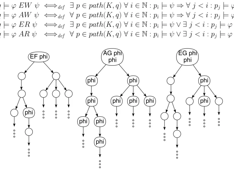
Fig. 1. Transition graphs whose roots satisfy EF ϕ, AGϕ and EGϕ, respectively
10
EF phi
phi
AG phi phi
phi
phi
phi phi
phi
phi
phi phi phi
EG phi phi
phi
phi
AF phi
phi phi
phi phi phi
phi EU psi phi
phi
phi
psi
phi AU psi phi
phi
phi
psi phi
psi
psi
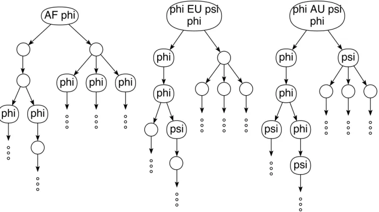
Fig. 2. Transition graphs whose roots satisfy AF ϕ, ϕEU ψ and ϕAU ψ, respectively
Validity of path formulas
p | = at ⇐⇒
defp
0∈ value(at)
p | = at(lab) ⇐⇒
defp
0∈ valueL(at, lab) p | = true for all p ∈ S ∪ path(K ) p | = false for no p ∈ S ∪ path(K) p | = ¬ϕ ⇐⇒
defp 6| = ϕ
p | = ϕ ∨ ψ ⇐⇒
defp | = ϕ oder q | = ψ p | = ϕ ∧ ψ ⇐⇒
defp | = ϕ und q | = ψ p | = ϕ ⇒ ψ ⇐⇒
defp | = ¬ϕ ∨ ψ
p | = x ⇐⇒
defs ∈ c(x)
p | = µxϕ ⇐⇒
defp ∈ least solution in x of the equation x = ϕ p | = νxϕ ⇐⇒
defp ∈ greatest solution in x of the equation x = ϕ p | = nextϕ ⇐⇒
defλi.p
i+1| = ϕ
p | = F ϕ ⇐⇒
def∃ i ∈ N : λk.p
i+k| = ϕ p | = Gϕ ⇐⇒
def∀ i ∈ N : λk.p
i+k| = ϕ
p | = ϕ U ψ ⇐⇒
def∃ i ∈ N : λk.p
i+k| = ψ ∧ ∀ j < i : λk.p
j+k| = ϕ
p | = ϕ W ψ ⇐⇒
def∀ i ∈ N : λk.p
i+k| = ψ ⇒ ∀ j < i : λk.p
j+k| = ϕ
p | = ϕ R ψ ⇐⇒
def∀ i ∈ N : λk.p
i+k| = ψ ∨ ∃ j < i : λk.p
j+k| = ϕ
p | = ϕ ; ψ ⇐⇒
defp | = G(ϕ ⇒ F ψ)
Global semantics
The abstract syntax of the above grammar generating state and path formulas – except rules (5) and (9) – is given by a constructive signature Σ = (S, OP ) with sort set S = {sf , pf }.
The sf - or pf -constructors of Σ are usually called modal or temporal operators, respectively.
Every state or path formula is represented by a Σ-term over V .
The global semantics of state and path formulas is given by the following Σ-Algebra A = (A, Op) (see [18]):
A
sf= P (Q)
A
pf= P (path(K))
For all qs, qs
0⊆ Q and f : Q → P (Q),
imgsShares(qs)(f )(qs
0) =
def{q ∈ qs | f (q) ∩ qs
06= ∅}, imgsSubset(qs)(f )(qs
0) =
def{q ∈ qs | f (q) ⊆ qs
0}.
For all at ∈ At, lab ∈ Lab, qs, qs
0⊆ Q and ps, ps
0⊆ path(K), at
A= value(at)
at(lab)
A= valueL(at, lab)
true
A= Q false
A= ∅
¬
A(qs) = Q \ qs
∨
A= ∪
∧
A= ∩
qs ⇒
Aqs
0= (Q \ qs) ∪ qs
0EX
A= imgsShares(Q)(trans) AX
A= imgsSubset(Q)(trans)
hlabi
A= imgsShares(Q)(flip(transL)(lab)) [lab]
A= imgsSubset(Q)(flip(transL)(lab)) true
A= path(K)
¬
A(ps) = path(K) \ ps
ps ⇒
Aps
0= (path(K ) \ ps) ∪ ps
0next
A(ps) = {p ∈ path(K ) | λi.p
i+1∈ ps}
flip : (a → b → c) → (b → a → c) denotes the Haskell function that exchanges the
arguments of a cascaded binary function.
The remaining modal and temporal operators are reduced to µ- resp. ν -abstractions:
EF ϕ = µx.ϕ ∨ EX x
AF ϕ = µx.ϕ ∨ (AX x ∧ EX true) EGϕ = νx.ϕ ∧ (EX x ∨ AX false ) AGϕ = νx.ϕ ∧ AX x
ϕ EU ψ = µx.ψ ∨ (ϕ ∧ EX x) ϕ AU ψ = µx.ψ ∨ (ϕ ∧ AX x) ϕ EW ψ = νx.ψ ∨ (ϕ ∧ EX x) ϕ AW ψ = νx.ψ ∨ (ϕ ∧ AX x) ϕ ER ψ = νx.ψ ∧ (ϕ ∨ EX x) ϕ AR ψ = νx.ψ ∧ (ϕ ∨ AX x) F ϕ = µx.ϕ ∨ next x
Gϕ = νx.ϕ ∧ next x
ϕ U ψ = µx.ψ ∨ (ϕ ∧ next x) ϕ W ψ = νx.ψ ∨ (ϕ ∧ next x) ϕ R ψ = νx.ψ ∧ (ϕ ∨ next x) ϕ ; ψ = G(ϕ ⇒ F ψ )
Σ-terms representing µ- or ν -abstractions are evaluated in A as follows:
Since A
sfand A
pfare powersets and thus ω-bicomplete carrier sets – with partial order ⊆, least element ∅ and greatest element Q resp. path(K) (see [18]) –, Kleene’s Fixpoint Theorem (see [12, 18]) provides us with the least fixpoint
lfp (f ) = G
n∈N
f
n(false
A) and the greatest fixpoint
gfp (f ) = l
n∈N
f
n(true
A)
of every S-sorted ω-bicontinuous function f : A → A.
If A
sfund A
pfare finite, then
lfp (f ) = fixpt (≤)(f )(false
A) and gfp (f ) = fixpt (≥)(f )(true
A) where
fixpt : (A → A → Bool) → (A → A) → (A → A) is defined as follows:
fixpt (≤)(f )(a) = if f (a) ≤ a then a else fixpt (≤)(f )(f (a))
Let ϕ be a modal formula satisfying the above assumptions and g : V → A be an S -sorted
function.
The extension g
∗: T
Σ(V ) → A of g to Σ-terms is inductively defined as follows:
For all x ∈ V , s ∈ {sf , pf }, op : s
n→ s ∈ OP , ϕ
1, . . . , ϕ
n∈ T
Σ(V )
sand ϕ ∈ T
Σ(V ),
g
∗(x) = g(x),
g
∗(op(ϕ
1, . . . , ϕ
n)) = op
A(g
∗(ϕ
1), . . . , g
∗(ϕ
n)), g
∗(µx.ϕ) = lfp (λa.g[a/x]
∗(ϕ)), (1) g
∗(νx.ϕ) = gfp (λa.g[a/x]
∗(ϕ)). (2)
Under the above assumptions on formulas and transition relations, the function λa.g[a/x]
∗(ϕ) : A → A
is ω-bicontinuous and thus (1) is the least and (2) the greatest fixpoint of λa.g [a/x]
∗(ϕ).
Two formulas ϕ and ψ are A-equivalent, written: ϕ ∼ ψ, if for all g : V → A,
g
∗(ϕ) = g
∗(ψ).
For instance,
¬F ϕ ∼ G(¬ϕ)
¬(ϕ R ψ) ∼ ¬ϕ U ¬ψ
F ϕ ∼ true U ϕ
Gϕ ∼ ϕ W false
ϕ U ψ ∼ (ϕ W ψ) ∧ F ψ ϕ W ψ ∼ (ϕ U ψ ) ∨ Gϕ
In the following chapters 3 to 7 we only deal with state formulas. Path formulas (and
temporal logic) are treated in chapter 22 in the context of the specification stream.
Kripke models in Expander2
The command specification > build Kripke model constructs a Kripke model K = (Q, At, Lab, trans, transL, value, valueL)
from parts of the actual specification SP . The sets Q, At and Lab are stored in the constants
states, atoms, labels :: [Term String]
where Term String is the String-instance of the datatype
data Term a = V a | F a [Term a] | Hidden Special type TermS = Term String
leaf a = F a []
SP should contain an axiom states == inits where inits evaluates to a list of initial states. build Kripke model adds to states all states that are reachable from inits via the transition axioms of SP , which have the following form:
ϕ ==> st -> st’ , ϕ ==> st -> branch$sts ,
ϕ ==> (st,lab) -> st’, ϕ ==> (st,lab) -> branch$sts
st, lab, st’ and sts are supposed to evaluate to a state or atom, a label, a state or a list of states, respectively.
The transition axioms of SP are converted into the transition and value relations of K and stored as the lists
trans, value :: [[Int]]
transL, valueL :: [[[Int]]]
such that for all i, j, k ∈ N ,
i ∈ trans!!j ⇐⇒ states!!i ∈ trans(states!!j ),
i ∈ transL!!j !!k ⇐⇒ states!!i ∈ transL(states!!j )(labels!!k), i ∈ value!!j ⇐⇒ atoms!!i ∈ value(atoms!!j ),
i ∈ valueL!!j !!k ⇐⇒ atoms!!i ∈ valueL(atoms!!j )(labels!!k).
Signatures in Expander2 (see Eterm.hs)
Symbols, simplification axioms and transition axioms are stored in the signature of SP that
is an object of the following O’Haskell type.
struct Sig = isPred,isCopred,isConstruct,isDefunct,isFovar,isHovar,blocked :: String -> Bool
hovarRel :: String -> String -> Bool
simpls,transitions :: [(Term String,[Term String],Term String)]
states,atoms,labels :: [Term String]
trans,value :: [[Int]]
transL,valueL :: [[[Int]]]
safeEqs :: Bool
out,parents :: Sig -> [[Int]]
out sig = invertRel sig.atoms sig.states sig.value parents sig = invertRel sig.states sig.states sig.trans invertRel :: [a] -> [b] -> [[Int]] -> [[Int]]
invertRel as bs iss = map f $ indices_ bs where f i = searchAll (i `elem`) iss outL,parentsL :: Sig -> [[[Int]]]
outL sig = invertRelL sig.labels sig.atoms sig.states sig.valueL parentsL sig = invertRelL sig.labels sig.states sig.states sig.transL invertRelL :: [a] -> [b] -> [c] -> [[[Int]]] -> [[[Int]]]
invertRelL as bs cs isss = map f $ indices_ cs
where f i = map g [0..length as-1] where
where g j = searchAll h isss where h iss = i `elem` iss!!j
Commands of the solver template (see Ecom.hs) access components of the current signature via the following command:
getSignature = do
let (ps,cps,cs,ds,fs,hs) = symbols
(sts,ats,labs,tr,trL,va,vaL) = kripke
isPred = (`elem` ps) ||| projection isCopred = (`elem` cps) ||| projection
isConstruct = (`elem` cs) ||| just . parse int |||
just . parse real ||| just . parse quoted |||
just . parse (strNat "inj") isDefunct = (`elem` ds) ||| projection isFovar = shares [x,base x] fs
isHovar = shares [x,base x] $ map fst hs hovarRel x y = isHovar x &&
case lookup (base x) hs of
Just es@(_:_) -> isHovar y || y `elem` es _ -> not $ isFovar y
(block,xs) = constraints
blocked x = if block then z `elem` xs else z `notElem` xs where z = head $ words x
simpls = simplRules; transitions = transRules
states = sts; atoms = ats; labels = labs; trans = tr transL = trL; value = va; valueL = vaL; safeEqs = safe;
return $ struct ..Sig
projection :: String -> Bool
projection = just . parse (strNat "get")
Embedding of trans, transL, out and outL into the simplifier
mkStates,mkLabels,mkAtoms :: Sig -> [Int] -> TermS mkStates sig = mkList . map (sig.states!!)
mkLabels sig = mkList . map (sig.labels!!) mkAtoms sig = mkList . map (sig.atoms!!) simplifyS sig (F "trans" state@(_:_)) =
if null sig.states then Just $ mkList $ simplReducts sig True st else do i <- search (== st) sig.states
Just $ mkStates sig $ sig.trans!!i where st = mkTup state
simplifyS sig (F "$" [F "transL" state@(_:_),lab]) =
if null sig.states then Just $ mkList $ simplReducts sig True
$ mkPair st lab else do i <- search (== st) sig.states
k <- search (== lab) sig.labels
Just $ mkStates sig $ sig.transL!!i!!k where st = mkTup state
simplifyS sig (F "out" state@(_:_)) =
if null sig.states then Just $ mkList $ filter f sig.atoms else do i <- search (== st) sig.states
Just $ mkAtoms sig $ out sig!!i where st = mkTup state
f = elem st . simplReducts sig True simplifyS sig (F "$" [F "outL" state@(_:_),lab]) =
if null sig.states then Just $ mkList $ filter f sig.atoms else do i <- search (== st) sig.states
k <- search (== lab) sig.labels Just $ mkAtoms sig $ outL sig!!i!!k where st = mkTup state
f = elem (mkPair st lab) . simplReducts sig True
Further functions for analyzing the Kripke model stored in the actual signature All successors of state
simplifyS sig (F "succs" state) = do i <- search (== st) sig.states
Just $ mkStates sig $ fixpt subset f [i]
where st = mkTup state
f is = is `join` joinMap g is ks = indices_ sig.labels
g i = sig.trans!!i `join`
joinMap ((sig.transL!!i)!!) ks
Direct predessors of state
simplifyS sig (F "parents" state) = do i <- search (== st) sig.states
Just $ mkStates sig $ parents sig!!i where st = mkTup state
simplifyS sig (F "$" [F "parentsL" state,lab])
= do i <- search (== st) sig.states k <- search (== lab) sig.labels
Just $ mkStates sig $ parentsL sig!!i!!k where st = mkTup state
All predecessors of state
simplifyS sig (F "preds" state) = do i <- search (== st) sig.states
Just $ mkStates sig $ fixpt subset f [i]
where st = mkTup state
f is = is `join` joinMap g is ks = indices_ sig.labels
g i = parents sig !!i `join`
joinMap ((parentsL sig!!i)!!) ks
All state/label sequences from state1 to state2
simplifyS sig (F "$" [F "traces" state,st']) =
do i <- search (== st) sig.states j <- search (== st') sig.states
jList $ map (mkStates sig) $ traces f i j where st = mkTup state
ks = indices_ sig.labels f i = sig.trans!!i `join`
joinMap ((sig.transL!!i)!!) ks simplifyS sig (F "$" [F "tracesL" state,st']) =
do i <- search (== st) sig.states j <- search (== st') sig.states
jList $ map (mkLabels sig) $ tracesL ks f i j where st = mkTup state
ks = indices_ sig.labels f i k = (sig.transL!!i)!!k traces :: Eq a => (a -> [a]) -> a -> a -> [[a]]
traces f a = h [a] a where
h visited a c = if a == c then [[a]]
else do b <- f a`minus`visited trace <- h (b:visited) b c [a:trace]
tracesL :: Eq a => [lab] -> (a -> lab -> [a]) -> a -> a -> [[lab]]
tracesL labs f a = h [a] a where
h visited a c = if a == c then [[]]
else do lab <- labs
b <- f a lab`minus`visited trace <- h (b:visited) b c [lab:trace]
Model checking as simplification
The following specification provides
• simplification axioms for reducing modal operators such that they can be evaluated in ctlAlg with eval/G (see above),
• simplification axioms for reducing state or path formulas to True or False,
• (co-)Horn clauses for proving state or path formulas by (co)resolution.
The constant noProcs is set by pressing the specification > set number of processes button.
modal
defuncts: noProcs procs states labels atoms valid
preds: X sat satL -> true false not \/ /\ `then` or and alloutL allanytrans allanytransL EX XE <> >< EF AF FE FA `EU` `AU`
copreds: ~ eqstate AX XA # ## AG EG GE GA `EW` `AW` `ER` `AR`
fovars: s s' st st' lab at hovars: X
axioms:
procs == [0..noProcs-1] -- used in many specifications that import modal -- state equivalence relations
& (eqstate <==> NU X.rel((st,st'),out$st=out$st' &
alloutL(st,st') &
allanytrans(X)(st,st') &
allanytrans(X)(st',st) &
allanytransL(X)(st,st') &
allanytransL(X)(st',st)))
& (st ~ st' ===> out$st=out$st' &
alloutL(st,st') &
allanytrans(~)(st,st') & allanytrans(~)(st',st) &
allanytransL(~)(st,st') & allanytransL(~)(st',st))
& (alloutL(st,st') <==> all(rel(lab,outL(st)$lab=outL(st')$lab))$labels)
& (allanytrans(P)(st,st') <==> allany(P)(trans$st,trans$st'))
& (allanytransL(P)(st,st') <==> all(rel(lab,allany(P)(transL(st)$lab, transL(st')$lab)))
$labels) -- simplification of first-order state formulas
& (sat(at)$st <==> at `in` out$st)
& (satL(at,lab)$st <==> at `in` outL(st)$lab)
& (EX(P)$st <==> any(P)$concat$trans(st):map(transL$st)$labels)
& (AX(P)$st <==> all(P)$concat$trans(st):map(transL$st)$labels)
& ((lab<>P)$st <==> any(P)$transL(st)$lab)
& ((lab#P)$st <==> all(P)$transL(st)$lab)
& (XE(P)$st <==> any(P)$parents$st)
& (XA(P)$st <==> all(P)$parents$st)
& ((lab><P)$st <==> any(P)$parentsL(st)$lab)
& ((lab##P)$st <==> all(P)$parentsL(st)$lab)
& (true$st <==> True)
& (false$st <==> False)
& (not(P)$st <==> Not(P$st))
& ((P/\Q)$st <==> P$st & Q$st)
& ((P\/Q)$st <==> P$st | Q$st)
& ((P`then`Q)$st <==> (P$st ==> Q$st))
-- simplification of second-order state formulas
& (or <==> foldl(\/)$false)
& (and <==> foldl(/\)$true)
& (EF$P <==> MU X.(P\/EX$X)) -- forward finally on some path
& (FE$P <==> MU X.(P\/XE$X)) -- backwards finally on some path
& (AF$P <==> MU X.(P\/(AX(X)/\EX$true))) -- forward finally on all paths
& (FA$P <==> MU X.(P\/(XA(X)/\XE$true))) -- backwards finally on all paths
& (EG$P <==> NU X.(P/\(EX(X)\/AX$false))) -- forward generally on some path
& (GE$P <==> NU X.(P/\(XE(X)\/XA$false))) -- backwards generally on some path
& (AG$P <==> NU X.(P/\AX$X)) -- forward generally on all paths
& (GA$P <==> NU X.(P/\XA$X)) -- backwards generally on all paths
& ((P`EU`Q) <==> MU X.(Q\/(P/\EX$X))) -- until
& ((P`AU`Q) <==> MU X.(Q\/(P/\AX$X)))
& ((P`EW`Q) <==> NU X.(Q\/(P/\EX$X))) -- weak until
& ((P`AW`Q) <==> NU X.(Q\/(P/\AX$X)))
& ((P`ER`Q) <==> NU X.(Q/\(P\/EX$X))) -- release
& ((P`AR`Q) <==> NU X.(Q/\(P\/AX$X))) -- narrowing of first-order state formulas
& (EF(P)$st <=== P$st | EX(EF$P)$st) -- forward finally on some path
& (AG(P)$st ===> P$st & AX(AG$P)$st) -- forward generally on all paths
& (AF(P)$st <=== P$st | AX(AF$P)$st & EX(true)$st)
-- forward finally on all paths
& (EG(P)$st ===> P$st & (EX(EG$P)$st | AX(false)$st))
-- forward generally on some path
& (FE(P)$st <=== P$st | XE(FE$P)$st) -- backwards finally on some path
& (GA(P)$st ===> P$st & XA(GA$P)$st) -- backwards generally on all paths
& (FA(P)$st <=== P$st | XA(FA$P)$st & XE(true)$st)
-- backwards finally on all paths
& (GE(P)$st ===> P$st & (XE(GE$P)$st | XA(false)$st))
-- backwards generally on some path
& ((P`EU`Q)$st <=== Q$st | P$st & EX(P`EU`Q)$st) -- until
& ((P`AU`Q)$st <=== Q$st | P$st & AX(P`AU`Q)$st)
& ((P`EW`Q)$st ===> Q$st | P$st & EX(P`EW`Q)$st) -- weak until
& ((P`AW`Q)$st ===> Q$st | P$st & AX(P`AW`Q)$st)
& ((P`ER`Q)$st ===> Q$st & (P$st | EX(P`ER`Q)$st)) -- release
& ((P`AR`Q)$st ===> Q$st & (P$st | AX(P`AR`Q)$st))
Model checking as term evaluation
Given the representation of a Kripke model K produced by build Kripke model (see chapte 2), the following Haskell code implements the global semantics of state formulas w.r.t. K (see chapter 1).
A signature for state formulas
struct Modal a label = true,false :: a neg :: a -> a
or,and :: a -> a -> a ex,ax,xe,xa :: a -> a
dia,box,aid,xob :: label -> a -> a The Modal-algebra of state sets
ctlAlg :: Sig -> Modal [Int] Int ctlAlg sig = struct true = sts
false = []
neg = minus sts or = join
and = meet
ex = imgsShares sts $ f sig.trans sig.transL ax = imgsSubset sts $ f sig.trans sig.transL
xe = imgsShares sts $ f (parents sig) (parentsL sig) xa = imgsSubset sts $ f (parents sig) (parentsL sig)
box = imgsSubset sts . flip (g sig.transL) aid = imgsShares sts . flip (g $ parentsL sig) xob = imgsSubset sts . flip (g $ parentsL sig) where sts = indices_ sig.states
f trans transL i = join (trans!!i) $ joinMap (g transL i)
$ indices_ sig.labels g transL i k = transL!!i!!k
The interpreter of state formulas in ctlAlg
type States = Maybe [Int]
foldModal :: Sig -> TermS -> States foldModal sig = f $ const Nothing where
alg = ctlAlg sig
f :: (String -> States) -> TermS -> States f g (F x []) | just a = a where a = g x f _ (F "true" []) = Just alg.true f _ (F "false" []) = Just alg.false
f g (F "not" [t]) = do a <- f g t; Just $ alg.neg a f g (F "\\/" [t,u]) = do a <- f g t; b <- f g u
Just $ alg.or a b
f g (F "/\\" [t,u]) = do a <- f g t; b <- f g u Just $ alg.and a b f g (F "`then`" [t,u]) = do a <- f g t; b <- f g u
Just $ alg.or (alg.neg a) b
f g (F "EX" [t]) = do a <- f g t; Just $ alg.ex a f g (F "AX" [t]) = do a <- f g t; Just $ alg.ax a f g (F "XE" [t]) = do a <- f g t; Just $ alg.xe a f g (F "XA" [t]) = do a <- f g t; Just $ alg.xa a f g (F "<>" [lab,t]) = do a <- f g t; k <- searchL lab
Just $ alg.dia k a
f g (F "#" [lab,t]) = do a <- f g t; k <- searchL lab Just $ alg.box k a
f g (F "><" [lab,t]) = do a <- f g t; k <- searchL lab Just $ alg.aid k a
f g (F "##" [lab,t]) = do a <- f g t; k <- searchL lab Just $ alg.xob k a
f g (F ('M':'U':' ':x) [t]) = fixptM subset (step g x t) alg.false f g (F ('N':'U':' ':x) [t]) = fixptM supset (step g x t) alg.true f _ (F "$" [at,lab]) = do i <- searchA at; k <- searchL lab
Just $ sig.valueL!!i!!k
f _ at = do i <- searchA at; Just $ sig.value!!i searchA,searchL :: Term String -> Maybe Int
searchA at = search (== at) sig.atoms searchL lab = search (== lab) sig.labels
step :: (String -> States) -> String -> TermS -> [Int] -> States step g x t a = f (upd g x $ Just a) t
f(g) :: Term String -> Maybe [Int] implements the (modal part of the) extension g
∗: T
Σ(V ) → A (see Kripke models in Expander2).
Embedding of foldModal(sig) into the simplifier
eval(ϕ) ϕ
AevalG(ϕ)
transition graph of K with all q ∈ ϕ
Acolored green
simplifyS (F "eval" [phi]) sig = do sts <- foldModal sig phi Just $ mkStates sig sts simplifyS (F "evalG" [phi]) sig = do sts <- foldModal sig phi
let f st = if st `elem` map (strs!!) sts then "dark green$"++st else st Just $ mapT f $ eqsToGraph [] eqs
where [strs,labs] = map (map showTerm0)[sig.states,sig.labels]
(eqs,_) = if null labs then relToEqs 0 $ mkPairs strs strs sig.trans else relLToEqs 0 $ mkTriples strs labs strs sig.transL
Specifications that import modal
Actions for building and verifying a specification involving a Kripke model
◦ enter the name of the specification into the entry field
◦ press the return key: the specification is parsed
◦ press the specification > build Kripke model button
A Kripke model is constructed from axioms of the specification
◦ press graph > show graph of Kripke model > here, and a graph comprising the states, atoms and transitions of the Kripke model is displayed on the solver canvas
◦ press paint, and the graph is displayed on the painter canvas (see below)
◦ customize the graph structure by moving nodes and red arc support points
◦ press combis, and the red arc support points are removed
micro (see [3], section 4.1)
specs: modal
constructs: start close heat error axioms:
states == [1] -- initial sates
& atoms == [start,close,heat,error]
& 1 -> branch[2,3] & 2 -> 5 & 3 -> branch[1,6]
& 4 -> branch[1,3,4] & 5 -> branch[2,3] & 6 -> 7 & 7 -> 4
& start -> branch[2,5,6,7]
& close -> branch[3..7]
& heat -> branch[4,7]
& error -> branch[2,5]
conjects: -- proof files
EF(Sat$heat)$5 --> True micro1P
& EG(Sat$heat)$7 --> True micro2P, micro2cycleP
& AF(Sat$heat)$6 --> True (16 parallel simplifications)
& all(EF$Sat$heat)$states --> True micro3P
& all(AF$Sat$heat)[4,6,7] --> True (26 parallel simplifications) terms:
eval$EF$heat --> states
<+> eval$EG$heat --> [4,7]
<+> eval$AF$heat --> [4,6,7]
<+> eval$start`then`heat --> [1,3,4,7]
<+> eval$EX$start`then`heat --> [1,3,4,5,6,7]
<+> eval$error`then`AG$not$heat --> [1,3,4,6,7]
After the above actions the following graph appears on the painter canvas:
1
2:[start,error]
5:[start,close,error]
3:close
6:[start,close]
7:[start,close,heat]
4:[close,heat]
Four of the five conjectures of micro can be proved by applying simplification axioms and selection > permute subtrees. Due to the fact that the second conjecture involves the greatest fixpoint EG (see modal ) is led into a cycle with simplification and subtree permutation (see micro2cycleP ). Applying selection > coinduction, however, leads to a successful proof (see micro2P). It contains two coinduction steps because EG(Sat$heat)$7 can only be shown along with EG(Sat$heat)$4 (see chapter 9 below or [18], chapter 17).
Here is the proof as recorded by Expander2 in micro2P:
0. Derivation of EG(Sat(heat))$7
All simplifications are admitted.
Equation removal is safe.
1. Adding
(EG0(z0)$z1 <=== z0 = Sat(heat) & z1 = 7) to the axioms and applying COINDUCTION wrt
(EG(P)$st ===> P(st) & (EX(EG(P))$st | AX(false)$st)) at positions [] of the preceding trees leads to
EG0(Sat(heat))$4
The reducts have been simplified in parallel.
2. Adding
(EG0(z2)$z3 <=== z2 = Sat(heat) & z3 = 4) to the axioms and applying COINDUCTION wrt
(EG(P)$st ===> P(st) & (EX(EG(P))$st | AX(false)$st)) at positions [] of the preceding trees leads to
EG0(Sat(heat))$1 | EG0(Sat(heat))$3 | EG0(Sat(heat))$4 The reducts have been simplified in parallel.
3. NARROWING the preceding trees (one step) leads to EG0(Sat(heat))$3 | EG0(Sat(heat))$4
The axioms have been MATCHED against their redices.
The reducts have been simplified in parallel.
4. NARROWING the preceding trees (one step) leads to EG0(Sat(heat))$4
The axioms have been MATCHED against their redices.
The reducts have been simplified in parallel.
The formula coincides with no. 1
5. NARROWING the preceding trees (one step) leads to True
The axioms have been MATCHED against their redices.
The reducts have been simplified in parallel.
trans0
specs: modal
constructs: is less defuncts: drawI drawS axioms:
states == [0,22]
& atoms == map($)$prodL[[is,less],states]
& (st < 6 ==> st -> st+1<+>ite(st`mod`2 = 0,st,()))
& 6 -> branch$[1..5]++[7..10]
& 7 -> 14
& 22 -> 33<+>44
& is$st -> st
& less$st -> valid(<st) -- widget interpreters:
& drawI == wtree $ fun(st,ite(st`in`states,
color(index(st,states),length$states)$circ$11, frame(3)$blue$text$st))
conjects:
(=14)$3 --> False
& AG(<14)$9 --> True
& all(EX(=4))[3,4,6] --> True
& sat(is$4)$3 --> False
& sat(is$4)$4 --> True
& x^4^y->st -- narrow&simplify --> 5^x^y = st | 4^x^y = st terms:
eval$is$4 --> [4]
<+> eval$less$4 --> [0,1,2,3]
<+> eval(EX$less$4) --> [0,1,2,6]
<+> eval(EF$less$4) --> [0..6]
<+> eval(AF$less$4) --> [0..3]
<+> eval(EG$less$4) --> [0..2]
<+> eval(AG$less$4) --> []
<+> eval(AG$less$14) --> [8..10]
<+> eval(is(4) `then` EF$less$2) --> [0..10,14,22,33,44]
<+> eval(is(4) `then` EF$is$0) --> [0..3,5..10,14,22,33,44]
<+> eval(AG $ is(4) `then` EF$is$0) --> [7..10,14,22,33,44]
<+> trans(6) `meet` eval(less$2) --> [1]
<+> f(x^4^y) -- rewrite&simplify --> f(5^x^y) <+> f(4^x^y)
Graphical representations of the transitions of trans0
◦ press graph > show graph of transitions > here
◦ press graph > show Boolean matrix > of transitions
◦ press graph > show binary relation > of transitions
◦ press graph > show graph of transitions > here press build iterative equations
◦ press graph > show graph of transitions > here press build iterative equations
press connect equations
◦ press graph > show graph of transitions > here; build iterative equations press connect equations two times
◦ press graph > show graph of transitions > here; enter drawI into the entry field press tree > tree; press paint; enter t1-90 into the mode field
press arrange; adapt red support points and press combis to remove them
Graphical representations of the set of states satisfying the modal formula EF(less(4))
◦ enter eval$EF$less$4 into the text field; press parse up; press simplify
◦ enter evalG$EF$less$4 into the text field; press parse up; press simplify
<+>
22 0
33 44 1
2 3 4 5 6
7 8 14
9 10
◦ enter evalG$EF$less$4 into the text field; press parse up; press simplify enter drawS$dark green into the entry field; press tree > tree; press paint enter t1-90 into the mode field; press arrange; press combis
0 1 2 3 4 5 6 7 14
8 9 10 22 33
44
The following specifications use procs and noProcs (see modal). The value of noProcs is to be set by writing a positive natural number into the entry field and pressing signature
> set number of processes.
*****
Model checking as data flow analysis
Transformation of a modal formula into a flow graph
simplifyS sig (F "stateflow" [t]) | just u = u where u = initStates sig t simplifyS sig (F "stateflow" [t]) = initStates True sig $ mkCycles [] t mkCycles :: [Int] -> TermS -> TermS
mkCycles p t@(F x _) | isFixF x = addToPoss p $ eqsToGraph [0] eqs where (_,eqs,_) = fixToEqs t 0 mkCycles p (F x ts) = F x $ zipWithSucs mkCycles p ts data RegEq = Equal String (Term String) | Diff String (Term String) fixToEqs :: Term String -> Int -> (Term String,[RegEq],Int)
fixToEqs (F x [t]) n | isFixF x = (F z [],Equal z (F mu [u]):eqs,k) where mu:y:_ = words x
b = y `elem` foldT f t
f x xss = if isFixF x then joinM xss `join1` y else joinM xss
where _:y:_ = words x z = if b then y++show n else y
(u,eqs,k) = if b then fixToEqs (t>>>g) $ n+1
else fixToEqs t n g = F z [] `for` y
fixToEqs (F x ts) n = (F x us,eqs,k)
where (us,eqs,k) = f ts n
f (t:ts) n = (u:us,eqs++eqs',k')
where (u,eqs,k) = fixToEqs t n (us,eqs',k') = f ts k f _ n = ([],[],n)
fixToEqs t n = (t,[],n) unit = leaf "()"
initStates :: Sig -> Term String -> Maybe (Term String) initStates sig = f
where sts = mkList sig.states
f (t@(V x)) = do guard $ isPos x; Just t f (F "true" []) = Just sts
f (F "false" []) = Just mkNil
f (F "`then`" [t,u]) = f (F "\\/" [F "not" [t],u]) f (F "MU" [t]) = do t <- f t; jOP "MU" "[]" [t]
f (F "NU" [t]) = do t <- f t; jOP "NU" (showTerm0 sts) [t]
f (F "EX" [t]) = do t <- f t; jOP "EX" "()" [t]
f (F "AX" [t]) = do t <- f t; jOP "AX" "()" [t]
f (F "<>" [lab,t]) = do p lab; t <- f t; jOP "<>" "()" [lab,t]
f (F "#" [lab,t]) = do p lab; t <- f t; jOP "#" "()" [lab,t]
f (F "not" [t]) = do t <- f t; jOP "not" "()" $ [t]
f (F "\\/" ts) = do ts <- mapM f ts; jOP "\\/" "()" ts f (F "/\\" ts) = do ts <- mapM f ts; jOP "/\\" "()" ts f at = do i <- search (== at) sig.atoms
Just $ mkList $ map (sig.states!!)
$ sig.value!!i p lab = guard $ just $ search (== lab) sig.labels
jOP op val = Just . F (op++"::"++val)
Flow graph transformation step
simplifyS sig t | just flow = do guard changed; Just $ mkFlow True sig ft id where flow = parseFlow True sig t $ parseVal sig
(ft,changed) = evalStates sig t $ get flow data Flow a = Atom a | Neg (Flow a) a | Comb Bool [Flow a] a |
Mop Bool (Term String) (Flow a) a | Fix Bool (Flow a) a | Pointer [Int]
parseFlow :: Sig -> Term String -> (Term String -> Maybe a) -> Maybe (Flow a) parseFlow sig t parseVal = f t where
f (F x [u]) | take 5 x == "not::"
= do g <- f u; val <- dropVal 5 x; Just $ Neg g val f (F x ts) | take 4 x == "\\/::"
= do gs <- mapM f ts; val <- dropVal 4 x Just $ Comb True gs val
f (F x ts) | take 4 x == "/\\::"
= do gs <- mapM f ts; val <- dropVal 4 x Just $ Comb False gs val
f (F x [u]) | take 4 x == "EX::"
= do g <- f u; val <- dropVal 4 x Just $ Mop True (leaf "") g val f (F x [u]) | take 4 x == "AX::"
= do g <- f u; val <- dropVal 4 x Just $ Mop False (leaf "") g val f (F x [lab,u]) | take 4 x == "<>::"
= do g <- f u; guard $ lab `elem` sig.labels
val <- dropVal 4 x; Just $ Mop True lab g val f (F x [lab,u]) | take 3 x == "#::"
= do g <- f u; guard $ lab `elem` sig.labels
val <- dropVal 3 x; Just $ Mop False lab g val f (F x [u]) | take 4 x == "MU::"
= do g <- f u; val <- dropVal 4 x; Just $ Fix True g val f (F x [u]) | take 4 x == "NU::"
= do g <- f u; val <- dropVal 4 x; Just $ Fix False g val
f (V x) | isPos x
= do guard $ q `elem` positions t
Just $ Pointer q where q = getPos x f val = do val <- parseVal val; Just $ Atom val
dropVal n x = do val <- parse (term sig) $ drop n x; parseVal val
parseVal sig (t@(F "()" [])) = Just t
parseVal sig t = do F "[]" ts <- Just t; guard $ ts `subset` sig.states; Just t evalStates :: Sig -> Term String -> Flow (Term String) -> (Flow (Term String),Bool) evalStates sig t flow = up [] flow
where ps = maxis (<<=) $ fixPositions t up p (Neg g val)
| val1 == unit || any (p<<) ps = (Neg g1 val, b)
| True = if null ps then (Atom val2, True)
else (Neg g1 val2, b || val /= val2) where q = p++[0]; (g1,b) = up q g
val1 = fst $ getVal flow q
val2 = mkList $ minus sig.states $ subterms val1 up p (Comb c gs val)
| any (== unit) vals || any (p<<) ps = (Comb c gs1 val, or bs)
| True = if null ps then (Atom val1, True)
else (Comb c gs1 val1, or bs || val /= val1) where qs = succsInd p gs
(gs1,bs) = unzip $ zipWith up qs gs vals = map (fst . getVal flow) qs
val1 = mkList $ foldl1 (if c then join else meet)
$ map subterms vals up p (Mop c lab g val)
| val1 == unit || any (p<<) ps = (Mop c lab g1 val, b)
| True = if null ps then (Atom val2, True)
else (Mop c lab g1 val2, b || val /= val2) where q = p++[1]; (g1,b) = up q g
val1 = fst $ getVal flow q
f True = shares; f _ = flip subset
val2 = mkList $ filter (f c (subterms val1) . h) sig.states
h st = map (sig.states!!) $ tr i
where i = get $ search (== st) sig.states tr i = if lab == leaf "" then sig.trans!!i
else sig.transL!!i!!j
where j = get $ search (== lab) sig.labels up p (Fix c g val)
| val1 == unit || any (p<<) ps = (Fix c g1 val, b)
| True = if f c subset valL val1L
then if not b && p `elem` ps then (Atom val, True) else (Fix c g1 val, b) else (Fix c g1 $ mkList $ h c valL val1L, True) where f True = flip; f _ = id
h True = join; h _ = meet q = p++[0]; (g1,b) = up q g val1 = fst $ getVal flow q
valL = subterms val; val1L = subterms val1 up _ g = (g,False)
mkFlow :: Bool -> Sig -> Flow a -> (a -> TermS) -> TermS mkFlow b sig flow mkVal = f flow
where f (Atom val) = mkVal val
f (Neg g val) = h "not" val [f g]
f (Comb True gs val) = h "\\/" val $ map f gs f (Comb _ gs val) = h "/\\" val $ map f gs f (Mop True (F "" []) g val) = h "EX" val [f g]
f (Mop _ (F "" []) g val) = h "AX" val [f g]
f (Mop True lab g val) = h "<>" val [lab,f g]
f (Mop _ lab g val) = h "#" val [lab,f g]
f (Fix True g val) = h "MU" val [f g]
f (Fix _ g val) = h "NU" val [f g]
f (Pointer p) = mkPos p
h op val ts = if b then F (op ++ "::" ++ showTerm0 (mkVal val)) ts else F op $ ts ++ [mkVal val]
Examples
-- trans1
specs: modal
preds: two TWO X Y
copreds: one ONE
constructs: a b
hovars: X Y
axioms:
states == [2] & labels == [a,b] &
(2,b) -> 1<+>3 & (3,b) -> 3 & (3,a) -> 4 & (4,b) -> 3 &
(one <==> NU X.(two/\(b#X))) &
(two <==> MU Y.((a<>true)\/(b<>Y))) (ONE(st) ===> (TWO/\(b#ONE))(st)) &
(TWO(st) <=== ((a<>true)\/(b<>TWO))(st)) conjects:
all(one)[1,2] & --> False simplify depthfirst all(two)[2,3,4] --> True simplify depthfirst
all(ONE)[3,4] --> True coinduction + narrow match (1) terms:
eval$one <+> --> [3,4]
eval$two <+> --> [2,3,4]
2 b
1 3
a b
4 b
Fig. 3. Transitions of trans1 Proof of (1):
0. Derivation of all(ONE)[3,4]
All simplifications are admitted.
Equation removal is safe.
1. SIMPLIFYING the preceding trees (one step) leads to ONE(3) & ONE(4)
2. Adding
(ONE0(z0) <=== z0 = 3 | z0 = 4)
to the axioms and applying COINDUCTION wrt (ONE(st) ===> (TWO/\(b#ONE))$st)
at positions [] of the preceding trees leads to TWO(3) & all(ONE0)[3] & TWO(4)
The reducts have been simplified.
3. NARROWING the preceding trees (one step) leads to ONE0(3) & TWO(4)
The axioms have been MATCHED against their redices.
The reducts have been simplified.
4. NARROWING the preceding trees (one step) leads to TWO(4)
The axioms have been MATCHED against their redices.
The reducts have been simplified.
The formula coincides with no. 4
5. NARROWING the preceding trees (one step) leads to TWO(3)
The axioms have been MATCHED against their redices.
The reducts have been simplified.
6. NARROWING the preceding trees (one step) leads to True
The axioms have been MATCHED against their redices.
The reducts have been simplified.
For the simplification steps of
stateflow(one),
see stateflow one.html.
-- trans2
specs: modal
preds: X Y three six seven' Sat SatL copreds: NOTthree four five seven eight constructs: a A B
defuncts: drawS
hovars: X Y
axioms:
states == [1] & labels == [a] & atoms == [A,B] &
(1,a) -> 1<+>2 & (2,a) -> 3 & (3,a) -> 1<+>4 & (4,a) -> 4 &
A -> branch[2,3,4] & (B,a) -> 3 &
(Sat(at)$st <==> at `in` out$st) &
(SatL(at,lab)$st <==> at `in` outL(st)$lab) &
(three <==> MU X.(a#(A\/X))) &
(four <==> NU X.(a#(A/\X))) &
(five <==> NU X.((a#X)/\six)) &
(six <==> MU X.(A\/(a#X))) &
(seven <==> NU X.(MU Y.(a#((A/\X)\/Y)))) &
(eight <==> NU X.(a#X)) &
(THREE(st) <=== (a#(Sat(A)\/THREE))(st)) &
(NOTTHREE(st) ===> (a<>(not(Sat(A))/\NOTTHREE))(st)) &
(four(st) ===> (a#(Sat(A)/\four))(st)) &
(five(st) ===> ((a#five)/\six)(st)) &
(six(st) <=== (Sat(A)\/(a#six))(st)) &
(eight(st) ===> (a#eight)(st)) &
(seven(st) ===> seven'(st)) & -- alternating fixpoints (seven'(st) <=== (a#((A/\seven)\/seven'))(st)) &
drawS == wtree $ fun(dark green$x,green$text$x, red$x,text$x,
[],text[], x,red$text$x) conjects:
all(THREE)[2,4] & --> True match&narrow
all(NOTTHREE)[1,3] & --> True match&narrow + coinduction (1) (THREE(st) & st `in` states ==> st = 2 | st = 4) & (2)
--> True match&narrow + induction (NOTTHREE(st) & st `in` states ==> st = 1 | st = 3)
--> True match&narrow
map(eval)[three,not$three,four,five,six,seven,eight] & (3) --> [[2,4],[1,3],[4],[4],[2,3,4],[4],[1,2,3,4]]
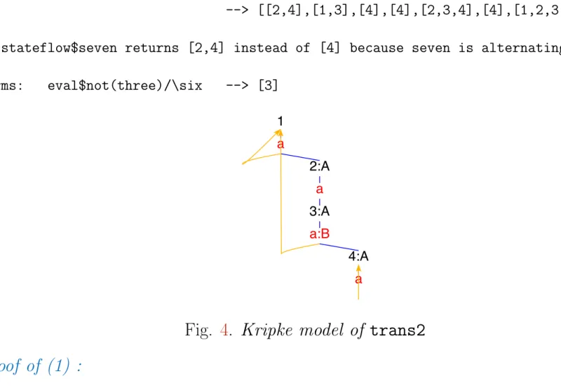
-- stateflow$seven returns [2,4] instead of [4] because seven is alternating terms: eval$not(three)/\six --> [3]
1 a
2:A a 3:A a:B
4:A a
Fig. 4. Kripke model of trans2 Proof of (1) :
0. Derivation of all(NOTTHREE)[1,3]
Equation removal is safe.
1. SIMPLIFYING the preceding trees (one step) leads to NOTTHREE(1) & NOTTHREE(3)
2. Adding
(NOTTHREE0(z0) <=== z0 = 1 | z0 = 3) to the axioms and applying COINDUCTION wrt
(NOTTHREE(st) ===> (a<>(not(Sat(A))/\NOTTHREE))$st) at positions [] of the preceding trees leads to
A `NOTin` [A] & NOTTHREE0(4) & NOTTHREE0(2) | A `NOTin` [] & NOTTHREE0(1) The reducts have been simplified.
3. NARROWING the preceding trees (one step) leads to NOTTHREE0(1)
The axioms have been MATCHED against their redices.
The reducts have been simplified.
4. NARROWING the preceding trees (one step) leads to True
The axioms have been MATCHED against their redices.
The reducts have been simplified.
Proof of (2):
0. Derivation of
THREE(st) & st `in` states ==> st = 2 | st = 4 All simplifications are admitted.
Equation removal is safe.
1. SHIFTING SUBFORMULAS at positions [0,1] of the preceding trees leads to THREE(st) ==> (st `in` states ==> st = 2 | st = 4)
2. Adding
(THREE0(st) ===> (st `in` states ==> st = 2 | st = 4))
to the axioms and applying FIXPOINT INDUCTION wrt (THREE(st) <=== (a#(Sat(A)\/THREE))$st)
at positions [] of the preceding trees leads to
(A `in` [A] & A `in` [] ==> False) & (THREE0(2) & A `in` [] ==> False) &
(A `in` [A] & THREE0(1) ==> False) & (THREE0(2) & THREE0(1) ==> False) &
(THREE0(4) & A `in` [] ==> False) & (THREE0(4) & THREE0(1) ==> False) The reducts have been simplified.
3. NARROWING the preceding trees (one step) leads to THREE0(1) ==> False
The axioms have been MATCHED against their redices.
The reducts have been simplified.
4. NARROWING the preceding trees (one step) leads to True
The axioms have been MATCHED against their redices.
The reducts have been simplified.
Graphical representations of the set of states satisfying (3)
◦ enter map(eval)[three,not$three,four,five,six,seven,eight] into the text field
press parse up; press simplify
◦ enter map(evalG)[three,not$three,four,five,six,seven,eight] into the text field press parse up; press simplify; enter drawS into the entry field
press tree > tree; press paint; adapt red support points and press combis to remove them
[]
1 a
2 a 3 a
4 a
1 a
2 a 3 a
4 a
1 a
2 a 3 a
4 a
1 a
2 a 3 a
4 a
1 a
2 a 3 a
4 a
1 a
2 a 3 a
4 a
1 a
2 a 3 a
4 a
For the simplification steps of
map(stateflow)[three, not$three, four, five, six, seven, eight]
and
stateflow$not(three)/\six,
see stateflow3.html and stateflow4.html, respectively.
Acceptors and regular expressions
-- reglangs
constructs: a b c d e h aa gg pp vv final q qa qb qab q1 q2
defuncts: delta beta plus unfold unfoldND unfoldBro reg draw drawC
preds: Unfold
fovars: e st st' w k m axioms:
states == [q] & labels == [a,b] & atoms == [final]
(q,a) -> qa & (q,b) -> qb &
(qa,a) -> q & (qa,b) -> qab &
(qb,a) -> qab & (qb,b) -> q &
(qab,a) -> qb & (qab,b) -> qa &
(q,a) -> q & (q,b) -> q1 &
(q1,a) -> q2 & (q1,b) -> q1 &
(q2,a) -> q1 & (q2,b) -> q1 &
final -> q & -- A1 acceptor of words with an even number of a's and an even -- number of b's if started in q
final -> qb & -- A2: acceptor of words with an even number of a's and an odd -- number of b's if started in q
final -> q1 & -- A3: acceptor of reg$11 (Unfold(st)[] <=== final -> st) &
(Unfold(st)(x:w) <=== (st,x) -> st' & Unfold(st')$w) &
unfoldND$w == out <=< kfold(flip$transL)$w & -- nondeterministic unfold -- (for kfold see base) delta(st,x) == head$transL(st)$x &
beta$st == ite(null$out$st,0,1) &
unfold(st) == beta.foldl(delta)(st) & -- deterministic unfold -- regular expressions
plus$e == e*star(e) &
reg$1 == star$plus(a)+plus(b*c) & --> star(a+b*c)
reg$2 == a+a*a*star(a)*b+a*b*star(b)+b & --> star(a)*b+a*star(b)
reg$3 == a+star(a)+eps+a & --> star(a)
reg$4 == (a+eps)*star(a)*(eps+a) & --> star(a) reg$5 == (a+eps)*star(a+eps)*(a+eps)+a+eps & --> star(a)
reg$6 == star(a)*b*star(b+eps)*(b+eps)+star(a)*b & --> star(a)*b*star(b) reg$7 == d*pp+c*h*e+a*b+c+a+a*b*c*d+star(a*a+b+a*b)+mt+c*aa+b*gg+eps+
a+a*a+vv+a*a*8+d+b &
--> (a*a*8)+a+(c*aa)+c+d+(a*b*c*d)+(c*h*e)+(b*gg)+(d*pp)+
-- star((a*a)+(a*b)+b)+vv reg$8 == a+((b+eps)*star(b+eps)*a)+
((a+((b+eps)*star(b+eps)*a))*star(a+b+eps+(mt*star(b+eps)*a))*
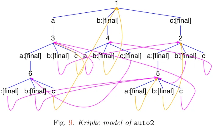
(a+b+eps+(mt*star(b+eps)*a))) & -- auto3 --> star(b)*a*star(a+b)
reg$9 == a+c+eps+((a+c+eps)*star(a+c+eps)*(a+c+eps))+
((b+((a+c+eps)*star(a+c+eps)*b))*star(a+b+eps+(c*star(a+c+eps)*b))*
(c+(c*star(a+c+eps)*(a+c+eps)))) & -- auto4
--> star(a+c)+(star(a+c)*b*star(a+b+(c*star(a+c)*b))*c*star(a+c)) -- autoToReg.minimize.regToAuto --> star(a+c+b*star(a+b)*c)
reg$10 == star(a)+star(a)*b*star(c*star(a)*b)*c*star(a) &
reg$11 == star(a)*b*star(a*(a+b)+b) &
-- widget interpreters
draw(m) == wtree(m)$fun((eps,k,n),text$eps, (st,k,n),ite(Int$st,
color(k,n)$circ$11, frame$blue$text$st)) &
drawC == wtree $ fun(eps,gif(cat,16,14),x,text$x) conjects:
Unfold(q)[] & --> False -- unify & narrow
Unfold(q)[b] & --> True -- derive & simplify & refute Unfold(q)[b,b] & --> False
Unfold(q)[a,b,a,b,a,b,a] & --> True -- reglangs1 Unfold(q)[a,b,a,b,b,a,b,a] & --> False
Unfold(q)[a,b,a,a,b,a] & --> False Unfold(q)[a,b,a,a,b,a,b] --> True terms:
unfoldND[q][] <+> --> [] -- simplify
unfoldND[q][b] <+> --> [final]
unfoldND[q][b,b] <+> --> []
unfoldND[q][a,b,a,b,a,b,a] <+> --> [final]
unfoldND[q][a,b,a,b,b,a,b,a] <+> --> []
unfoldND[q][a,b,a,a,b,a] <+> --> [] -- 39 steps unfoldND[q][a,b,a,a,b,a,b] <+> --> [final] -- 45 steps unfold(q)[a,b,a,a,b,a] <+> --> 0 -- 23 steps unfold(q)[a,b,a,a,b,a,b] <+> --> 1 -- 26 steps unfold(qgg)[a,b,a,a,b] <+> --> 0 -- 22 steps unfold(qgg)[a,b,a,a,b,a] <+> --> 1 -- 25 steps unfoldBro(reg$2)[a,a,a,b] <+> --> 1
unfoldBro(reg$2)[a,a,a,b,b] <+> --> 0
auto$reg$1 <+> --> non-deterministic acceptor of reg$1 pauto$reg$1 --> deterministic acceptor of reg$1
q:final
a b
qa qb
a b a b
qab a b
q
a b
qa qb:final
a b a b
qab a b
[0,4,3]
a b
[2,6,1] : final
a
[8]
a b
b
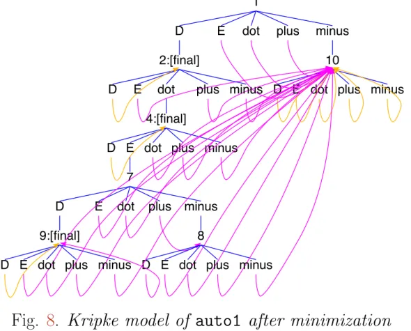
A1, A2 and the minimal acceptor of reg$11 that is isomorphic to A3 and whose state names were created by powerAuto (see below)
The following nondeterministic automaton (with initial state 0, final state 1 and -transitions) accepts the language of the regular expression reg1 = (a
++ (bc)
+)
∗. It results from sim- plifying auto$reg$1.
An application of drawL to the graph on the left leads to the graph on the right. The
rotation by 90 degrees is achieved by drawing the graph in painter mode t1-90.
0 eps 2 1 eps
4 6
a b
5 8
eps c
3 7
eps eps
eps b c a 0 2
1 2 4 6 3 2 1
4 5
5 4 3
6 8
7 6 3
8 7
The following equivalent deterministic automaton (with initial state [0,2,1,4,6] and final states [0,2,1,4,6], [5,4,3,2,1,6] and [7,6,3,2,1,4]) results from simplifying pauto$reg$1 or entering reg$1 into the solver text field and pressing specification > build Kripke model from regular expression.
[0,2,1,4,6]
a b
[5,4,3,2,1,6]
c [8]
a
[]
b c a b c a b c
[7,6,3,2,1,4]
a b c
[0,2,1,4,6]
a b c
[8] []
a b c a b c
Transitions of pauto$reg$1 - before and after minimization
Again, the minimal automaton was obtained by pressing specification > minimize after-
wards (see section 7).
Data type, parser and unparser for regular expressions
data RegExp = Mt | Eps | Const String | Sum_ RegExp RegExp | Prod RegExp RegExp | Star RegExp deriving Eq parseRE :: Sig -> TermS -> Maybe (RegExp,[String])
-- list of labels of acceptors parseRE _ (F "mt" []) = Just (Mt,[])
parseRE _ (F "eps" []) = Just (Eps,["eps"])
parseRE sig (F a []) = if sig.isDefunct a then Just (Var a,[a]) else Just (Const a,[a]) parseRE _ (F "+" []) = Just (Mt,[])
parseRE sig (F "+" [t]) = parseRE sig t
parseRE sig (F "+" ts) = do pairs <- mapM (parseRE sig) ts let (e:es,ass) = unzip pairs Just (foldl Sum_ e es,joinM ass) parseRE _ (F "*" []) = Just (Eps,["eps"])
parseRE sig (F "*" [t]) = parseRE sig t
parseRE sig (F "*" ts) = do pairs <- mapM (parseRE sig) ts let (e:es,ass) = unzip pairs Just (foldl Prod e es,joinM ass) parseRE sig (F "plus" [t]) = do (e,as) <- parseRE sig t
Just (Prod e $ Star e,as) parseRE sig (F "star" [t]) = do (e,as) <- parseRE sig t
Just (Star e,as `join1` "eps")
parseRE sig (F "refl" [t]) = do (e,as) <- parseRE sig t
Just (Sum_ e Eps,as `join1` "eps") parseRE _ (V x) = Just (Var x,[x])
parseRE _ _ = Nothing
showRE :: RegExp -> TermS
showRE Mt = leaf "mt"
showRE Eps = leaf "eps"
showRE (Const a) = leaf a
showRE e@(Sum_ _ _) = case summands e of [] -> leaf "mt"
[e] -> showRE e
es -> F "+" $ map showRE es showRE e@(Prod _ _) = case factors e of [] -> leaf "eps"
[e] -> showRE e
es -> F "*" $ map showRE es showRE (Star e) = F "star" [showRE e]
showRE (Var x) = V x
The following binary RegExp-relation are subrelations of regular language inclusion. In their defining equations, = means reverse implication.
instance Ord RegExp -- used by summands
where Eps <= Star _ = True
e <= Star e' | e <= e' = True
Prod e1 e2 <= Star e | e1 <= e && e2 <= Star e = True
Prod e1 e2 <= Star e | e1 <= Star e && e2 <= e = True e <= Prod e' (Star _) | e == e' = True
e <= Prod (Star _) e' | e == e' = True
Prod e1 e2 <= Prod e3 e4 = e1 <= e3 && e2 <= e4 e <= Sum_ e1 e2 = e <= e1 || e <= e2
e <= e' = e == e'
(<*) :: RegExp -> RegExp -> Bool -- used by factors Sum_ Eps e <* Star e' | e == e' = True
e <* e' = False
(<+) :: RegExp -> RegExp -> Bool -- Eps <+ e, e1*e2 <+ e3*e4 iff e1 <+ e3 Eps <+ e = True -- products are ordered by left factors Const a <+ Const b = a <= b
e@(Const _) <+ Prod e1 e2 = e <+ e1 e@(Star _) <+ Prod e1 e2 = e <+ e1 Prod e _ <+ e'@(Const _) = e <+ e' Prod e _ <+ e'@(Star _) = e <+ e' Prod e _ <+ Prod e' _ = e <+ e'
e <+ e' = e == e'
(+<) :: RegExp -> RegExp -> Bool -- Eps +< e, e1*e2 <+ e3*e4 iff e2 <+ e4 Eps +< e = True -- products are ordered by right factors Const a +< Const b = a <= b
e@(Const _) +< Prod e1 e2 = e +< e2
e@(Star _) +< Prod e1 e2 = e +< e2 Prod _ e +< e'@(Const _) = e +< e' Prod _ e +< e'@(Star _) = e +< e' Prod _ e +< Prod _ e' = e +< e'
e +< e' = e == e'
Flattening sums and products
summands,factors :: RegExp -> [RegExp]
summands (Sum_ e e') = joinMapR (<=) summands [e,e'] -- e <= e' ==> e+e' = e'
summands Mt = [] -- mt+e = e
summands e = [e] -- e+mt = e
factors (Prod e e') = joinMapR (<*) factors [e,e'] -- e <* e' ==> e*e' = e'
factors Eps = [] -- eps*e = e
factors e = [e] -- e*eps = e
joinMapR :: Ord b => (a -> [b]) -> [a] -> [b]
joinMapR f = foldl (foldl insertR) [] . map f insertR :: Ord a => [a] -> a -> [a]
insertR s@(x:s') y | y <= x = s
| x <= y = insertR s' y
| True = x:insertR s' y insertR _ x = [x]
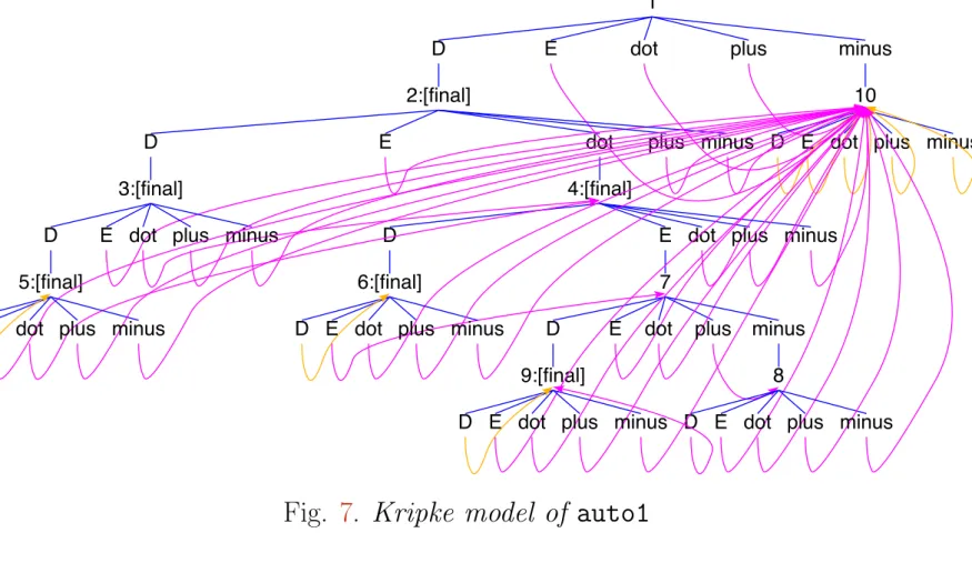
![Fig. 11. Kripke models from [4], Example 3.3.1.](https://thumb-eu.123doks.com/thumbv2/1library_info/4748942.1619786/162.977.253.775.56.704/fig-kripke-models-from-example.webp)

