The representation of location by a regional climate model in complex terrain

(1)

www.hydrol-earth-syst-sci.net/19/3449/2015/

doi:10.5194/hess-19-3449-2015

The representation of location by a regional climate model in complex terrain

D. Maraun¹and M. Widmann²

1GEOMAR Helmholtz Centre for Ocean Research Kiel, Düsternbrooker Weg 20, 24105 Kiel, Germany

2School of Geography, Earth and Environmental Sciences, University of Birmingham, Birmingham, B15 2TT, UK Correspondence to: D. Maraun (dmaraun@geomar.de)

Received: 10 February 2015 – Published in Hydrol. Earth Syst. Sci. Discuss.: 16 March 2015 Revised: 20 July 2015 – Accepted: 21 July 2015 – Published: 6 August 2015

Abstract. To assess potential impacts of climate change for a specific location, one typically employs climate model simulations at the grid box corresponding to the same geographical location. For most of Europe, this choice is well justified.

But, based on regional climate simulations, we show that simulated climate might be systematically displaced com- pared to observations. In particular in the rain shadow of mountain ranges, a local grid box is therefore often not representative of observed climate: the simulated windward weather does not flow far enough across the mountains; local grid boxes experience the wrong air masses and atmospheric circulation. In some cases, also the local climate change signal is deteriorated. Classical bias correction methods fail to correct these location errors. Often, however, a distant simulated time series is representative of the considered observed precipitation, such that a non-local bias correction is possible. These findings also clarify limitations of bias correcting global model errors, and of bias correction against station data.

1 Introduction

Many impacts of climate change are expected to manifest themselves at regional and local scales. To guide adaptation to these impacts, high-resolution climate scenarios are often desired that realistically simulate potential future regional climate. These scenarios are usually generated by dynamical or statistical downscaling of global climate model simulations (Rummukainen, 2010; Maraun et al., 2010). In the following we will only consider dynamical downscaling by regional climate models (RCMs), but later discuss our results

in a general context. For a regional climate change simulation to be useful, it should in general accurately represent the local marginal distribution (i.e. the unconditional prob- ability density function), present-day variability at daily to inter-annual scales, and the local response to climate change (Maraun et al., 2010); in specific cases, of course, further as- pects might be desired (Maraun et al., 2015).

Impact assessments for a specific location are typically based on simulations at the grid box corresponding to the same geographical location (or a combination of neighbouring grid boxes). This at first thought very reasonable choice is taken in several settings: when directly interpreting the local climate model output; also when driving an impact model representing a specific real-world area; and finally when bias correcting local model simulations against observed data.

In many cases, this choice will be justified and the best option. We argue, however, that it is not a priori clear whether a geographical model location represents the same real-world location. The orography even of high-resolution RCMs is in general a coarse model of the true orography.

As a consequence, in particular in mountain ranges, the simulated mesoscale flow might considerably deviate from the observed flow, resulting in systematically displaced local events. In the following we will demonstrate that in such cases, choosing local model output might result in a wrong simulation of climate variability and long-term trends, and thus in a wrong simulation of climate impacts. We refer to the representation of a real-world geographical location as location representativeness.

Testing the location representativeness is straightforward in weather forecasting by means of forecast verification: a high forecast skill indicates that the model indeed represents

(2)

Here we demonstrate the relevance of location representativeness for precipitation simulated by an RCM across Eu- rope, in particular in complex terrain. We propose to measure location representativeness by correlations between observations and simulations at the inter-annual scale. Often, in our setting, a very simple non-local bias correction can substantially improve location representativeness. Finally, we discuss consequences for correcting global climate model errors.

2 Concept and data

Location representativeness of RCM-simulated climate can in principle be measured by the temporal correlation between simulated and observed climate in a perfect boundary setting.

However, internal climate variability hampers the estimation.

An RCM, even if driven with perfect boundary conditions, is not designed to correctly simulate the observed day-to-day variability at the grid-box scale (Weisse and Feser, 2003;

Wong et al., 2014); away from the boundary conditions, complex weather dynamics will always result in consider- able random deviations of simulated from observed weather system trajectories. Although such mesoscale internal atmospheric variability reduces the correlation between simulation and observations, it does not reduce the location representativeness. Yet, mesoscale internal atmospheric variability generally occurs at short timescales and will be averaged out at longer timescales.

We therefore propose to measure location representativeness in a perfect boundary setting by the correlation between seasonally averaged observed and simulated time series. This timescale is a compromise between a high signal-to-noise ratio (boundary forced signal vs. random mesoscale weather variability) and a sufficient number of time steps. Thus, given an observed time series at seasonal scale,y_{ij k}in a grid box (i, j) fork =1 . . . Ntime steps, and a corresponding simulated time series x_{ij k}, we estimate the local location representativeness as

R_ij=C_k x_{ij k}, y_{ij k}

, (1)

R_ij^mn=C_k x_mnk, y_{ij k}

. (2)

A non-local representativeness measure can then be defined as

Re_ij=max_mnR_ij^mn; (3)

i.e. instead of representing local climate by the model grid box (i, j), one can chose that grid box that maximises the correlation between model and observation (m, n)=arg max_mnR_ij^mn. To reduce computational cost and to limit spurious correlations from very distant grid boxes, we consider non-local correlations in an 11×11 field centered on the observational grid box of interest.

To eliminate artificial non-local skill, all non-local mea- sures are calculated on a cross-validated series. The idea is to remove cases where a neighbouring grid box is chosen that just by chance has a higher correlation with local observations over the calibration period, but that would be less representative under prediction. To this end, the data have been divided into three blocks of 10- and one of 11-year length.

Each block is left out once and, for a chosen grid box in the observations, an individual non-local representative grid box (i.e. the location potentially varies from block to block) is determined by maximising the correlation across the 11×11 field in the remaining calibration blocks. The simulated data of that grid box for the left-out validation block are then writ- ten into the cross-validated series. Based on this series the final cross-validated non-local correlation is calculated. As marginal distributions might differ from grid box to grid box (and correlations are invariant to scale), all time series are transformed to zero mean and unit standard deviation prior to the cross-validation. As this cross-validation makes sense only for non-local representativeness, but not for the local measure, it can in some cases result in non-local representativeness values that are slightly lower than the corresponding – not cross-validated – local representativeness values.

To illustrate the concept, we consider precipitation simulated by the RCM RACMO2 from the KNMI (Konin- klijk Nederlands Meteorologisch Instituut, Royal Nether- lands Meteorological Institute) (van Meijgaard et al., 2008).

The RCM is forced by ERA40 reanalysis data at the lateral

(3)

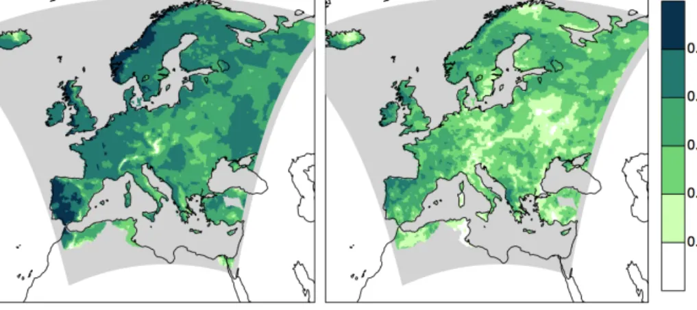
Figure 1. Local representativeness. Correlation between local (at the same grid box) simulated and observed seasonal mean time series. Left panel: DJF; right panel: JJA. Under the assumption of independence, correlationsC_k>0.3 are pointwise statistically significant at the 95 % level.

boundaries and operates at a 0.22^◦×0.22^◦horizontal resolution. The simulation spans the time period 1 January 1961–

31 December 2000 and is available from the ENSEMBLES project (van der Linden and Mitchell, 2009). As observational reference we employ the E-OBS data set (Haylock et al., 2008). Limitations of this data set have been high- lighted, in particular at the daily scale (Hofstra et al., 2010;

Kysely and Plavcova, 2010; Maraun et al., 2012), but the quality at the seasonal scale is generally high.

3 Results

Figure 1 shows local correlations between observed and simulated seasonal mean precipitation time series. For DJF (left panel) correlations over most of Europe are significant and high, in particular over western Europe and its elevated costal regions. The overall decrease in correlations from west to east reflects the growing influence of internal climate variability on the predominantly westerly flow away from the western boundaries. Thus, the gradient does not imply a decreasing representativeness towards eastern Europe, but sim- ply a decreasing signal-to-noise ratio. Along coastal regions with pronounced orography, precipitation is very well represented by RCMs (Eden et al., 2014): the track of a weather system is hardly diverted over the open ocean; orographic up- lift then triggers precipitation across a large area. The overall high correlations indicate that systematic errors in the large- scale circulation play a minor role for RCMs driven with perfect boundary conditions.

To discuss location representativeness, the white areas in mountainous regions are of interest, in particular the Alps, the Bohemian Massif and the eastern slopes of the Sierra Nevada in Spain. Here, the local model–observation correlation is insignificant, suggesting the presence of systematic orography-caused errors at the regional scale.

For summer (right panel), the correlations are lower across Europe; in large regions, insignificant. Patterns are patchy, and the orographic structure that is visible in winter mostly disappears. Insignificant correlations occur predominantly over eastern Europe and are readily explained by the continental climate: a large fraction of precipitation stems from local convective precipitation, which is controlled by local radiative heating rather than by large-scale atmospheric flow, making the resulting process almost independent of the boundary forcing even at the seasonal scale. During summer, the westerly flow is also much less pronounced (Greatbatch and Rong, 2006; Folland et al., 2009), furthermore decreasing the signal-to-noise ratio for identifying orography-caused errors. To summarise: during summer, internal climate variability limits the assessment of RCM location representativeness. Results for spring and autumn are in between those for winter and summer, with much less pronounced local effects but a systematic west–east gradient with less visible effects in more continental climates (see supplementary information).

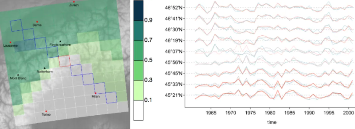
To investigate whether the vanishing correlations in mountainous areas are really caused by systematic local orographic effects, we estimate non-local correlations (Eq. 2). Figure 2, left panel, illustrates the approach for a grid box in the lee- ward foothills of the Alps (close to Domodossola in northern Italy). Each grid box shows the correlation between simulated precipitation in that grid box and observed precipitation in the central grid box against the real-world topography.

Correlations are high along the main ridge of the Alps and towards the north-west, but low in the Po Valley. In fact, observed precipitation in the central grid box is not represented by the corresponding RCM simulation, but rather by simulated precipitation on the windward side of the Alps. Other studies have found precipitation biases in the rain shadows of mountain ranges, often towards too little rain (e.g. Caldwell et al., 2009; Heikkilä et al., 2011); here we additionally show that not only the intensity is reduced because too much pre-

(4)

Figure 2. Location representativeness illustrated with a grid box in the Alps (around 46^◦07⁰N, 8^◦15⁰E) for winter (DJF). Left panel:

correlation of observed grid-box series with surrounding simulated series; red square: position of observational grid box; blue squares: cross section considered in (b); grey shading: real-world topography (Amante and Eakins, 2009). Right panel: seasonal mean time series along the cross section from (a). Blue: observed; red: model at the same grid box; grey: model at the grid box showing the highest correlation at inter-annual scale. The saturation of the red series indicates the correlation between model and observed series at the same grid box. Series are transformed to common mean and unit standard deviation.

cipitation occurs on the windward side of the mountains, but also that the whole weather (in terms of precipitation variability) does not cross the mountains. In other words: in reality, the Alpine foothills in the rain shadow of the main ridge are substantially influenced by the windward weather north- west of the Alps; in the RCM, the rain shadow is basically cut off from the north-western influence and resembles more the weather of the Po Valley. A closer look at the temporal variability in a cross section through the two mountain ranges confirms the above line of argument. The right panel of Fig. 2 shows observed and simulated precipitation time series for nine grid boxes from north-west to south-east, centered on the central grid box shown in the left panel. In the observations (blue lines), the transition from the windward side to the rain shadow of the Alps is rather smooth, whereas an abrupt change occurs in the RCM simulation (red lines) from the fourth to the fifth grid box (which is the location of the Bernese Alps with peaks ranging up to 4274 m; Finster- aarhorn)¹. For all nine grid boxes, at least one RCM simulated time series from a (potentially) distant grid box (grey lines) correlates well with the local observed precipitation time series.

The fact that in some regions non-local correlations are substantially higher than local correlations suggests representing local observed precipitation by precipitation simulated for a distant grid box according to Eq. (3). The cor-

1In principle, the change in correlation could be caused by prob- lems in the E-OBS data set rather than in the RCM. It is conceivable that at the given location, no observed stations were present, and all information in E-OBS is taken from the windward side of the Alps.

Given that the phenomenon occurs systematically along the whole main ridge of the Alps (and other ridges as well), such an artefact is very unlikely. For the region considered in Fig. 2, several stations south of the main Alpine ridge entered the E-OBS data set.

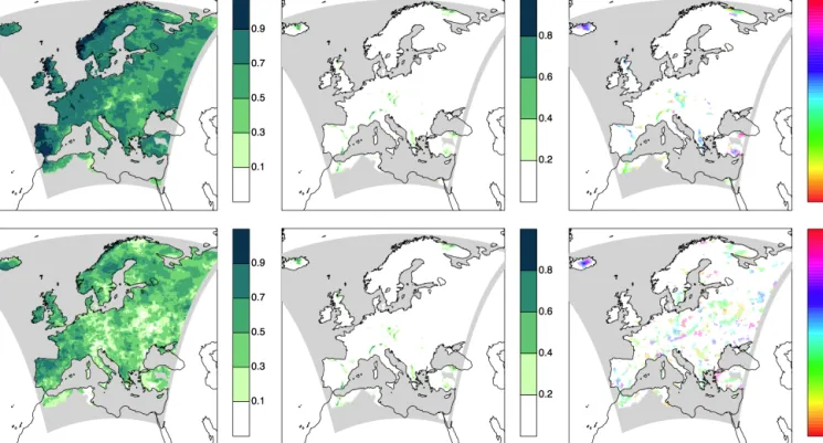
responding non-local correlation maps are shown in Fig. 3 for winter (top) and summer (bottom). For almost the en- tire Europe, at least one non-local grid box has been identi- fied that well represents local observed precipitation variability during winter. In particular in winter, the areas affected by orography errors with insignificant correlations have almost completely disappeared. For summer, the result is again dominated by internal weather variability. The middle panels show the improvement in correlations by the non-local approach: in particular over those mountainous areas, where the local RCM simulation did not well represent observed precipitation, correlations have greatly improved during winter.

The right panels indicate the direction of the non-local RCM grid box relative to the considered grid box that maximises the correlation between model and observations (only where the correlation improves by at least 0.2). During winter, the representative grid boxes lie in general towards the west or northwest of the considered grid box, demonstrating that the two examples really represent a general behaviour. Dur- ing summer, no clear directional pattern emerges, illustrat- ing again the influence of internal climate variability. Again, spring and summer show a large west–east gradient and re- semble winter in western Europe, but show much less systematic effects further to the east (Supplement).

The previous analysis has shown that, in particular in mountain areas, RCM-simulated precipitation at a specific location does not necessarily represent the observed precipitation variability on inter-annual scales. Therefore the ques- tion arises whether the climate change signal at such loca- tions might be wrongly represented by the RCM. We thus compare the linear trends (in percent per decade) in observed seasonal precipitation with the local simulated trend as well as the simulated trend for the grid box with highest location representativeness. Note that we are not interested in separat-

(5)

Figure 3. Non-local representativeness. Top panels: DJF; bottom panels: JJA. Left panels: correlation between observed seasonal mean time series and modelled time series at a non-local grid box that maximises correlation with observations; centre panels: improvement in correlation by using non-local series; right panels: direction of a model grid box that maximises correlation relative to the local grid box.

Areas where correlation does not improve by at least 0.2 are shown in white.

Figure 4. Reduction in absolute trend bias by the non-local approach. Trends measured in percent per decade. Left panel: DJF; right panel:

JJA. Green: improvement (bias reduced); brown: deterioration (bias increased). Areas where correlation does not improve by at least 0.2 are shown in grey. As the cross-validation would cause inhomogeneities, trends are calculated without cross-validation.

ing externally forced trends, but just in overall linear trends as they manifest in both observed and simulated time series.

As both are synchronised on inter-annual timescales, their trends are also comparable.

Figure 4 depicts the improvement in simulated trends com- pared to observed trends (reduction in absolute trend bias) when considering non-local representativeness. We show only results for grid boxes where the non-local approach im-

proves correlations by at least 0.2. Green indicates an improvement, brown a deterioration. During winter (left), almost no grid boxes show a deterioration in the representation of trends by the non-local approach; many grid boxes indicate no change. A large fraction, however, shows an improvement in the simulated trends when considering non- local representativeness. For summer (right), the picture is again erratic, with about as many improvements as deteriora-

(6)

aggregated precipitation separately for winter and summer.

For most of Europe, location representativeness is high;

the chosen RCM well represents the corresponding local climate. But, in particular in the rain shadow of major mountain ranges such as the Alps, RCM precipitation might not be representative of the actually observed precipitation at a chosen grid box. Earlier studies (e.g. Caldwell et al., 2009;

Heikkilä et al., 2011) have shown that precipitation is often biased towards too low values in the rain shadows of mountain ranges. Here we demonstrate that not only the marginal distributions are biased, but also that the simulated climate is not representative of the observed climate. In fact, the simulated windward weather does not cross the mountain range to the extent it does in reality. Thus, the local grid box ex- periences the wrong air masses and the wrong atmospheric circulation, which both make up inter-annual variability. In some cases, also the local climate change signal is deteriorated. These results could be clearly demonstrated for winter. In summer, the assessment of location representativeness is complicated because mesoscale internal climate variability dominates boundary forcings even on inter-annual scales.

Our findings have some immediate implications for bias correction. Classical local bias correction methods – in the sense of mapping a local simulated surface variable onto the observed one at the corresponding geographical location (Déqué et al., 2007; Maraun et al., 2010; Teutschbein and Seibert, 2012) – will fail to correct these location errors. Such bias correction methods adjust marginal distributions: they are an ad hoc post processing of e.g. the magnitude of temperature values or precipitation intensities, but they do not shift air masses or change the atmospheric circulation. We therefore argue that for mountain regions it is essential to test for location representativeness prior to any bias correction.

If a distant simulated time series is found to be representative of the considered observed precipitation, a non-local bias correction is in general possible. As a first simple approach, one could adapt the idea of Widmann et al. (2003) and map the best representative distant simulated time series onto local observations. Such a correction would not only adjust marginal distributions, but additionally “shift the weather across the mountains”: the corrected simulation would experience the right air masses and atmospheric circulation.

ting, situations are conceivable where no grid box correctly represents the point location. If the local weather is mainly determined by local orographic phenomena (e.g. a mountain breeze, valley fog), the simulated grid box average (in fact, even gridded observational data) might only contain little relevant information about the local climate (Maraun, 2014). In such a situation a meaningful bias correction would be im- possible. Thus, also here it is crucial to test for location representativeness, in particular in complex terrain.

Often, it is desired to correct the combined RCM and global climate model errors, or even to directly bias correct global climate models against observations. In such a setting it is difficult to test location representativeness as simulations and observations are not temporally aligned. Here, a location correction conditional on weather types (which have to be jointly defined in observations and the global model) might provide a way forward. In fact, as such a correction would directly include information about the relevant physical causes of the biases – the displacement should mainly depend on the mesoscale flow – it should in principle be very robust in terms of stationarity of location biases under climate change.

Additionally to mesoscale errors induced by orography, global climate models typically suffer from large-scale circulation errors such as a displacement of the storm tracks (e.g.

Randall et al., 2007). In other words: in general, simulated climate at a particular geographical location is not representative of the corresponding local observed climate. Thus, in line with the argument of Eden et al. (2012) and Eden and Widmann (2014), at a given location it is not a priori clear whether a bias correction of global climate models is justified. Prior to any bias correction one should therefore assess whether the relevant dynamical processes governing a local climate of interest are well simulated and well located.

The preceding discussion broadens the concept of representativeness. In addition to the location aspect discussed here, representativeness has a well-known scale aspect: climate models simulate area average values and thus do not represent point data of station observations (Klein Tank et al., 2009). Also here, the root of the problem is not the difference in marginal distributions, but the fact that area averages do not contain all information about local-scale variations (Ma- raun, 2013). Again, a classical deterministic bias correction

(7)

would fail; a stochastic bias correction, however, could in principle add the required small-scale variability (Maraun, 2013; Wong et al., 2014).

The Supplement related to this article is available online at doi:10.5194/hess-19-3449-2015-supplement.

Acknowledgements. We thank E. Meredith for helpful discussions and acknowledge financial support by the Volkswagen Foundation, Az. 85 423. M. Widmann has been supported by a short-term scientific mission of EU COST Action ES1102 VALUE. RCM data are available from hhtp://ensemblesrt3.dmi.dk, E-OBS data from http://www.ecad.eu.

The article processing charges for this open-access publication were covered by a research

centre of the Helmholtz Association.

Edited by: L. Samaniego

References

Amante, C. and Eakins, B.: ETOPO1 1 Arc-Minute Global Re- lief Model: Procedures, Data Sources and Analysis, NOAA Technical Memorandum NESDIS NGDC-24, NOAA (National Oceanographic and Atmospheric Administration), Boulder, Col- orado, USA, 19 pp., 2009.

Caldwell, P., Chin, H.-N., Bader, D., and Bala, G.: Evaluation of a WRF dynamical downscaling simulation over California, Cli- matic Change, 95, 499–521, 2009.

Déqué, M., Rowell, D. P., Luthi, D., Giorgi, F., Christensen, J. H., Rockel, B., Jacob, D., Kjellström, E., de Castro, M., and van den Hurk, B.: An intercomparison of regional climate simulations for Europe: assessing uncertainties in model projections, Climatic Change, 81, 53–70, 2007.

Eden, J. and Widmann, M.: Downscaling of GCM-simulated precipitation using Model Output Statistics, J. Climate, 27, 312–

324, 2014.

Eden, J., Widmann, M., Grawe, D., and Rast, S.: Skill, Correction, and Downscaling of GCM-Simulated Precipitation, J. Climate, 25, 3970–3984, 2012.

Eden, J., Widmann, M., Maraun, D., and Vrac, M.: Comparison of GCM- and RCM-simulated precipitation following stochastic postprocessing, J. Geophys. Res., 119, 11040–11053, 2014.

Folland, C., Knight, J., Linderholm, H., Fereday, D., Ineson, S., and Hurrell, J.: The Summer North Atlantic Oscillation: Past, Present, and Future, J. Climate, 22, 1082–1103, 2009.

Glahn, H. R. and Lowry, D. A.: The use of Model Output Statistics (MOS) in objective weather forecasing, J. Appl. Meteorol., 11, 1203–1211, 1972.

Greatbatch, R. J. and Rong, P.-F.: Discrepancies between Differ- ent Northern Hemisphere Summer Atmospheric Data Products, J. Climate, 19, 1261–1273, 2006.

Haylock, M. R., Hofstra, N., Klein Tank, A. M. G., Klok, E. J., Jones, P. D., and New, M.: A European daily high- resolution gridded data set of surface temperature and precipitation for 1950–2006, J. Geophys. Res., 113, 20119, doi:10.1029/2008JD010201, 2008.

Heikkilä, U., Sandvik, A., and Sorteberg, A.: Dynamical downscaling of ERA-40 in complex terrain using the WRF regional climate model, Clim. Dynam., 37, 1551–1564, 2011.

Hofstra, N., New, M., and McSweeney, C.: The influence of in- terpolation and station network density on the distributions and trends of climate variables in daily gridded data, Clim. Dynam., 35, 841–858, 2010.

Klein Tank, A., Zwiers, F., and Zhang, X.: Guidelines on Analysis of extremes in a changing climate in support of informed deci- sions for adaptation, Climate data and monitoring wcdmp-no. 72, World Meteorological Organisation, Geneva, Switzerland, 2009.

Kysely, J. and Plavcova, E.: A critical remark on the applicabil- ity of E-OBS European gridded temperature data set for validat- ing control climate simulations, J. Geophys. Res., 115, D23118, doi:10.1029/2010JD014123, 2010.

Maraun, D.: Bias Correction, Quantile Mapping and Downscaling:

Revisiting the Inflation Issue, J. Climate, 26, 2137–2143, 2013.

Maraun, D.: Reply to Comment on “Bias Correction, Quantile Map- ping and Downscaling: Revisiting the Inflation Issue”, J. Cli- mate, 27, 1821–1825, 2014.

Maraun, D., Wetterhall, F., Ireson, A. M., Chandler, R. E., Kendon, E. J., Widmann, M., Brienen, S., Rust, H. W., Sauter, T., The- meßl, M., Venema, V. K. C., Chun, K. P., Goodess, C. M., Jones, R. G., Onof, C., Vrac, M., and Thiele-Eich, I.: Precipita- tion downscaling under climate change, Recent developments to bridge the gap between dynamical models and the end user, Rev.

Geophys., 48, RG3003, doi:10.1029/2009RG000314, 2010.

Maraun, D., Osborn, T. J., and Rust, H.: The influence of synptic air- flow on UK daily precipitation extremes, Part II: regional climate model and E-OBS data validation, Clim. Dynam., 39, 287–301, 2012.

Maraun, D., Widmann, M., Gutierrez, J. M., Kotlarski, S., Chan- dler, R. E., Hertig, E., Wibig, J., Huth, R., and Wilcke, R. A. I.:

VALUE: A Framework to Validate Downscaling Approaches for Climate Change Studies, Earth’s Future, 3, 1–14, 2015.

Randall, D. A., Wood, R. A., Bony, S., Colman, R., Fichefet, T., Fyfe, J., Kattsov, V., Pittman, A., Shukla, J., Srinivasan, J., Stouf- fer, R. J., Sumi, A., and Taylor, K. E.: Climate Change 2007:

The Physical Science Basis, Contribution of Working Group I to the Fourth Assessment Report of the Intergovernmental Panel on Climate Change, in: chap. Climate Models and Their Evaluation, Cambridge University Press, Cambridge, UK and New York, NY, USA, 2007.

Rummukainen, M.: State-fo-the-art with regional climate models, Wiley Int. Rev. Clim. Change, 1, 82–96, doi:10.1002/wcc.8, 2010.

Teutschbein, C. and Seibert, J.: Bias correction of regional climate model simulations for hydrological climate-change impact studies: Review and evaluation of different methods, J. Hydrol., 456, 12–29, 2012.

van der Linden, P. and Mitchell, J. F. B.: ENSEMBLES: Climate Change and its Impacts: Summary of research and results from the ENSEMBLES project, Tech. rep., Met Office Hadley Centre, Exeter, UK, 2009.

(8)