Aspects of noncommutativity and holography in field theory and string theory

(1)

Aspects of Noncommutativity and Holography in Field Theory and String Theory

D I S S E R T A T I O N

zur Erlangung des akademischen Grades doctor rerum naturalium

(dr. rer. nat.) im Fach Physik eingereicht an der

Mathematisch-Naturwissenschaftlichen Fakult¨ at I Humboldt-Universit¨ at zu Berlin

von

Herr Dipl.-Phys. Christoph Sieg geboren am 09.10.1974 in Hagen

Pr¨ asident der Humboldt-Universit¨ at zu Berlin:

Prof. Dr. J¨ urgen Mlynek

Dekan der Mathematisch-Naturwissenschaftlichen Fakult¨ at I:

Prof. Thomas Buckhout, PhD Gutachter:

1. Dr. Harald Dorn 2. Prof. Dr. Dieter L¨ ust 3. Dr. Jan Plefka

eingereicht am: 14. Mai 2004

Tag der m¨ undlichen Pr¨ ufung: 12. August 2004

(2)

(3)

iii

To my parents

(4)

(5)

v

Abstract

This thesis addresses two topics: noncommutative Yang-Mills theories and the AdS/CFT correspondence.

In the ﬁrst part we study a partial summation of the θ-expanded perturbation theory.

The latter allows one to define noncommutative Yang-Mills theories with arbitrary gauge groups G as a perturbation expansion in the noncommutativity parameter θ. We show that for G ⊂ U(N), G = U(M), M < N, one does not find a finite set of θ-summed Feynman rules.

In the second part we study quantities which are important for the realization of the holographic principle in the AdS/CFT correspondence: boundaries, geodesics and the propagators of scalar ﬁelds. They should play a role in the holographic setup in the BMN limit as well. We observe how these quantities behave in the limiting process from AdS₅×S⁵ to the 10-dimensional plane wave which is the spacetime in the BMN limit.

Keywords:

Noncommutative Yang-Mills theory Feynman rules

AdS/CFT and BMN correspondence Holographic principle

(6)

Zusammenfassung

Die Arbeit besch¨aftigt sich mit zwei Themen: den nichtkommutativen Yang-Mills- Theorien und der AdS/CFT-Korrespondenz.

Im ersten Teil wird eine teilweise Aufsummation der θ-entwickelten St¨orungstheorie untersucht. Letztere stellt einen Weg dar, nichtkommutative Yang-Mills-Theorien mit beliebigen Eichgruppen Gals Störungsentwicklung im Nichtkommutativitätsparameter θ zu definieren. Es wird gezeigt, daß man im Fall G⊂ U(N), G =U(M), M < N keinen endlichen Satz von θ-summierten Feynman-Regeln finden kann.

Im zweiten Teil werden Bausteine untersucht, die für eine Realisierung des holo- graphischen Prinzips in der AdS/CFT-Korrespondenz von Bedeutung sind: Ränder, Geodäten und die Propagatoren skalarer Felder. Sie sollten auch für eine holographische Formulierung im BMN Limes wichtig sein. Das Verhalten dieser Größen im Limesprozeß von AdS₅ ×S⁵ zu der 10-dimensionalen ebenen Gravitationswelle, welche die Raumzeit im BMN-Limes ist, wird studiert.

Schlagw¨orter:

Nichtkommutative Yang-Mills-Theorie Feynman-Regeln

AdS/CFT- und BMN-Korrespondenz Holgraphisches Prinzip

(7)

Part I

Introduction

(12)

(13)

Chapter 1 General Introduction

In the energy range accessible with present experiments, three of the four fundamental interactions are successfully described by quantum ﬁeld theories. The latter provide a theoretical description of the strong, weak and electromagnetic interactions which are col- lectively denoted as the Standard Model (of particle physics). The remaining interaction is gravity and its classical description is given by the theory of General Relativity.

The quantum field theories in the Standard Model are all examples of gauge theories, where spin one particles are responsible for transmitting the interaction. Gauge theories contain more degrees of freedom than necessary for the description of the physical (measurable) quantities. The gauge transformations relate physically equivalent field configurations, and thus form a group such that a sequential application of two gauge transformations is itself a gauge transformation. For example, the gauge group of the Standard Model is given by SU(3)×SU(2)×U(1), where the first factor refers to the theory of the strong interaction which is called quantum chromodynamics (QCD), and the second and third factors describe the electroweak interaction that includes the weak and the electromagnetic parts. In addition to the gauge fields, a gauge theory may contain additional fields the gauge fields interact with. In the case of the Standard Model these are the fermionic quark and lepton fields and the scalar Higgs field.

Naively, one would expect that a direct observation of the particles that are associ- ated with the Standard Model ﬁelds is possible in their elementary form. Depending on the interaction, one furthermore should ﬁnd several compound systems of the elementary particles, bound together by the fundamental forces. But this naive expectation is not quite true. For instance, one does not observe free quarks. The hadrons, which are bound

(14)

states of the the strong interaction, behave differently compared to electromagnetic bound states. Consider for instance positronium which is a state of an electron and a positron bound via the electromagnetic force. If one separates the electron from the positron, the force of electromagnetism decreases, and it is possible to break up a positronium into its elementary constituents. In contrast to this, trying to separate two quarks inside the hadron leads to an effectively constant force, corresponding to an effective potential which is linearly increasing with the distance. Hence at a certain point, where the potential energy is high enough to create a quark anti-quark pair, the hadron breaks up into two hadrons, such that one does not find free quarks. A necessary (but not sufficient) ingredient for this behaviour is the interaction of the gauge bosons with each other. This is one of the main differences between QCD and quantum electrodynamics (QED) and is due to the gauge group of QCD being non-Abelian, whereas QED has an Abelian gauge group.

The absence of unbound quarks in nature makes it diﬃcult to show their existence.

Hence, it becomes understandable that before the formulation of QCD, much work was spent in trying to explain the spectrum of hadrons without taking into account that they might be non-fundamental composite objects. One of the surprising issues of the hadronic spectrum is that the hadrons can be sorted into groups in such a way that, within every group, one finds a linear relation between the mass squares m² of the hadrons and their spins J. In the linear relation αm² = α0 +J the slope α ∼ 1 GeV⁻² is universal for all hadrons, only the intercept α₀ is different for each group of hadrons. If one plots m² versus J one obtains the famous Regge trajectories [146, 147]. They were realized within dual models¹ [159, 181, 183] which successfully describe the behaviour of hadron scattering amplitudes in the so called Regge regime. For example, a 2 → 2 scattering process in four dimensions is specified by the three Mandelstam variables s, t and u as kinematical invariants. Only two of them, choose for instance s and t being related to the center of mass energy and the scattering angle in the process, are independent. In the Regge regime, which is given by s → ∞ with t = fixed, the scaling behaviour of the scattering amplitude proportional to s^α(t) with α(t) =α₀+αt is successfully reproduced by the dual models. It was discovered [126, 128, 167] that the dual models describe the dynamics of relativistic strings and thus we will henceforth denote them as (hadronic) string theories.

1For an introduction with a detailed summary of the historical developments see [154].

(15)

5

Besides the above outlined successes these string theories contain some issues that are unwanted in a theory of hadrons. They predict the existence of a variety of massless particles not detected in the hadronic spectrum. Depending on the concrete model, different values for the intercept α0 are theoretically favoured² that are in disagreement with the phenomenologically preferred valueα₀ = ¹₂. Furthermore, the behaviour of the scattering amplitudes in the hard fixed angle scattering regime, where s and t are large with fixed ratio ^s_t, is too soft compared to the experimental results. Here the string theories predict an exponential falloff, while experimentally one finds a powerlike behaviour. Experimen- tal data indicate that the probed structure in this regime is not an extended object but instead a pointlike particle. This means that the probe particles no longer interact with the hadron as a whole but with pointlike constituents from which the latter is built.

Hence, a theory of hadrons is not a theory of fundamental objects. It turned out that QCD is the appropriate description of the constituents from which hadrons are built. But the strong interactions are far from being understood completely. Perturbative QCD is very successful in describing the phenomenology of strong interactions at high energies but the effects at low energy, where the coupling constant is large and hence perturbation theory is not applicable, are still hard to analyze. The absence of free quarks described above is an effect of this property called confinement, that until now cannot be successfully explained. The hadronic string theories can be interpreted as effective descriptions of confinement where the open string collects the effects of the flux tubes transmitting the forces between the quarks that are situated at the endpoints of this QCD string (see e. g. [39, 141, 143, 144, 157] and references therein). To be able to analyze quantum field theories non-perturbatively and thereby understand the mechanism of confinement beyond such an effective description is a challenge for theoretical physics.

Besides this fact there is another lack of understanding. General Relativity is the relevant theory of gravity at length scales that are large compared to the fundamental length of gravity, the Planck lengthlP=M_P⁻¹ (MP = 1.22×10¹⁹GeV is the Planck mass).

But a description of gravity at very short distances comparable to the Planck length requires a quantum theory of gravity. The naive attempt to quantize general relativity fails. To be more precise, quantum ﬁeld theories suﬀer from divergencies that have to be regularized and absorbed into the physical parameters of the theory. This procedure is known as renormalization. In contrast to QCD and the electroweak interaction which

2An enhancement of symmetries [184] and the decoupling of negative norm states [38,80] is found.

(16)

are renormalizable quantum ﬁeld theories³, naive quantum gravity is non-renormalizable.

The fields with highest spin for which a quantum field theoretical description is known are the spin one gauge fields, but the graviton (the quantum of gravitation) carries spin two.

One fundamental diﬀerence between gravity and gauge theories is that spacetime itself is aﬀected by gravity and hence is dynamical. A good way to understand this is to think about what happens if one wants to observe smaller and smaller structures in spacetime.

The probe wavelength has to be comparable or smaller than the minimum length one wants to resolve. This means one has to put higher and higher energy into the system.

Energy is a source of gravitation and hence the spacetime is deformed in the measurement process. This is a good reason why the spacetime at small scales of the order of magnitude of the Planck length would look diﬀerently from what one observes at large scales. In particular, if one increases the energy above a critical value, the gravitational collapse of the region would be inevitable and the desired information would be absorbed by the black hole which would form. The density of quantum states of a black hole turns out to depend on the area of the horizon and it suggests that only one bit of information can be stored in a surface element of the order of the squared Planck length [168, 175, 176]. Hence, a formulation of quantum gravity should include a mechanism that makes it impossible to resolve structures that are smaller than the Planck length. This clearly introduces an upper bound on momenta and hence an ultraviolet cutoﬀ in the quantum theory.

One way to realize such a cutoﬀ is to introduce extended objects to replace the pointlike particles as fundamental objects. Heuristically speaking, to smear out interactions and make them non-local prohibits one from probing the spacetime at arbitrarily small scales.

The string theories, that originally appeared as a proposal to describe the hadrons, are theories of 1-dimensional extended objects. If they are formulated as a theory of gravity [155] where nowα ∼M_P⁻², the disadvantage that occurred in the form of the exponential falloﬀ of the amplitudes then turns into an advantage to guarantee a nice high energy behaviour. Moreover, the appearance of the unwanted massless modes is important.

These modes contain the desired graviton. Quantization leads to constraints on the dimension and the shape of the spacetime in which the string theories live. The so called critical dimension which is necessary for a consistent quantum theory of strings is much higher than four, in particular it is given by D= 26 and D = 10 for the bosonic and the

3See [172,173,177] and further references given in [47,124].

(17)

1.1 Noncommutative Yang-Mills theories 7

supersymmetric string theories, respectively.⁴ The additional dimensions do not rule out string theories as theories of gravity. Since we do not know how spacetime looks like at short distances comparable to the Planck length, there is the possibility that additional compact dimensions exist. They should simply be highly curved and thus so tiny that it is impossible to detect them at energy scales that are accessible today. Much better, the additional dimensions naturally lead to a uniﬁed description of gauge theories and gravity in our four-dimensional perspective.

Besides fixing the dimension, the consistency of the quantum theory further restricts the choice of a classical background on which the string theories can be formulated. By classical background we mean that one specifies a spacetime plus values for the fields of the theory. A consistent classical background has to fulfill certain differential equations that at the leading order turn out to be the Einstein equations for the metric and the Yang-Mills field equations for gauge fields. This means that at energies small compared to the Planck scale one finds string theories encompass general relativity [155, 188, 189]

and gauge theories [127].

Putting together all the above given observations, string theories are promising can- didates for a uniﬁed formulation of the four fundamental interactions [155]. In the following will not review string theories further and refer the reader to the literature [82,83,110,139, 140].

The next two Sections contain a short introduction and motivation of the two topics we are dealing with in this thesis. A short summary of the structure of the corresponding part will be given at the end of each of these sections.

1.1 Noncommutative Yang-Mills theories

We have seen that the understanding of quantum field theories and of quantum gravity is highly relevant for a successful description of all fundamental interactions. Quantum field theories and in particular Yang-Mills (YM) theories are far from being understood completely. One way to learn more about them is to analyze modified YM theories which

4It is not strictly necessary to work in the critical dimension. The price to pay is that the worldsheet metric becomes dynamical even in conformal gauge and introduces one new degree of freedom. Another possibility is to work with a non-constant dilaton such that the critical dimension is modiﬁed. This clearly breaks Poincar´e invariance in the target space.

(18)

do not necessarily play a direct role in the description of nature.

For instance, one can deform the spacetime on which YM theories are formulated.

The case of a noncommutative spacetime is of particular interest. In the canonical case that will be of importance here, the commutator of two spacetime coordinates x^µ and x^ν is given by

[x^µ,x^ν] =iθ^µν , (1.1)

whereθ^µν is a constant tensor that necessarily has length dimension two. In this way one has introduced a new parameter

θ into the theory that can be used as an expansion parameter for a perturbative analysis.⁵

Noncommutativity gives rise to a topological classification of Feynman diagrams [23, 174]. One replaces each line of a graph by a double line such that one obtains the so called ribbon graphs. The genus h of a Feynman diagram is then defined as the minimal genus of all surfaces on which its ribbon graph can be drawn without the crossing of lines. It then turns out that planar diagrams in the noncommutative theory are given by essentially the same expressions that one finds in the ordinary (commutative) theory.

The only diﬀerence is that an overall phase factor multiplies each planar graph, being the same for each graph with ﬁxed external momenta [72].

The situation is diﬀerent for non-planar diagrams. Inside the loop integrals of the corresponding expressions, phase factors occur in the noncommutative case that depend on the loop momentumk. In the limit of larger and largerθ^µν these phase factors oscillate with smaller and smaller period and hence they increasingly suppress the non-planar contributions. Particularly, in the perturbation expansion for maximal noncommutativity, i. e.θ^µν → ∞ or alternatively all momenta being large at ﬁxedθ^µν, only planar diagrams survive. Hence, ¹_θ plays the role of a topological expansion parameter, i. e. θ is the analog of the rank N of the gauge group in the large N genus expansion [174] that will be described in Section1.2 below.

Making spacetime coordinates noncommutative is not only useful for learning more about gauge theories. In addition it enables one to study some aspects of gravity without using gravity itself. The noncommutativity of the coordinates gives rise to the non-locality of interactions. Hence, one can study the inﬂuence of non-locality on renormalization properties in the framework of gauge theories and one avoids to work with theories of

5θ denotes the maximum of the absolute values of all entries ofθ^µν in its canonical skew-diagonal form, see [171].

(19)

1.1 Noncommutative Yang-Mills theories 9

gravity. Noncommutativity and hence non-locality of the interactions do not improve the ultraviolet behaviour of planar diagrams since only a multiplicative phase factor arises.

Non-planar diagrams, however, behave differently. The oscillatoric behaviour of the phase factors inside the loop integrals renders all one-loop non-planar diagrams finite⁶. This gives rise to the remarkable issue of UV/IR mixing [121]. The effective UV cutoff depends on the external momenta p in such a way that the UV divergencies reappear whenever pµθ^µν →0. This means that at small momenta the noncommutative phase factors inside the loop integrals are irrelevant and hence turning on noncommutativity replaces the standard ultraviolet divergencies with a singular infrared behaviour.

As we have seen before, non-locality and improved high energy behaviour of the amplitudes should be important ingredients in a theory of quantum gravity. The facts that noncommutative YM theories capture some aspects of gravity and that gravity naturally occurs in string theories, leads to the question of how deeply gauge and string theories are related. Could it be possible that some gauge and string theories describe the same physics? Before describing examples of this kind in section 1.2, we motivate and summarize the analysis in Part II of this thesis.

During investigating noncommutative ﬁeld theories one could have the idea of simpli- fying the problem by studying a truncated version of the full noncommutative theory. One expands in powers ofθ^µν and only considers some of the leading terms. However, in such an expansion eﬀects like UV/IR mixing are lost. They require the full θ^µν-dependence.

On the other hand, a frequently addressed task in the context of noncommutative gauge theories is their consistent formulation for gauge groups different fromU(N). In contrast to the case of ordinary gauge theories this question is highly non-trivial since a priori noncommutative theories appear to be consistent only for U(N) gauge groups. In some approaches that deal with such a modification, an explicit expansion in powers of θ^µν is required and this prevents one from studying effects like UV/IR mixing for these theories.

Part II deals with the question of how compatible the extension of noncommutative YM theories to arbitrary gauge groups is with keeping the exact dependence on the noncommutativity parameter θ^µν.

• In Chapter 2 we start with a review of how noncommutative YM theories arise from string theories. This connection implies the existence of a map between the

6This does not hold for all non-planar diagrams at higher loops.

(20)

noncommutative and the ordinary description. The map is of particular importance in a formulation of noncommutative YM theories with arbitrary gauge groups.

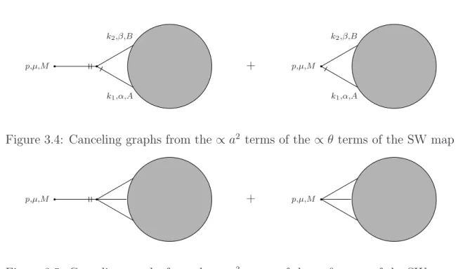
• In Chapter 3 we introduce noncommutative YM theories. We review the effects of noncommutativity on the choice of the gauge group. Then we present the Faddeev- Popov gauge fixing procedure and use it to derive the map between the noncommutative and ordinary ghost fields. We will first extract the well-known Feynman rules for noncommutative U(N) YM theories. We summarize the aforementioned approaches of how to implement other gauge groups in noncommutative gauge theories. Based on our work [61], we will then discuss what happens in a construction of θ^µν exact Feynman rules if the gauge group is a subgroup ofU(N).

• A short introduction to the used formalism as well as some detailed calculations that are useful for ﬁxing notations and support the analysis of PartII are collected in Appendix A.

1.2 Dualities of gauge and string theories

In 1974 ’tHooft [174] found a property of SU(N) gauge theories that suggests a relation to string theory. He observed that the perturbation expansion can be regarded as an expansion in powers of λ = g²N instead of an expansion in powers of the YM coupling constantg. In addition to the expansion inλ, one can classify Feynman graphs in powers of N⁻². A perturbative expansion in N⁻² is possible in the case of large N with λ kept fixed. It can be interpreted with the help of the double line notation for Feynman graphs [23, 174], that was already introduced in section 1.1. Here, each line now represents one fundamental index of theN×N representation matrices of the gauge group. The largeN expansion then turns out to be a topological expansion in which a Feynman diagram with genushis of orderN⁻^2h. If one now takes the so called ’tHooft limit, whereN → ∞andλ is kept fixed, only the planar graphs which can be drawn on a sphere (h = 0) survive. The genus expansion of Feynman diagrams in a gauge theory resembles the genus expansion of string theory, such that a relation between these two different types of theories was conjectured.

(21)

1.2 Dualities of gauge and string theories 11

1.2.1 The AdS/CFT correspondence

The ﬁrst concrete example of a gauge/string duality was proposed by Maldacena in 1997 [113] and is known as AdS/CFT correspondence in the literature. One case of particular importance is the conjecture that the 4-dimensional supersymmetric (N = 4) YM theory should describe the same physics as type II B string theory on an AdS₅×S⁵ background with some additional Ramond-Ramond ﬂux switched on.

Up to now the conjecture could not be analyzed in full generality, but it has passed several non-trivial checks. One regime in which concrete computations can be done on the string theory side is where the string theory can be replaced by type II B supergravity. On the gauge theory side this regime corresponds to ﬁrst taking N → ∞at ﬁxed λand then takingλ→ ∞. It is therefore perfectly inaccessible with perturbation theory. But turning the argument around, if one assumes that the AdS/CFT correspondence is correct, then there is a nice tool to analyze this concrete gauge theory in the large N limit at strong

’tHooft coupling λ by working in the dual supergravity description.

How can it happen that a lower dimensional gauge theory contains the same amount of information as the higher dimensional string theory? The physical picture behind this is that the AdS/CFT correspondence is holographic. Since this issue is one of the main motivations for Part III of this thesis, let us explain it in more detail.

Originally if we were to talk about holography we refer to a particular technique in photography. The use of a coherent light source like a laser enables one to store not only brightness and colour information of a three dimensional object on the two dimensional film. One splits the laser beam into two parts such that one hits the film directly and the other hits the object on the side that is directed towards the film. The direct part of the beam and the light that is reflected from the object generate an interference pattern that is stored on the film. The result is that one has encoded information about the varying distance between the surface of the object and the film. Viewing a holographic film, the object then appears three dimensional and the part that was directed towards the film could in principle be completely reproduced without information loss, at least if the resolution of the film were arbitrarily high. This is in sharp contrast to the ordinary photography which is simply a (orthogonal) projection, such that all the information about length scales perpendicular to the film is lost. In the real case of a finite resolution of the film there is an information loss in both cases, both images appear blurred at

(22)

suﬃciently small distances. But the essential diﬀerence between the holographic and the ordinary image, that one does or does not have any information about the third dimension, remains.

In quantum gravity, holography [168, 175, 176] appears in connection with a black hole which information is stored on its horizon. The holographic screen is the horizon and a single grain of the ﬁlm corresponds to an area element of Planck size. It is the minimum area on which information can be stored. One could now argue [176] that the emergence of holography in this context is only a special case of a holographic principle that is of universal validity in theories of gravity. Indeed, the holographic principle plays an essential role in connection with the AdS/CFT correspondence.

Let us now draw the analogy to the AdS/CFT correspondence. The complete three dimensional space in the photography example becomes the 5-dimensional anti-de Sitter spacetime AdS₅.⁷ The lower dimensional holographic screen which corresponds to the two dimensional film in the above example is given by the 4-dimensional boundary of AdS₅. The easiest way to understand this is to represent AdS₅ as a full cylinder. The boundary of the cylinder then is the holographic screen and the radial coordinate is the coordinate perpendicular to the film. It is called the holographic direction. Strings live in the full cylinder, and the four dimensional theory lives on its boundary. The interference pattern that encodes the position perpendicular to the screen in holographic photography corresponds to the energy scale in the boundary theory. Like in the case of the black hole, the Planck length corresponds to the finite resolution of the film [168].

Although one finds many similarities between holographic photography and the AdS/CFT correspondence one should not drive the analogy too far. In contrast to photography where it should in principle not matter where the screen is put, in the AdS/CFT correspondence this choice can have non-trivial effects. The reason is that the geometry is not only given by AdS₅ but instead by the 10-dimensional product space AdS₅×S⁵. For instance, the choice to take the boundary of AdS₅ as a holographic screen implies that it is four dimensional, because there the S⁵ is shrunk to a point. Any slice at a constant holographic coordinate value somewhere in the interior of AdS5 ×S⁵ is 9-dimensional because there the S⁵ has finite size. Hence, such a slice would define a 9-dimensional holographic screen. Indeed, this difference is one main reason why in a certain limit of

7The additional 5-dimensional sphere to form a 10-dimensional spacetime simply produces the Kaluza- Klein tower of states.

(23)

the AdS/CFT correspondence a unique holographic description has not yet been found.

Before we describe this limit it is worth to recapitulate what happened with string theories until now. They were originally introduced to describe the strong interactions.

Then they were replaced by QCD that has many advantages but is little under control beyond perturbation theory. String theories were proposed as the theories of gravity. But they reentered the regime of gauge theories as possible dual descriptions that might be a key tool to study non-perturbative eﬀects in gauge theories.

This seems to explain why in their original formulation as theories of hadrons string theories covered some aspects of hadron physics. In particular it becomes more plausible why strings are an effective description of the QCD flux tubes. Furthermore, it sheds new light on the unwanted issues of string theories in this direct formulation describing hadrons. They could be regarded as a hint that one was working in the wrong setup (one should work in the spirit of the AdS/CFT correspondence instead of trying to formulate them directly as theories of hadrons) including the wrong choice of scales (one should use α ∼ M_P⁻² instead of α ∼ 1 GeV⁻²). For instance, it was indeed found that the too soft behaviour of string amplitudes in the hard fixed angle regime can be avoided in the framework of the AdS/CFT correspondence [142].

1.2.2 The BMN limit of the AdS/CFT correspondence

At the present time, a proof of the AdS/CFT correspondence is still out of reach. Even an analysis of string theory on AdS₅ ×S⁵ beyond the supergravity approximation lies outside present capabilities. Berenstein, Maldacena and Nastase [21] formulated a new limit of the AdS/CFT correspondence that goes beyond the supergravity approximation.

The proposal is based on the observation [28] that the AdS₅ ×S⁵ background can be transformed with the so called Penrose-Güven limit [88,135] to a plane wave background [27] on which string theory is quantizable [118,119]. Berenstein, Maldacena and Nastase translated the limit to the gauge theory side and proposed that a certain subsector of operators in the gauge theory should then be related to type II B string theory on the plane wave. This limit reveals further aspects of the presumably deep connection between gauge and string theories. A very nice picture is that the operators which are compound objects made from the fields of the gauge theory can be interpreted as discretized strings where each field operator represents a single string bit.

(24)

Later it was found [75,86] that the BMN limit can be embedded into the more general framework of expanding the string theory about a classical string solution on AdS₅×S⁵and that explicit checks for several classical solutions can be performed because the relevant gauge theory parts are integrable.

But what is still missing is a satisfactory description of how holography in the AdS/CFT correspondence appears in its BMN limit. Connected with this, it is not clear what the dual gauge theory is and where it lives. Is it a one dimensional theory on the one dimensional boundary of the plane wave spacetime, or does it live on a screen in the interior that could have any dimension between one and nine?

In Part IIIof this thesis we discuss the behaviour of some geometrical and ﬁeld theoretical quantities in the limiting process from the AdS/CFT correspondence to its BMN limit. The idea is that one should observe how quantities that are relevant in the holographic description are transformed in the limit and hence learn more about the fate of holography.

• In Chapter4we review the ingredients that are essential for an understanding of the backgrounds in the AdS/CFT correspondence and in its BMN limit. Furthermore, we will review the limiting processes with which some of the backgrounds can be related and which play an important role in understanding the idea of the AdS/CFT correspondence and how its BMN limit arises.

• In Chapter 5 we review how holography is understood in the AdS/CFT correspondence in more detail. We then turn our attention to its plane wave limit and give a brief summary of some work to deﬁne a holographic setup in the BMN limit. This gives an impression that the picture is less unique than in the AdS/CFT correspondence itself.

• In Chapter6we analyze how the boundary structure behaves in the limiting process.

Furthermore, to get some information on the causal structure, we derive and classify all geodesics in the original background and discuss their fate in the limit. This Chapter is completely based on our analysis in [62].

• In Chapter 7 we come back to the arguments given in Chapter 5, that the propagators are ingredients of particular importance in a holographic setup. We focus on the bulk-to-bulk propagator in generic AdS_d+1 ×S^d⁺¹ backgrounds. We compute

(25)

it in particular cases and analyze some of its properties in detail. In particular, we show how the well-known result in the 10-dimensional plane wave spacetime is obtained by taking the Penrose limit. This chapter is mainly based on our analysis in [60].

• Some detailed calculations and useful formulas that refer to Part III are collected in Appendix B.

(26)

(27)

Part II

Noncommutative geometry

(28)

(29)

Chapter 2 Noncommutative geometry from string theory

The intention of this Chapter is to review how noncommutative gauge theories arise from open strings in the presence of a constant B-ﬁeld. There exist several approaches [1, 7–

9,43,45,46,63,156] to this problem but we will mainly follow the argumentation of [158].¹ First we will discuss the σ-model description and then later on we will focus on the low energy eﬀective action. Besides giving insights into the mechanism of how ﬁeld theories can be derived from string theories, the discussion leads us to an essential ingredient for our own analysis: the Seiberg-Witten (SW) map, which provides a translation between ordinary and noncommutative gauge theory quantities.

2.1 The low energy limit of string theory with con- stant background B -ﬁeld

2.1.1 σ-model description

The action of a bosonic string which propagates in a background consisting of a spacetime metric g_{M N}, an antisymmetric ﬁeld B_{M N} and a dilaton φ can be written as

S = 1 4πα

Σ

d²σ

δ^abg_{M N}(X)−2πiα^abB_{M N}(X)

∂_aX^M∂_bX^N +αRφ(X)

. (2.1) Here the string sweeps out a worldsheet Σ with scalar curvature R and we have chosen conformal gauge and work with Euclidean signature such that the worldsheet metric isδ_ab.

1See also the introduction in [179].

(30)

Furthermore, we assume a (D = 26)-dimensional target space which leads to a critical string theory where the worldsheet metric remains non dynamical in conformal gauge after quantization.² If the theory describes open strings we may add additional terms such as

−i

∂Σ

dt AM(X)∂X^M + 1 2π

∂Σ

dt k φ(X) (2.2)

to the action (2.1), which couple a background gauge ﬁeld A_M and the dilaton φ to the boundary ∂Σ of the worldsheet Σ. Here ∂ denotes the tangential derivative along the worldsheet boundary and k is the geodesic curvature of the boundary. If the 2-form B fulﬁlls dB = 0, which includes the case of a constantB_{M N}, and if the dilatonφis constant, the action for open strings can be cast into the form

S = 1 4πα

Σ

d²σ g_{M N}∂_aX^M∂^aX^N − i 2

∂Σ

dt

B_{M N}X^M + 2A_N

∂X^N +φχ , (2.3) where χ denotes the Euler number of the worldsheet Σ. The second integral shows that one can alternatively describe the constant B-field by a gauge field A_M = −¹₂B_{M N}X^N. The field strength derived from it is F_{M N} =B_{M N} with the usual definition

F_{M N} =∂_MA_N −∂_NA_M . (2.4)

Up to now the endpoints of the open strings can move unconstrained in the spacetime, the string obeys Neumann boundary conditions. In the framework of Dp-branes this setup corresponds to the case of a spacetime ﬁlling D(D−1)-brane. If instead we impose Neumann boundary conditions inp+ 1 dimensions and Dirichlet boundary conditions in the remainingD−p−1 dimensions, this deﬁnes the string endpoints to lie on a Dp-brane.

This means that they can move freely in p+ 1 spacetime directions and are stuck at ﬁxed positions in the remaining D−p−1 spatial dimensions. We split the coordinate indices in the following way

M, N = 0, . . . , D , µ, ν = 0, . . . , p , m, n=p+ 1, . . . , D , (2.5) such that capital Latin indices M, N, . . . run over all spacetime directions whereas lower case Greek (µ, ν, . . .) and Latin (m, n, . . .) indices denote directions respectively parallel and perpendicular to the Dp-brane. The boundary of the string worldsheet lies completely on the brane. This means that the coordinatesX^m|∂Σ are constant and thus∂X^m|∂Σ = 0.

2We of course choose string backgrounds which preserve the conformal invariance.

(31)

2.1 The low energy limit of string theory with constant background B-ﬁeld 21

Then only the componentsB_µν andA_ν along the brane contribute to the boundary term of (2.3) and we can set all other components to zero without loss of generality. To simplify the analysis we will now in addition assume that the ﬁeld B_µν on the Dp-brane has maximum rank and that the metric gM N is independent ofX^M and of block-diagonal form with respect to the coordinate split (2.5). The background ﬁelds then read

g_{M N} = g_µν 0 0 g_mn

, B_{M N} = B_µν 0

0 0

. (2.6)

In this setup the boundary terms in (2.3) (with A_N = 0) modify the boundary conditions of the open strings. One ﬁnds

X^m

∂Σ = 0 , g_µν∂_⊥+ 2πiαB_µν∂

X^ν

∂Σ = 0 (2.7)

for the directions perpendicular and parallel to the Dp-brane respectively. ∂_⊥ denotes the derivative normal to the boundary of the worldsheet. It is important to mention that the equations of motion are not aﬀected by the addition of the boundary terms in (2.3).

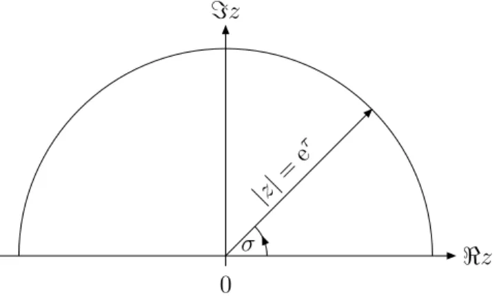
To analyze the theory with the boundary conditions (2.7) it is advantageous to choose coordinates (τ, σ) in which the boundary of the open string worldsheet is parameterized by τ and is located at constant σ = 0, π. The string worldsheet then describes a strip in the complex plane of w =σ−iτ which can be conformally mapped to the upper half plane via the holomorphic transformation z = e^iw = e^τ+iσ. The origin of the half plane corresponds to τ → −∞ and half circles around the origin refer to constant τ, see Fig.

2.1.

In these coordinates the boundary of the worldsheet is the real axis where z = ¯z and the derivatives ∂_τ and ∂_σ are given by

∂_τ =z∂ + ¯z∂ ,¯ ∂_σ =iz∂−i¯z∂ ,¯ ∂ = ∂

∂z , ∂¯= ∂

∂z¯ . (2.8) Using (2.6), the boundary conditions (2.7) then read in (z,z) coordinates¯

X^m

z=¯z = 0,

g_µν(∂−∂) + 2πα¯ B_µν(∂+ ¯∂)

X^µ

z=¯z = 0. (2.9)

Since the boundary terms in the action (2.3) do not modify the equations of motion, the propagator is standard for the directions perpendicular to the Dp-brane. The complete

(32)

z 0

z

|z|=e^τ σ

Figure 2.1: Description of the string worldsheet with the complex coordinate z. The worldsheet of the open string is given by the upper half plane with z ≥ 0 and its boundary is the real axis. A slice of constant worldsheet ‘time’ τ is given by a half circle with radius |z| = e^τ. The inﬁnite past and future are given by the origin and the circle with inﬁnite radius respectively.

solution with the boundary conditions (2.9) in the constant background (2.6) is given by [1,158]

X^µ(z)X^ν(z)

=−α

g^µνln|z−z|

|z−z¯| +G^µνln|z−z¯|²+ 1

2παθ^µνlnz−z¯

¯

z−z +D^µν

, X^µ(z)Xⁿ(z)

= 0, X^m(z)Xⁿ(z)

=−αg^mnln|z−z| ,

(2.10) where D^µν is a constant and we have used the abbreviations

GM N =gM N−(2πα)² B1

gB

M N , G^{M N} =

1 g+ 2παB

M N S

=

1

g+ 2παBg 1 g−2παB

M N

, θ^{M N} = 2πα

1 g+ 2παB

M N A

=−(2πα)²

1

g+ 2παBB 1 g−2παB

M N

.

(2.11)

They are related via

G^{M N}+ θ^{M N} 2πα =

1 g+ 2παB

M N

, (2.12)

which is trivially fulﬁlled for the directions (M, N) = {(m, ν),(µ, n),(m, n)}, where B_{M N} = 0, θ^{M N} = 0.

(33)

Due to the third term in the ﬁrst line of (2.10), the propagator is single-valued if the branch cut of the logarithm lies in the lower half plane. As a consistency check for (M, N) = (µ, ν) one recovers the propagator on the disk with Neumann boundary conditions [139] for Bµν = 0.

The quantities given in (2.10) and (2.11) have a simple interpretation. In conformal ﬁeld theories there exists a map between asymptotic states of incoming and outgoing ﬁelds and operators which are called vertex operators. If one wants to compute string theoretical scattering amplitudes one has to insert the vertex operators into the two dimensional surface. The topology of the latter determines the order in the string coupling constant and the type of vertex operators that can couple. Closed string vertex operators couple to all surfaces, inserting them at points in the interior. However, open string vertex require that the surface possesses a boundary where they have to be inserted.

The short distance singularity of two vertex operators that approach each other can either be read off from the propagator or from their operator product expansion. The anomalous dimensions of the vertex operators determine the short distance behaviour in the operator product expansion. Hence, one concludes that the singularity of the propagator (2.10) if two interior points coincide determines the anomalous dimensions of closed string vertex operators. From (2.10) one finds in this case that for (M, N) = (µ, ν) the only singular term is the numerator of the first logarithmic term which is similar to the term for (M, N) = (m, n). The short-distance behaviour is

X^M(z)X^N(z)

∼ −αg^{M N}ln|z−z| (2.13) and its coeﬃcient enters the expressions for the anomalous dimensions of the closed string vertex operators. Thus, g_{M N} is the metric seen by closed strings.

On the other hand since open strings couple to the disk by inserting the corresponding vertex operators into the boundary of the disk, their anomalous dimensions are determined by the short distance singularity of (2.10) for both points at the boundary, where z =

¯

z =s. One ﬁnds

X^µ(s)X^ν(s)

=−αG^µνln(s−s)²+ i

2θ^µν(s−s) , (2.14) with an appropriately chosen D^µν =−_2αⁱθ^µν and with

(s) =

−1 s <0

1 s >0 . (2.15)

(34)

Open string vertex operators see the metric G_µν. We will therefore denote G_µν as the open string metric.

We want to show that the sign function(s) in (2.14) is responsible for the non vanish- ing of the commutator of the two fieldsX^µ,X^ν at the same boundary point. Remember first that according to the previous discussion around fig.2.1, the radial coordinate of the half plane refers to the worldsheet ‘time’. ‘Time’ ordering therefore translates to radial ordering on the complex z plane. The equal time commutator of two fields is defined as the difference of two limits of the time ordered product of these fields. The first [second]

limit is to let the time coordinate of the second ﬁeld approach the time coordinate of the ﬁrst one from below [above]. The translation to radial ordering (denoted by R) is obvious and one obtains using (2.14)

X^µ(s), X^ν(s)

=

limε→0R

X^µ(s)X^ν(s−ε)−X^µ(s)X^ν(s+ε)

= i 2

θ^µν−θ^νµ

=iθ^µν . (2.16) The parameterθ^µνcan be interpreted as the noncommutativity parameter in a space where the embedding coordinates on the Dp-brane describe the noncommutative coordinates.

We will now determine the effect of the additional terms in (2.3) on string scattering amplitudes. As we have mentioned above, an element of the string S-matrix is a correlator of vertex operators that describe the asymptotic states. The correlators (at fixed order in the string coupling) are defined as a path integral over all fields X^M and metrics of the 2-dimensional surface of particular topology with vertex operators inserted and with the action (2.3) (with A_N = 0). An appropriate gauge fixing procedure is also understood.

Consider ﬁrst the simplest vertex operator for an open string tachyon with momentum p which is given by : e^ip^µ^X^µ:. Here : denotes normal ordering and indices are raised and lowered with the metric in (2.11). Using (2.14), the operator product of two open string tachyon vertex operators for s > s is given by

: eîp^·^X(s):: eîq^·^X(s):∼(s−s)^2α^p^·^qe⁻²ⁱ^θ^µν^p^µ^q^ν: eî(p+q)^·^X(s): , (2.17) where ‘∼’ denotes that we have only kept the most singular terms and we have defined p·q = G^µνp_µq_ν. One can capture the complete θ-dependence on the R. H. S. with the Moyal-Weyl ∗-product [122] which is defined as

f(x)∗g(x) = e²ⁱ^θ^µν^∂ξµ^∂ ^∂ην^∂ f(x+ξ)g(x+η)

ξ=η=0

(2.18)

(35)

and which is a special example of a noncommutative ∗-product, see Appendix (A.4) for some details. One especially ﬁnds for this product

x^µ∗x^ν−x^ν ∗x^µ=iθ^µν (2.19) in accord with (2.16). The product of two tachyon vertex operators (2.17) can then be written as

: e^ip^·^X(s):∗: e^iq^·^X(s):

X^µ(s)X^ν(s)_θ=0 = : e^ip^·^X(s):: e^iq^·^X(s):. (2.20) The above result means that the normal ordering of two tachyon vertex operators can either be performed by using (2.14) for contractions or alternatively by replacing the ordinary product with the ∗-product and contracting with the two point function (2.14) without the θ-dependent term. Both procedures capture the entire θ-dependence.

This discussion can be generalized to products of arbitrary open string vertex operators. A generic open string vertex operator is given by a polynomial P that depends on derivatives of the X and an exponential function to ensure the right behaviour under translations

V(p, s) = :P[∂X, ∂²X, . . .] eîp^·^X(s):. (2.21) If one now normal orders products of these vertex operators, one finds that only the exponential factors generate a dependence on θ^µν in contrast to the contractions which include at least one field of the polynomial prefactors. The reason for this is that in the two point function (2.14) theθ-dependent term can be disregarded if derivatives are taken and an appropriate regularization is used (like point splitting regularization in Subsection 2.1.3). Therefore, one obtains the sameθ-dependent exponential factor as if one had used tachyon vertex operators. It is now simple to see the θ-dependence of string amplitudes.

One has to insert the vertex operators into the boundary of the string worldsheet, and one has to integrate over the insertion points.³ In case of an n-point amplitude with vertex operators V_k,k = 1, . . . , none obtains

ⁿ

k=1

V_k(p_k, s_k)

G,θ

= exp −i

2

k>l

θ^µν(p_k)_µ(p_l)_ν(s_k−s_l) ⁿ

k=1

V_k(p_k, s_k)

G,θ=0

. (2.22) The subscript of a correlator denotes which parameters the correlator has to be computed with. The complete θ-dependence is thus described by the exponential prefactor if the

3Note that the gauge fixing procedure does not fix the worldsheet metric completely. Depending on the topology of the worldsheet, a remnant, the conformal Killing group (CKG), has to be fixed by inserting some vertex operators at fixed points without performing an integration. For the disk, three vertex operator positions have to be fixed.

(36)

theory is formulated in terms of the open string metric G_{M N}. Due to momentum con- servation the prefactor is invariant under cyclic permutations of the p_k. Performing the integrations of the above expression over (some of) the insertion points s_k then produces contributions with diﬀerent phase factors if the vertex operators exchange their positions in a non cyclic way. The appearance of the prefactor can be exactly described by the

∗-product (2.18) of the corresponding n ﬁelds, and one then rewrites (2.22) as

V₁(p₁, s₁)· · ·V_n(p_n, s_n)

G,θ =

V₁(p₁, s₁)∗ · · · ∗V_n(p_n, s_n)

G,θ=0 . (2.23)

The above expression is an important result for the discussion of the low energy eﬀective theory.

2.1.2 The Seiberg-Witten limit

In order to find the low energy description of the theory with action (2.3) one has to get rid of stringy effects in the correlation functions (2.23). It is clear that in an appropriate limit one should send to zero the parameter α, which is proportional to the square of the string length. In this case, where one wants to keep the effects of a constant B-field, one cannot simply keep constant the other parameters. As can be seen from (2.11), the B-dependence and especially θ^µν vanishes and one finds the same theory without initial B-field, if one keeps constant the other parameters in the limit. One should instead keep the open sting metric G_µν and θ^µν finite and different from zero. This is natural because the correlators (2.23) which will be discussed in the limit depend on these quantities and on α. In the Seiberg-Witten limit some components of the closed string metric g_µν and α are sent to zero at constant B-field in the following way

α ∼√

→0 , g_µν ∼→0 , g_mn = const., B_µν = const. (2.24) This then ensures that G_{M N} and θ^{M N} have reasonable limits. The expressions (2.11) become