Conformal Aspects of String Theory

(1)

DISS. ETH Nr. 17914

Conformal Aspects of String Theory

A B H A N D L U N G zur Erlangung des Titels

DOKTOR DER WISSENSCHAFTEN der

ETH Z ¨URICH

vorgelegt von

CHRISTOPH ANDREAS KELLER Dipl. Phys. ETH, ETH Z¨urich

geboren am 30. April 1981 von Bannwil BE

Angenommen auf Antrag von Prof. Matthias R. Gaberdiel, Referent

Prof. Ilka Brunner, Korreferentin

Prof. Bertram Batlogg, Studienvorsteher D-PHYS

2008

(2)

(3)

Abstract

This thesis deals with aspects of conformal field theory in string theory. It investigates two areas of string theory where two dimensional conformal field theory plays an important role: First, the dynamics of strings and branes are described by their worldsheet CFT and its boundary conditions. Second, the holographic dual of a string theory living on 2+1 dimensional anti-de Sitter space is also given by a two dimensional CFT.

The first part of this thesis investigates perturbations of the worldsheet CFT and the resulting renormalisation group flows: If a bulk theory is perturbed by inserting integrated marginal fields, a flow on the boundary may be induced which changes the brane configuration in such a way that the resulting theory is again conformal. Also, depending on the type of perturbation and the boundary condition, symmetries of the theory may or may not be broken. Conversely, the branes themselves may backreact on the bulk theory via contributions of higher order in the string coupling gs. These effects are analysed and the corresponding RG equations are obtained.

In a second part, the role of dual CFTs in the framework of the AdS/CFT correspondence is investigated. First, a proposal is made for the dual CFT of a specific configuration of heterotic strings, NS5 branes and Kaluza-Klein monopoles. Second, the existence of extremal CFTs is investigated. Extremal theories are proposed as holographic duals to pure quantum gravity in 2+1 dimensions. Checking this proposal in the bosonic case, one can use the formalism of Zhu to derive differential equations to test the consistency of a given theory. In the N = 2 supersymmetric case, the mere existence of the elliptic genus is already a non-trivial consistency test. Such methods are used to make statements on the existence of extremal CFTs.

(4)

(5)

Zusammenfassung

Die vorliegende Dissertation behandelt Aspekte von konformen Feldtheorien in der String- theorie. Es werden zwei Bereiche der Stringtheorie untersucht, in denen zweidimensionale konforme Feldtheorien eine wichtige Rolle spielen: Einerseits wird die Dynamik von Strings und Branes durch ihre Weltflächen-CFT und die zugehörigen Randbedingungen beschrieben. Andererseits ist die duale Randtheorie zu Stringtheorien, die auf 2+1 di- mensionalem anti-de Sitter-Räumen leben, ebenfalls wieder eine zweidimensionale CFT.

In einem ersten Teil werden Störungen der Weltflächen-CFT und die dabei entstehen- den Renormierungsgruppen-Flüsse untersucht: Wenn die Theorie mittels eingesetzter, integrierter marginaler Felder gestört wird, kann ein Fluss auf dem Rand der Theorie auftreten, der die Konfiguration der Branes dahingehend verändert, dass die resultierende Theorie wieder konform ist. Zudem können abhängig von der Art der Störung und der Randbedingung Symmetrien der ursprünglichen Theorie gebrochen werden. Andererseits können die Branes auch eine Rückwirkung auf die Bulk-Theorie bewirken durch Beiträge von Diagrammen höherer Ordnung in der String-Kopplungskonstante gs.

Im zweiten Teil wird die Rolle von dualen konformen Theorien im Rahmen der AdS/CFT- Korrespondenz untersucht. Es wird ein Vorschlag präsentiert für die duale CFT einer bestimmten Konfiguration von heterotischen Strings, NS5-Branen und Kaluza-Klein-Mo- nopolen. Anschliessend wird die Existenz von extremalen CFTs untersucht. Solche The- orien werden aufgestellt als holographische Dualtheorien zu reinen Quantengravitations- theorien in 2+1 Dimensionen. Im bosonischen Fall kann man den Zhu’schen Formalismus benutzen, um Differentialgleichungen herzuleiten, die die Konsistenz einer gegebenen The- orie überprüfen. Wenn die Theorie hingegen N = 2-Supersymmetrie aufweist, ist schon die Existenz des elliptischen Genus ein nicht-trivialer Konsistenztest.

(6)

(7)

Introduction

String theory

In nature, the interaction of all particles are governed by just four forces: gravity, elec- tromagnetism, the weak nuclear force, and the strong nuclear force. The laws of gravity are given by Einstein’s theory of general relativity, a classical field theory. The other three forces are described by quantum field theories (QFT). They are all explained by the standard model of high energy physics. The standard model is one of the most successful scientific theories of our time. It makes predictions on the interaction of particles which have been tested to an extremely high level of precision.

Nevertheless, we know that the standard model does not describe nature completely.

In particular, it does not incorporate gravity. There have been many attempts to find a theory which includes both the standard model and gravity, and so unifies all four forces.

Most candidate theories that have been found suffer from so-callednon-renormalisability: when calculating physical quantities, they give infinite expressions. For non-renormalisable theories, these infinities cannot be removed by the usual prescriptions. It thus remains an open problem to find a unified theory.

The most promising candidate for such a fully unified theory is string theory — see e.g. [114, 165] for an introduction and overview of the subject. String theory contains gravity in a very natural way. It also circumvents the problem of non-renormalisability by abandoning the idea of pointlike particles. Instead, one-dimensional objects are introduced: strings. There are two kinds of strings, closed strings and open strings. The endpoints of open strings can be fixed to a geometric surface, a D-brane. If one follows a string through time, it carves out a two-dimensional area of spacetime, the worldsheet.

The dynamics of a string is described by the two dimensional field theory that lives on its worldsheet. This worldsheet theory will be the main focus of the first part of this thesis.

Conformal field theory

The field theory on the worldsheet not only has the usual Poincar´e symmetries, but in addition also possesses conformal symmetry. Such theories are called conformal field theories (CFTs). They are invariant under rescaling, or, more precisely, under any map that preserves angles. This means that such theories do not contain any intrinsic length scale and no massive particles.

The size of the symmetry group depends greatly on the number of dimensions. For d >2 the number of symmetry generators is ¹₂(d+1)(d+2). Apart from the usual rotations

(12)

R and translations T, they also contain dilatations D and so-called special conformal transformations S. It is for d = 2 that the full power of the conformal symmetry group appears. Writing the worldsheet as the complex plane C with coordinate z, all analytic mapsz 7→f(z) are conformal. If we write down the Laurent series off(z) we see that that the symmetry group has an infinite number of generators. This gives an infinite number of constraints on the correlation functions. Some of these theories are thus exactly solvable by symmetry considerations alone. For an introduction to two dimensional CFTs, see e.g. [105, 48].

The second advantage of the two dimensional case is that it is possible to divide the theory into two sectors which are essentially independent of each other: the right-moving sector and left-moving sector, or alternatively, holomorphic and anti-holomorphic sector.

Invariance under dilatation requires that the energy-momentum tensor T be traceless.

Moreover, we can separate it into its holomorphic part T(z) and its anti-holomorphic part ¯T(¯z). We can then expand T(z) in terms of its modes,

T(z) = X

n∈Z

L_nz⁻ⁿ⁻^h . The Virasoro generatorsL_n satisfy the Virasoro algebra,

[Lm, Ln] = (m−n)Lm+n+ c

12m(m²−1)δm+n .

These commutation relations encode the conformal symmetry of the theory. In particular, all states decompose into represenation of the Virasoro algebra.

The second term on the right-hand side of the commutation relation, thecentral term, can be viewed as a quantum effect. The central charge c is a very important quantity when one tries to construct the worldsheet CFT of a string theory. It can be shown [114]

that bosonic string theory requiresc= 26, whereas the superstring requires c= 15. In a free theory, each boson gives a contribution ofc= 1, whereas a fermion contributesc= ¹₂. In the bosonic theory, we thus need 26 bosons, whereas in the supersymmetric theory we need 10 bosons and 10 fermions. This is thus another way of phrasing the famous result that string theory is consistent only in 26 or in 10 dimensions.

The CFTs discussed so far serve as worldsheet theories of closed strings. If we want to describe worldsheet theories of open strings, we need to introduce boundaries into the CFT. The boundary condition then relates the left-moving fields to the right-moving fields, and the left-moving and right-moving Virasoro algebras are glued together so as to produce a single Virasoro algebra. If the theory is to remain conformal, the boundary condition must satisfy certain constraints. Nevertheless, there are in general many allowed conformal boundary conditions. In open string theory, these families of boundary conditions describe different configurations of D-branes. They form a moduli space, parametrised by open string moduli.

We will also consider theories which have more symmetries than conformal symmetry.

Such additional symmetries are described by the chiral algebra, i.e. by fields which only have a left- or right-moving component. Again, if a symmetry is to be preserved in a theory with boundary, then the boundary condition must satisfy certain properties.

Many of these issues will be discussed in more detail in chapter 2.

(13)

One symmetry which plays an important role in string theory issupersymmetry. Un- like ordinary symmetries, it relates fermionic degrees of freedom to bosonic ones, and vice versa. In ordinary quantum field theory, supersymmetry is very useful because it leads to cancellations between fermionic and bosonic Feynman graphs and so eliminates some of the divergences of the theory. In two dimensional CFT, N = (2,2) supersymmetry plays a special role;N = (2,2) here signifies that there are two left- and two right-moving supersymmetry charges. Combining the supersymmetry generators with the Virasoro generators, one obtains the superconformal algebra. One important feature of this algebra is the appearance of a U(1) current J, which corresponds to the R-charge of the supersymmetry. Each state then not only has a definite conformal weight h, but also a charge Q.

From the string point of view, N = (2,2) supersymmetry on the worldsheet is inti- mately linked to supersymmetry in spacetime [87, 14], which is phenomenologically very important. On the other hand, from a purely CFT point of view supersymmetry places strong constraints on the theory. Chapter 6 will make use of this extensively.

Perturbed CFT and moduli in string theory

The first part of this thesis deals with perturbed conformal field theory and its application to string theory. Let us first motivate the interest in such questions from the point of view of moduli and moduli stabilisation in string theory.

The original motivation for string theory is to construct models which reproduce the standard model at low energies. To achieve this, one has to reconcile the fact that in the real world there are only 4 dimensions, whereas (super-) string theory needs 10 dimensions.

The most common solution to this apparent paradox is to assume that 6 dimensions live on very small compact manifolds. There are many families of possible manifolds and backgrounds. They are parametrised by moduli, so that to each value of the moduli corresponds a viable string model. Unfortunately, these moduli become massless scalars in the low-energy theory. As we observe no such particles in nature, to obtain a realistic string model we thus need to stabilise all moduli. For reviews on this question see [60, 19].

Most backgrounds of interest also involve D-branes, so that there are two kinds of moduli to consider: the D-brane moduli that describe the different D-brane configurations in a given closed string background, and the closed string moduli that characterise the closed string background. These two moduli spaces are not independent of one another:

the moduli space of D-branes depends on the closed string background, and thus on the closed string moduli. On the other hand, the D-branes ‘back-react’ on the background, and thereby modify the original closed string background in which they were placed. In order to make progress with stabilising all moduli in string theory, it is therefore important to understand the interplay between these two moduli spaces better.

From the perspective of the worldsheet CFT, the moduli space is given by the space of all conformal theories. The moduli are given by those deformations of the theory and its boundary condition which preserve its conformal symmetry. Since the theory is deformed by inserting perturbing operators, it is necessary to employ methods of perturbation theory in CFT. A CFT can be subjected to a perturbation by inserting an operator in the bulk of the theory and integrating over the entire plane. Similar to the usual perturbation

(14)

theory used in QFT, this integral diverges. To render it finite, one has to introduce a regulator. This regulator breaks scale invariance, which may mean that the perturbed theory is no longer conformal.

More concretely, we add to the original action a term of the form

∆S =λ Z

φ(z,z)¯ d²z ,

whereλ is the coupling constant of the perturbation. Ifφ has conformal weight (h,¯h) = (1,1), then ∆S is classically invariant under conformal transformations. Such operators are called marginal. As mentioned above, the integrals that appear in the resulting expressions are divergent if two fields come close to each other and must therefore be regularised. The simplest way to do this is to cut out small circles of radius ℓ around each field. Note that by that we have introduced a length scale; we are thus no longer guaranteed that the resulting theory is conformal. If we change ℓ, we can compensate the resulting change in the physical observables by changing the value of the coupling constantλ. Therenormalisation group equation

λ˙ =β(λ)

is a differential equation that describes the dependence ofλonℓ. Ifβ(λ) does not vanish, then the theory flows; in particular, it is no longer conformal, since it now depends on a length scale. If we let ℓ go to infinity, i.e. if we flow to the infrared, then we expect to encounter a fixed point where the theory is again conformal.

On the other hand, if the β-function vanishes, then the perturbed theory is again conformal. Operators φ for which this is the case are called exactly marginal. In the terminology of string theory, such an operator is a closed string moduli, that is, a moduli of the bulk theory. A necessary condition for a bulk field to be exactly marginal is that it has conformal weight (1,1), and that its three-point self-coupling vanishes [130, 30]. A brief introduction to this topic is given at the beginning of chapter 1.

The rest of chapter 1 then deals with the same analysis of the theory with boundary.

The boundary condition and the gluing map describe the brane configuration, and the moduli of the branes,i.e.the open string moduli, are given by exactly marginal boundary operators. The presence of a boundary then changes the analysis presented above. Indeed, a bulk operator that is exactly marginal in the bulk theory may cease to be exactly marginal in the presence of a boundary. It then induces a flow on the boundary, which changes the boundary condition to a new configuration for which the perturbed theory is again conformal.

In chapter 2 symmetries of perturbed conformal field theories are analysed. As was mentioned before, CFTs can have more additional symmetries. From a string theoretic point of view, such configurations are often much more accessible than generic, unsym- metric configurations. One can then start at a more symmetric point in the moduli space and investigate which symmetries are broken if one moves away from this point. It is also much easier to classify D-branes when they preserve a larger symmetry group of the theory. Again, one can then investigate what happens to such branes away from the point of enhanced symmetry.

(15)

From the CFT point of view, symmetries of the bulk theory are given by the chiral algebra, i.e. by fields of the theory which are purely left- or right-moving. The states of the theory then decompose into representations of this chiral algebra. The question is then which generators of the chiral algebras of the bulk theory survive a perturbation by an exactly marginal bulk field. In chapter 2 we find a simple criterion for this.

For theories with boundary, the situation is a bit more subtle. The symmetry algebra of the boundary is given by the set of local fields. It turns out that essentially the boundary continues to preserve as much symmetry as it possibly can, that is as much as is preserved in the bulk. The (somewhat technical) conclusions in this case can be found at the end of chapter 2.

Above, we described how the bulk theory could change the brane configuration. Chap- ter 3 then discusses the converse of this case, namely how a given brane can backreact on the bulk theory and so induce a bulk flow. The motivation for this analysis is to develop tools for calculating backreactions of branes, which are notoriously difficult to handle. We obtain the corresponding backreaction term in the RG equations and, in several examples, follow the resulting flow.

Note that this backreaction is no longer an effect of pure CFT, but appears only in the full string theoretic context via the so-called Fischler-Susskind mechanism. Let us thus briefly sketch the relationship of pure CFT to the full string theory. So far the CFTs we have considered have lived on the Riemann sphere (in the closed case) or on the disk or upper half plane (in the open case.) In principle, we can also define the theory on arbitrary Riemann surfaces with or without boundaries. The correlators then depend only on the conformal structure of the surface. For surfaces of genusg bigger than zero, the topology does not uniquely fix this structure; there exists a moduli space M of different surfaces.

String perturbation theory then instructs us to sum over all topologically different surfaces. Each diagram comes with a power of the string coupling constant gs, the power given by the Euler character of the Riemann surface. Moreover, for each surface, we need to integrate over all moduliti. Note that these are worldsheet moduli which have nothing to do with the open or closed string moduli discussed before.

If there are massless fields in the theory, so-called tadpoles, then the integral over the ti diverges. Regularising the divergence again introduces a length scale which can induce a renormalisation group flow. To put it another way, one has to introduce scale-dependent counterterms on worldsheet surfaces of lower genus. In chapter 3 we will see that, at least for the annulus, this backreaction can be incorporated in a RG equation.

The AdS/CFT-correspondence and dual CFTs

In the second part of this thesis we will another application of two dimensional CFTs, namely as holographic duals to string theory on anti-de Sitter space AdS. We will first check the correspondence in one specific instance by explicitly constructing the dual CFT of a heterotic string setup. In a second part we discuss a special kind of dual CFTs, so-called extremal CFTs, and find strong evidence against their existence.

The AdS/CFT-correspondence is a special form of the so-called holographic principle.

One seeks to describe the dynamics of a theory on a certain spacetime by constructing

(16)

a dual theory which lives on the boundary of said spacetime. In its original form (see e.g. [4]) the correspondence describes the duality between a superstring theory living on the curved spacetime AdS5 ×S⁵ and four-dimensional N = 4 supersymmetric Yang- Mills-theory living on the boundary of the spacetime geometry. Here, S⁵ is the five dimensional sphere, and AdS5 is a maximally symmetric space of negative cosmological constant. N = 4 supersymmetric Yang-Mills-theory is the supersymmetric generalisation of gauge theory. Given the gauge group, supersymmetry fixes its field content completely.

Moreover, its beta function vanishes to all orders, so that it is in fact a conformal theory.

The AdS/CFT-correspondence is a strong-weak duality, as it relates the strong-coupling limit of the CFT to the weak-coupling limit of the string theory. It can thus be used to obtain results in the strong-coupling regime of the gauge theory. This is of particular interest since many open questions in gauge theory such as quark confinement are strong- coupling effects not accessible to perturbation theory. On the other hand, because of the strong-weak nature of the duality, it is hard to perform test of the correspondence, as one can only compare tries to compare weak coupling quantities to strong coupling quantities.

One way to circumvent this is to consider protected objects such as chiral fields whose be- haviour does not change drastically when the strength of the coupling changes. Recently, there has also been much progress in this area by using integrable structures contained in N = 4 SYM [18] to obtain non-perturbative results. Another possibility is to consider a different instance of the correspondence where one can calculate exact correlators and is not restricted to the weak coupling limit.

It is for that reason that we are going to consider string theory onAdS3, i.e. on three dimensional anti-de Sitter space. The dual CFT is then two dimensional. In this setup is then possible to calculate the exact correlation functions of the dual CFT using the methods of 2d CFT, and not just their perturbative expansion. Sometimes, one also knows the exact worldsheet theory, so that it is possible to perform precision tests of the AdS/CFT-correspondence.

In chapter 4 we perform such tests by investigating one specific instance of anAdS3/CF T2

correspondence, namely the heterotic three-charge model with (0,4) target space supersymmetry. We calculate in several different ways its central charge and check that they agree.

Let us briefly sketch the specific setup under investigation. Heterotic string theory is a theory in which the right-moving sector is supersymmetric, but the left-moving sector is not. Instead, it contains 10 bosons, which correspond to the usual spacetime coordinates, and 32 additional fermionic currents, which add up to the required central charge of 26.

Consequently, the resulting dual CFT then has supersymmetry in the right-moving sector only. Three-charge model means that apart from the fundamental heterotic strings, which produce theAdS₃ geometry, we also have two more objects. In particular, there are NS5 branes, and so-called Kaluza-Klein monopoles. There are many dualities that relate this particular heterotic setup to equivalent setups in type I, type II and M-theory — see appendix B.1 for details. In our construction, we will make use of these dualities.

The worldsheet theory for heterotic strings for the near-horizon geometry we consider, namely AdS3 ×S³/ZN ×T⁴, has been worked out in [137]. Moreover, for the 2+1 dimensional instance of the AdS/CFT correspondence, the (super) Virasoro algebra of the

(17)

boundary theory can be worked out explicitly in terms of worldsheet vertex operators [111]. It is thus possible to directly identify operators of the two theories. In particular, one can determine the chiral primaries and the central charge of the boundary CFT.

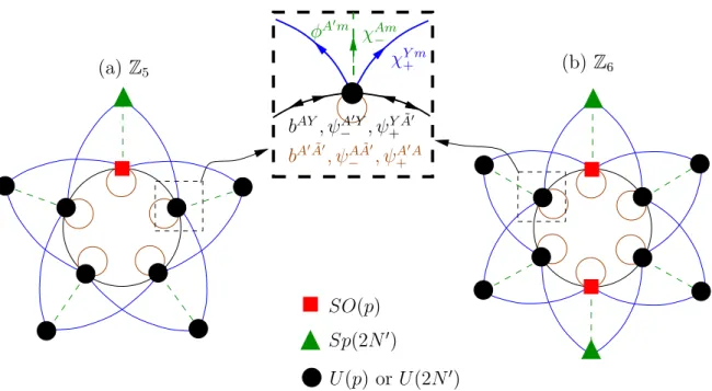
We are interested in finding the boundary CFT that corresponds to this setup. We propose that it is given by a two-dimensional (0,4) sigma model arising on the Higgs branch of an orbifolded ADHM model. This generalises the models introduced in [183, 59].

To check this proposal, we compare the left- and right-moving central charges of the infrared conformal field theory to those predicted by the worldsheet model. More precisely, we need to flow the ADHM model, which we know in the UV, to its infrared fixed point.

One can show however that there is no renormalisation group flow [138], so that one can simply count the massless degrees of freedom in the UV. Our counting is then in perfect agreement with the prediction from the worldsheet side.

Pure gravity and extremal CFTs

Chapters 5 and 6 deal with a very specific kind of dual CFT, so-called extremal CFTs.

Their motivation comes from the analysis of Witten concerning pure gravity in AdS3 [185].

In particular, he proposes the existence of extremal dual theories, which could serve as dual CFTs to pure gravity. We will give arguments that such extremal theories cannot exist.

Let us first introduce some concepts needed later on. By pure gravity we mean that the theory contains only the bare essentials necessary, and no additional matter or gauge fields. The dual CFT then also only contains a very limited number of states, which is why we call it extremal.

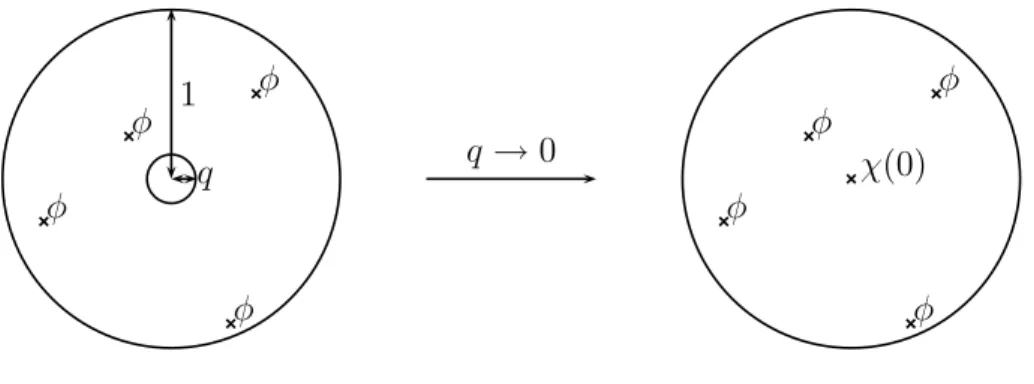
Our arguments will make use of modular properties of partitions functions. The partition function orcharacter of a CFT is defined as

χ_M(q) = Tr_M(q^L⁰^−c/24) ,

where the trace is taken over all states of the representationM of the theory. In particular, χM counts the number of states at each level. Physically, it corresponds to the zero-point function on the torus. The torus remains invariant under transformations of the modular group SL(2,Z). All physical quantities that depend on τ should thus also be invariant under modular transformations. This places strong constraints on the partition function.

Witten then suggested that the boundary theories that correspond to pure gravity should be holomorphically factorising extremal bosonic conformal field theories of central chargec= 24k. The integerkis proportional to the AdS radius of the spacetime geometry.

We are mainly interested in the case of large k where the curvature becomes weak.

There are only two kinds of excitations in pure gravity: perturbative excitations and black holes. The perturbative excitations are identified with Virasoro descendants of the vacuum following [23] while the BTZ black holes correspond to the new primaries. Since black holes are parametrically heavy there is a large gap from the vacuum to the first nontrivial primary. Extremality then means that the partition function of the boundary CFT is as close as possible to the Virasoro character of the vacuum, i.e. that it starts to differ from it only at a high level.

(18)

The above constraints specify the potential character of such meromorphic conformal field theories uniquely. Fork = 1, the resulting character is the j invariant minus 744,

j(q)−744 = 1

q + 196884q+ 21493760q²+. . . .

To see that this theory is extremal note that the coefficient of q⁰ is zero, so that there are no states at level 1. The corresponding conformal field theory is the famous Monster theory [83, 20]. Fork≥2 one can write down similar partition functions, but an explicit realisation of these theories is so far not known. In chapter 5 we investigate if theories corresponding to these characters can exist at all. Following [91], we use null vectors and their associated modular differential equations to find consistency conditions for such theories which go beyond the existence of the partition function.

More specifically, if a null vector is inserted in the trace over any representation, one obtains a differential equation which annihilates the character. Moreover, the form of this differential equation is independent of the representation, i.e. the same equation annihilates all characters of a theory. The order of the equation depends on the level of the null vector. On the other hand, if one knows all the characters of a theory, one can by inspection find a modularly covariant differential equation which annihilates all of them.

In chapter 5 we show the converse, i.e. that each such equation must come from at least one null vector. It is possible, however, that the level of the null vectors is higher than the order of the differential equation, so that we cannot draw a direct conclusion on its conformal weight. On the other hand, the bigger the difference between the two, the more null vectors are needed. As long as the theory does not have an extremely high number of null vectors, the differential equation has approximately the same order as the level of the null vector.

For the proposed extremal theories this leads to a contradiction for k ≥42, since the differential equation predicts null vectors at a level where they are excluded by extremality [91].

In chapter 6 we take a step back and perform the analogue of the analysis of [185], only this time for the N = (2,2) supersymmetric case. Again, we only allowN = (2,2) descendants of the vacuum and primary fields which correspond to BTZ black holes. BTZ black holes in this setup are characterised by their mass and charge, which we identify on the CFT side with their conformal weight andU(1) charge. From classical supergravity, we know that there exists a so-called cosmic censorship bound: if the chargeℓ of a black hole is too big compared to its mass n, then the solution has a singularity which lies outside its event horizon. To avoid this, we allow only black holes for which

4mn−ℓ² ≥0 ,

where m is the analogue of k in the bosonic case, i.e. the AdS radius. The cosmic censorship condition is the analogue of the requirement that the bosonic black holes be parametrically heavy, that is it restricts the kind of primary fields that can be introduced in the theory.

As was mentioned before, theN = 2 superconformal algebra has more structure than the Virasoro algebra; in particular, it contains aU(1) currentJ. The zero modeJ0 is then

(19)

an additional element of the Cartan subalgebra and can thus be inserted in the character much in the same way as L0. This construction leads to the elliptic genus of the theory, the main object of interest in our analysis. The elliptic genus thus not only contains information on the weight of states, but also on their charges.

Mathematically, the elliptic genus is a so-called weak Jacobi form. Its Fourier expansion is given by

χ(q, y) =X

n≥0

X

ℓ∈Z

c(n, ℓ)qⁿy^ℓ ,

and it has nice transformation properties under modular transformations and spectral flow. The space of all possible weak Jacobi form is a ring generated by four generators.

The set of all terms for which 4mn−ℓ² <0 are called the polar part of χ. Note that this coincides with the cosmic censorship bound introduced above.

By this argument, we know that BTZ black holes cannot change the number of states below the cosmic censorship bound. This means that the coefficients of the polar terms of χ are fixed by the N = 2 vacuum character. The number of polar terms however is bigger than the number of allowed weak Jacobi forms, or, to put it another way, the system of equations so obtained is overdetermined. Generically, we thus do not expect an extremal elliptic genus to exist; using a rather technical analytical argument, one can show that for large AdS radii this is indeed true. The only genera that do exist are in fact m= 1,2,3,4,5,7,8,11,13.

On the other hand, one can show that an elliptic genus exists for all curvatures if one relaxes the cosmic censorship bound somewhat. This leads to the notion of near-extremal CFTs. In particular, since the original form of the bound is taken from a purely classical calculation, one cannot rule out that quantum corrections could modify the bound in just the right way to make the theory work. The N = 4 case however, for which one does not expect any quantum correction, does not seem to work much better. Our arguments thus give strong indications that pure supergravity theories are inconsistent.

Chapters 1 and 2 are based on [79] and [80] written in collaboration with S. Freden- hagen and M. Gaberdiel. Chapter 3 is based on [134]. Chapter 4 is based on [121], written in collaboration with S. Hohenegger and I. Kirsch. Chapter 5 is based on [94] written in collaboration with M. Gaberdiel. Chapter 6 is based on [93] written in collaboration with M. Gaberdiel, S. Gukov, G. Moore, and H. Ooguri.

(20)

(21)

Part I

RG flows on the worldsheet

(22)

(23)

Chapter 1 Bulk-induced boundary perturbations

1.1 Overview

In the introduction we have seen that in CFT the closed string moduli space is described by the exactly marginal bulk perturbations. A necessary condition for a bulk field to be exactly marginal is that it has conformal weight (1,1), and that its three-point self- coupling vanishes [130, 30]. This condition was derived for conformal field theories without boundary, but in the presence of a D-brane, the situation changes. Indeed, a marginal bulk operator that is exactly marginal in the bulk theory may cease to be exactly marginal in the presence of a boundary.

The simplest example where this phenomenon occurs, is the theory of a single free boson compactified on a circle. For this theory the full moduli space of conformal D- branes is known [97, 125] (see also [85, 168]). It depends in a very discontinuous manner on the radius of the circle, which is one of the bulk moduli. We always have the usual Dirichlet and Neumann branes, but if the radius is a rational multiple of the self-dual radius, the moduli space contains in addition a certain quotient of SU(2). On the other hand, for an irrational multiple of the self-dual radius the additional part of the moduli space is just a line segment. The bulk operator that changes the radius is exactly marginal for the bulk theory, but in the presence of certain D-branes it is not. In particular, it ceases to be exactly marginal if we consider a rational multiple of the self-dual radius and a D-brane which is neither Dirichlet or Neumann, but which is associated to a generic group element g of SU(2). If we change the radius infinitesimally, it is generically not a rational multiple of the self-dual radius any more, and thus the brane associated to g is no longer conformal.

In order to understand the response of the system to the bulk perturbation we set up the renormalisation group (RG) equations for bulk and boundary couplings. This can be done quite generally, and we find that whenever certain bulk-boundary coupling constants do not vanish, the exactly marginal bulk perturbation is not exactly marginal in the presence of a boundary, but rather induces a non-trivial RG flow on the boundary. In particular, this therefore gives a criterion for when an exactly marginal bulk deformation

(24)

is also exactly marginal in the presence of a boundary.

For the above example of the free boson, the resulting RG flow equations can actually be studied in quite some detail. We find that upon changing the radius the resulting flow drives the brane associated to a generic group elementg(that only exists at rational radii) to a superposition of pure Neumann or Dirichlet branes (that always exist). Whether the end-point is Dirichlet or Neumann depends on the sign of the perturbation,i.e. on whether the radius is increased or decreased. At the self-dual radius, the theory is equivalent to the SU(2) WZW model at level 1, and the analysis can be done very elegantly. In this case we can actually give a closed formula for the boundary flow which is exact in the boundary coupling (at first order in the bulk coupling).

Some of these results can be easily generalised to arbitrary current-current deformations of WZW models at higher level and higher rank. While we cannot, in general, give an explicit description of the whole flow any more, we can still describe at least qualitatively the end-point of the boundary RG flow.

1.2 CFTs with boundaries

Let us give a very brief introduction to CFTs with boundaries, fleshing out some of the material mentioned in the introduction. More detailed introductions to conformal field theory are for example [48, 105]. As mentioned before, we can separate the energy- momentum tensor T into its holomorphic part T(z) and its anti-holomorphic part ¯T(¯z).

We can then expandT(z) in terms of its modes, T(z) = X

n∈Z

Lnz⁻ⁿ⁻^h . (1.2.1)

The Virasoro generatorsLn satisfy the Virasoro algebra, [Lm, Ln] = (m−n)Lm+n+ c

12m(m²−1)δm+n . (1.2.2) Conformal symmetry requires that all states of the theory decompose into representations of the Virasoro generatorsLn. So-called primaryfields are fields which have good transformation properties under conformal transformations. In particular, a primary field φ(z,z) transforms as¯

φ(z,z)¯ 7→(f^′(z))^h f¯^′(¯z)h^¯

φ(f(z),f(¯¯z)) , (1.2.3) whereh and ¯hare the (holomorphic and anti-holomporphic) conformal weight ofφ. Fur- ther states, the so-called descendants, can be obtained by acting with Virasoro generators on primary fields. Using conformal symmetry, one can reduce correlation functions of descendants to correlation functions of primary fields.

Let us turn to CFTs with boundaries. It is often convenient to describe such theories as living on the upper half planeH+ of the complex plane; the boundary is then the real axis z = ¯z. Boundary conditions are imposed by relating left-moving fields to right-moving

(25)

fields on said axis. If the theory is to remain conformal, it is in particular necessary to identify

T(z) = ¯T(¯z) forz = ¯z . (1.2.4) It is then possible to analytically continueT(z) to the lower half plane using the prescription

T(z) =

T(z) Imz ≥0

T¯(z) Imz <0 . (1.2.5)

This means that we have essentially reduced the problem of a full CFT on the upper half plane to the left-moving sector of a CFT on the entire complex plane.

The above description of boundary conditions is the open string picture. It is often convenient to change to the closed string picture by performing a modular S transform on the worldsheet. In this case, for instance the 1-loop diagram of an open string whose endpoints lie on two D-branes becomes the diagram of a closed string propagating from an initial state to a final state. This state is the so-called boundary state ||Bii. In this language, the condition for conformal invariance is then

(Ln−L¯_−n)||Bii= 0 . (1.2.6) Additional symmetries of the theory are described by its chiral algebra, i.e. by fields which only have a left- or right-moving component. In a theory with boundary such a symmetry is preserved if on the boundary the left- and right-moving chiral fields are related by an automorphism, the so-called gluing map. Many of these questions will be discussed in more detail in chapter 2.

1.3 The renormalisation group equation

In this section we shall analyse the RG flow involving bulk and boundary couplings.

Bulk perturbations by relevant operators for conformal field theories with boundaries have been considered before in the context of integrable models starting from [37] and further developed in [174, 88, 102]. In particular, these flows have been studied using (an appropriate version of) the thermodynamic Bethe ansatz (see e.g. [141, 144, 56, 57, 54]), in terms of the truncated conformal space approach (see e.g. [56, 57, 55]), and recently by a form factor expansion [13, 34].

LetS^∗ be the action of a conformal field theory on the upper half plane. We denote the bulk fields by φi, and the boundary fields by ψj. Their operator product expansions are of the form

φi(z)φj(w) = |z−w|^h^k^−hⁱ^−h^jCijkφk(w) +· · · , (1.3.7) ψi(x)ψj(y) = (x−y)^h^k⁻^hⁱ⁻^h^jDijkψk(y) +· · · , (1.3.8) where Cijk and Dijk are the bulk and boundary OPE coefficients, respectively. We are interested in the perturbation of this theory by bulk and boundary fields,

S =S^∗+X

i

λ˜i

Z

φi(z)d²z+X

j

˜ µj

Z

ψj(x)dx . (1.3.9)

(26)

Introducing the length scale ℓ, we define dimensionless coupling constants λ_i and µ_j by λ˜i =λiℓ^h^φi⁻² , µ˜j =µjℓ^h^ψj⁻¹ . (1.3.10) Note that we do not assume here thatφ_i and ψ_j are marginal operators.

Let h. . .i denote the correlators in the unperturbed theory; the perturbed correlators are then defined as

hφ1(z1,z¯1)· · ·φn(zn,z¯n)iλ = hφ₁(z₁,z¯₁)· · ·φ_n(z_n,z¯_n)e⁻^∆^Si

he⁻^∆^Si , (1.3.11)

and similarly for correlators involving boundary fields. The expression on the right hand side is divergent and has to be regularised. If we expand the exponential in powers ofλ_i and µj, we get terms of the form

λ^l₁¹· · ·µ^m₁¹· · · l1!· · ·m1!· · ·

Y

i

ℓ^(h^φi^−2)lⁱY

j

ℓ^(h^ψj^−1)m^j

× Z

hφ1(z₁¹)φ1(z₂¹)· · ·φ2(z₁²)· · ·ψ1(x¹₁)· · · iY

d²z_kⁱ Y

dx^j_k . (1.3.12) Since (1.3.12) is divergent, we need to specify a regularisation scheme. The most straight- forward one is to cut out little disks around operator insertions by introducing an UV cutoff ℓ. More precisely, the prescription is

|z_kⁱ −z_kⁱ^′′|> ℓ , |x^j_k−x^j_k^′′|> ℓ , Imz > ℓ

2 . (1.3.13)

The parameter ℓ thus appears in (1.3.12) both explicitly as powers in h, and implicitly through the range of integration. In chapter 3 we will rederive the RG equations using a different regularisation scheme somewhat resembling dimensional regularisation; but for the moment, we shall use (1.3.13).

Following [30] we now consider a change of the scale ℓ, ℓ → (1 +δt)ℓ, and ask how the coupling constants have to be adjusted so as to leave the free energy unchanged. The explicit dependence of the expression (1.3.12) onℓ leads to a change in λi and µj by

λi →(1 + (2−hφi)δt)λi ,

µj →(1 + (1−hψj)δt)µj . (1.3.14) The implicit dependence of (1.3.12) on ℓ through the UV prescription (1.3.13) gives rise to an additional change of the coupling constants. From the first inequality in (1.3.13), which controls the UV singularity in the bulk operator product expansion, we obtain the equation δλk = πCijkλiλjδt [30]. A similar calculation gives δµk = Dijkµiµjδt (see for example [3]) for the contribution from the boundary operator product expansion (the second inequality). Finally we have to consider the contribution from the third inequality which controls the singularity that arises when a bulk operator approaches the boundary.

When we scaleℓ by (1 +δt) we change the integration region of a bulk operator by a strip

(27)

parallel to the real axis of width ℓ δt/2. This changes the expression (1.3.12) by terms of the form

−λiℓ^h^φi⁻² Z

dx

Z ℓ/2+ℓδt/2 ℓ/2

dyh· · ·φi(z)· · · i, (1.3.15) where we have written z = x+iy. In order to evaluate this contribution, we use the bulk-boundary operator product expansion

φi(z,z) = (2y)¯ ^h^ψj^−h^φiBijψj(x) +· · · , (1.3.16) where Bij is the bulk-boundary OPE coefficient that depends on the boundary condition in question. The change of the free energy described by (1.3.15) is then

−λiℓ^h^φi⁻² Z

dxℓ δt

2 Bijℓ^h^ψj⁻^h^φih· · ·ψj(x)· · · i=−1

2Bijℓ^h^ψj⁻¹λiδt Z

dxh· · ·ψj(x)· · · i (1.3.17) which can be absorbed by a shift of δµj = ¹₂λiBijδt. Collecting all terms, we thus obtain the RG equations to lowest order

λ˙k = (2−hφk)λk+πCijkλiλj +O(λ³) , (1.3.18)

˙

µk = (1−hψk)µk+ 1

2Bikλi+Dijkµiµj +O(µλ, µ³, λ²) . (1.3.19) The flow of the bulk variablesλk in (1.3.18) is independent of the boundary couplingsµk

on the disc. The RG flow in the bulk therefore does not depend on the boundary condition whereas the bulk has significant influence on the flow of the boundary couplings. Note that the terms we have written out explicitly are independent of the precise details of the UV cutoff (if the fields are marginal). Higher order corrections, on the other hand, will depend on the specific regularisation scheme.

Suppose now that φi is an exactly marginal bulk perturbation. The perturbation by φ_i is then exactly marginal in the presence of a boundary if the bulk boundary coupling constants Bik vanish; this has to be the case for all boundary fields ψk (except for the vacuum) that are relevant or marginal, i.e. satisfy hψk ≤1. Obviously, switching on the vacuum on the boundary just leads to a rescaling of the disc amplitude; for irrelevant operators, on the other hand, the flow is damped by the first term of (1.3.19), and thus the bulk perturbation only leads to a small correction of the boundary condition.

The above condition is the analogue of the usual statement about exact marginality:

a necessary condition for a marginal bulk (boundary) operator to be exactly marginal is that the three point couplingsCiik (Diik) vanish for all marginal or relevant fieldsφk (ψk), except for the identity (see for example [130, 30, 168]).

If the bulk boundary coefficient Bik does not vanish for some relevant or marginal boundary operator ψk, the corresponding boundary coupling µk starts to run, and there is a non-trivial RG flow on the boundary. The bulk couplings λi are not affected by the flow ( ˙λi = 0), and we can thus interpret it as a pure boundary flow in the marginally deformed bulk model. From that point of view it is then clear that the flow must respect the g-theorem [3, 86]. In particular, the g-function of the resulting brane is smaller than

(28)

that of the initial brane. This is in fact readily verified for the examples we are about to study.

In chapter 2, we will rederive the above results using a somewhat different approach, namely by analysing symmetries of the theory. As a special case, one can then check under which conditions the conformal symmetry survives, and obtains the same result — see 2.3.1 for more details.

1.4 The free boson theory at the self-dual radius

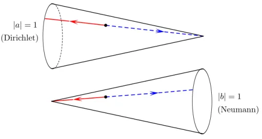
As an application of these ideas, we now consider the example of the free boson theory at c = 1. We shall first consider the theory at the critical radius, where it is in fact equivalent to the WZW model ofsu(2) at level 1. For this theory all conformal boundary states are known [98], and are labelled by group elementsg ∈SU(2) (for earlier work see also [26, 166]).

Suppose that we are considering the boundary condition labelled byg ∈SU(2), where we write

g =

a b^∗

−b a^∗

, (1.4.1)

and a andb are complex numbers satisfying|a|²+|b|² = 1. (Geometrically, SU(2) can be thought of as a product of two circles — see figure 1.1.) We shall choose the convention that the brane labelled byg satisfies the gluing condition¹

g J_m^αg⁻¹+ ¯J_−m^α

||gii= 0 , (1.4.2)

where J^α are the currents of the WZW model (the corresponding Lie algebra generators will be denoted byt^α). We shall furthermore use the identification thatg diagonal (b = 0) describes a Dirichlet brane on the circle, whose position is given by the phase of a;

conversely, if g is off-diagonal (a= 0), the brane is a Neumann brane, whose Wilson line on the dual circle is described by the phase of b.

1.4.1 Changing the radius

We want to consider the bulk perturbation by the field Φ =J³J¯³ , where t³ = 1

√2

1 0 0 −1

. (1.4.3)

This is an exactly marginal bulk perturbation that changes the radius of the underlying circle. With the above conventions, the perturbationλΦ with λ >0 increases the radius, whileλ < 0 decreases it. At any rate, the perturbation by Φ breaks thesu(2) symmetry down tou(1). However, in the presence of a boundary, the bulk perturbation is generically not exactly marginal any more. This is implicit in the results of [97, 125, 85] since the set of possible conformal boundary conditions is much smaller at generic (irrational) radius

1Note that the labelling differs from the one used in [97].

(29)

relative to the self-dual case. Here we want to study in detail what happens to a generic boundary condition under this bulk deformation.

Even before studying the detailed RG equations that we derived in the previous section, it is not difficult to see that the above deformation is generically not exactly marginal.

In particular, we can consider the perturbed one-point function of the field Φ in the presence of the boundary. To first order, this means evaluating the 2-point function

λ Z

H+

d²zh(J^αJ¯^α)(z) (J^αJ¯^α)(w)i, (1.4.4) where the label α = 3 is not summed over. Using the usual doubling trick [28] this amplitude can be expressed as a chiral 4-point function, where we have the fields J^α at z and w, and the ‘reflected’ fields J^β ≡gJ^αg⁻¹ at ¯z and ¯w.

The chiral correlation functions of WZW models at level k can be calculated using the techniques of [84, 92]. Let t^α, α = 1, . . . ,dim(g), be the Lie algebra generator (corresponding to J^α) in some representation; we choose the normalisation

Tr(t^αt^β) =k δ^αβ . (1.4.5)

To evaluate hJ^α¹(z1)· · ·J^αⁿ(zn)i, consider then all permutations ρ ∈ Sn that have no fixed points; this subset of permutations is denoted by ˜Sn. Each such ρ can be written as a product of disjoint cycles

ρ=σ1σ2· · ·σM . (1.4.6) To each cycle σ = (i₁i₂· · ·i_m) we assign the function

fσ^αⁱ¹^···α^im(zi1, . . . , zim) =− Tr(t^αⁱ¹ · · ·t^α^im)

(zi1 −zi2)(zi2 −zi3)· · ·(zim−zi1) , (1.4.7) and to each ρthe productfσ1· · ·fσM. The correlation function is then given by summing over all permutations without fixed points,

hJ^α¹(z1)· · ·J^αⁿ(zn)i= X

ρ∈S˜n

fρ . (1.4.8)

In (1.4.4), ρ is either a 4-cycle or consists of two 2-cycles. In the latter case we get the terms

(Tr(t^αt^β))²

|z−z¯|²|w−w¯|² +(Tr(t^αt^β))²

|z−w¯|⁴ + Tr(t^αt^α)Tr(t^βt^β)

|z−w|⁴ . (1.4.9) Integration over the upper half plane gives (divergent) contributions proportional to

|w−w¯|⁻², which can be absorbed in the renormalisation of J^α. The six terms that come from the six different 4-cycles give a total contribution of

− Tr([t^α, t^β]²)

(z−z)(w¯ −w)¯ |z−w¯|² . (1.4.10) Set w=i|w| and z =x+iy. The resulting integral over the upper half plane is logarith- mically divergent for y→0. Introducing an ultraviolet cutoff ǫ, we get

Z

R

dx Z _∞

ǫ

dy 1 2iy2i|w|

1

x²+ (y+|w|)² = π

4|w|²logǫ− π

8|w|² log|w|²+O(ǫ). (1.4.11)

(30)

|a|= 1 (Dirichlet)

|b|= 1 (Neumann)

Figure 1.1: The moduli space of D-branes on the self-dual circle,SU(2), can be described as a product of two circles S¹ (given by the phases of a and b in (1.4.1)) fibred over an interval where|a|runs between 0 and 1, and|a|²+|b|² = 1. The ends of the interval where one of the circles shrinks to zero describe Dirichlet and Neumann branes, respectively.

If we start with a generic boundary condition and increase (decrease) the radius, the boundary condition will flow to a Dirichlet (Neumann) boundary condition.

The first term has the right w dependence to be absorbed by a suitable renormalisation ofJ^α. The second term, however, pushes the conformal weight away from (1,1). Thus, if J^α is to be exactly marginal, the expression Tr([t^α, t^β]²) must vanish.

In the case above Tr([t^α, t^β]²) equals

Tr([t³, g t³g⁻¹]²) = −8|a|²|b|² . (1.4.12) This only vanishes if either|a|= 0 or |b|= 0; the corresponding boundary conditions are therefore either pure Dirichlet or pure Neumann boundary conditions. This ties in with the expectations based on the analysis of the conformal boundary conditions since only pure Neumann or Dirichlet boundary conditions exist for all values of the radius.

The argument above can also be used in the general case to derive a necessary criterion for when a bulk deformation is exactly marginal in the presence of a boundary. It is not difficult to see that it leads to the same criterion as the one given in section 1.3.

1.4.2 The renormalisation group analysis

Now we want to analyse what happens if g does not describe a pure Neumann or pure Dirichlet boundary condition. In particular, we can use the results of section 2 to understand how the system reacts to the bulk perturbation byλΦ.

In order to see how the boundary theory is affected by the perturbation we have to compute the bulk boundary OPE of the perturbing field Φ. There are no relevant boundary fields (except the vacuum), and the marginal fields are all given by boundary

(31)

currents J^γ. We can thus determine the bulk boundary OPE coefficient B_Φγ from the two-point function

hJ^γ(x)(J³J¯³)(z)i=BΦγ|z−z¯|⁻¹|x−z|⁻² , (1.4.13) which – employing the general formula (1.4.8) – leads to

BΦγ =−iTr(t^γ[t³, g t³g⁻¹]). (1.4.14) We see that the only boundary field that is switched on by the bulk perturbation is the current J^γ whose (hermitian) Lie algebra generator t^γ is proportional to the commutator [t³, g t³g⁻¹]. The normalised t^γ is given by

t^γ = i

√2

0 −e^iχ e^−iχ 0

with a b^∗ =|ab|e^iχ . (1.4.15) Its relation to the commutator is

−i[t³, g t³g⁻¹] =−i

0 −2ab^∗ 2a^∗b 0

=B t^γ , (1.4.16)

where the bulk boundary coefficient B =BΦγ is given by B =−2√

2|a| |b| . (1.4.17)

The boundary current proportional to t^γ modifies the boundary condition g by δg =i t^γg = 1

√2



−a_|^|^b_a^|_| b^{∗ |}_|^a_b^|_|

−b^|_|^a_b_|^| −a^{∗ |}_|_a^b^|_|



 . (1.4.18)

This leaves the phases of a and b unmodified, but decreases the modulus of a while increasing that of b.

Since the operators are marginal, the renormalisation group equation to lowest order in the coupling constants (1.3.19) is now

˙ µ= 1

2B λ+O(µλ, µ², λ²), (1.4.19) where µis the boundary coupling constant of the fieldJ^γ. Thus if the radius is increased (λ >0),µbecomes negative, and the boundary condition flows to the boundary condition with b = 0 — the resulting brane is then a Dirichlet brane whose position is determined by the original phase of a. Conversely, if the radius is decreased (λ < 0), µ becomes positive, and the boundary condition flows to the boundary condition with a = 0. The resulting brane is then a Neumann brane whose Wilson line is determined by the original value of the phase of b (see figure 1.1). This is precisely what one should have expected since for radii larger than the self-dual radius, only the Dirichlet branes are stable, while for radii less then the self-dual radius, only Neumann branes are stable.