Methodical aspects of urinary metabolomics by liquid chromatography - mass spectrometry

metabolomics by liquid chromatography - mass spectrometry

Dissertation

zur Erlangung des Doktorgrades der Naturwissenschaften (Dr. rer. nat.) an der Naturwissenschaftlichen Fakultät IV

-Chemie und Pharmazie- der Universität Regensburg

vorgelegt von Franziska C. Vogl

aus Eggenfelden im Jahr 2019

Diese Doktorarbeit entstand in der Zeit von Juli 2012 bis August 2018 am Insti- tut für Funktionelle Genomik an der Universität Regensburg.

Die Arbeit wurde angeleitet von Prof. Dr. Peter J. Oefner.

Promotionsgesuch eingereicht am: 12.04.2019

Für meine Eltern

Danksagung

So, nun ist es soweit und ich darf endlich all denjenigen Menschen meinen Dank aussprechen, die maßgeblich dazu beigetragen haben, dass ich diese Arbeit fertig stellen konnte.

An erster Stelle gilt mein Dank Prof. Dr. Peter J. Oefner, der mir es ermöglicht hat, an seinem Lehrstuhl diese interessante Arbeit zu verfassen. Vielen Dank auch für die Übernahme des Erstgutachtens. Die Möglichkeit auf internationalen Konferenzen Erfahrung sammeln zu dürfen, sowie die fachliche Begleitung und Unterstützung habe ich sehr geschätzt.

Vielen Dank auch an Prof. Dr. Frank-Michael Matysik, der sich bereitwillig als Zweitgutachter zur Verfügung gestellt hat.

PD Dr. Katja Dettmer-Wilde möchte ich danken für die Bereitschaft als Dritt- prüfer und die fachliche Betreuung. Danke für deine Geduld, deine konstruktive Kritik und dein offenes Ohr in jeder Lebenslage. Mit deinem unendlichen GC/LC-MS Wissen hattest du immer einen passenden Tipp parat, der mir wei- tergeholfen hat. Ohne dich, hätte ich nicht gewusst, dass „nach zu, ab kommt“

und was der Unterschied zwischen Schraubenschlüssel und Schraubenzieher ist. Es hat wahnsinnig Spaß gemacht, mit dir gemeinsam am Maxi zu schrau- ben und dabei manchmal sogar alle Teile wieder richtig verbaut zu bekommen.

Nur die Namensgebung deiner Spielgefährten (Georg, Metti, etc.) war am An- fang etwas verwirrend für mich. Unvergesslich bleibt für mich auch „Pinky and the Brain“ und deine CSI Einlage.

Des Weiteren möchte ich Prof. Dr. Antje Baeumner danken für die Übernah- me des Prüfungsvorsitzes.

Ein ausdrücklicher Dank geht auch an die Nachwuchsförderung der Universität Regensburg für die Promotionsabschlussförderung, die ich für die Fertigstellung meiner Dissertation erhalten habe.

Bei Prof. Dr. Wolfram Gronwald, bedanke ich mich für die fachlich sehr kom- petenten Ratschläge und den Einblick in die Welt der NMR. An das gemeinsa- me Skifahren erinnere ich mich gerne zurück.

Für die gute Zusammenarbeit, die gemeinsame Publikation sowie den immer guten Informationsaustausch möchte ich Dr. Peggy Sekula recht herzlich dan- ken.

Es war mir eine Ehre Dr. Magda Waldhier kennen gelernt zu haben. Die ge- meinsamen Yogaabende waren immer sehr gesprächig und lustig. Und auch durch die Niederbayern Fraktion, bestehend aus Dr. Christian Wachsmuth und Raffaela Berger hab ich mich wie zu Hause gefühlt. Ihr wart meinem nie- derbayrischen Dialekt gewachsen und habt auch das besondere bayrische Lob

„basst scho“ richtig deuten können. Die entstandene und bis heute bestehende Freundschaft mit euch Dreien bedeutet mir sehr viel.

Ein besonderes Dankeschön auch an Dr. Helena Zacharias, Jochen Hoch- rein, Franziska Taruttis und PD. Dr. Julia Engelmann die mir bei jeglichen statistischen und programmier-technischen Problemen zur Seite standen.

Danke an „Pinky“ alias Nadine Nürnberger. Du warst unser farbiger Stern im sonst eher tristen Laboralltag. Leider hat es dich wieder in die Heimat gezogen.

Deine Geburtstagsparty mit Tortenschlacht ist jedenfalls legendär. Das Küken, Claudia Samol, hat jede Mittagspause zum spannenden Erlebnis gemacht. Als unermüdliche „Pippettöse“ und „Vorthexe“ war es toll mit dir im Labor zu arbei- ten, auch wenn die Aliquotierung der Urinproben nie enden wollte. Bei der gu- ten Seele, Lisa Ellmann, bedanke ich mich auch recht herzlich für die Hilfestel- lungen im Labor, vor allem für die Zeit, als ich nicht mehr ins Labor durfte und du meine etwas komplizierten Anweisungen interpretieren musstest.

Dem „PC-Betreuer vor Ort“ Christian Kohler möchte ich besonders Danken.

Du hast dich immer sofort um alle meine kleineren und auch größeren Compu- ter Probleme und Problemchen gekümmert. Und auch bei der Namensgebung deiner Tochter hast du alles richtig gemacht.

Meinen Kaffee Buddies Dr. Jörg Reinders und Dr. Yvonne Reinders, möchte ich auch noch danken. Ihr hattet immer Zeit für ein Gespräch, sowohl fachlicher als auch privater Art. Eure kulinarische Verpflegung war ein Highlight, in deren Gunst wir des Öfteren bei so manchen Grillpartys kamen.

Für das sonnige Gemüt, die heitere, aufbauende Art und auch dafür, dass du immer einen Übernachtungsplatz hattest, bedanke ich mich bei Elke Perthen.

Den beiden NMR-lern, Dr. Trixi von Schlippenbach und Dr. Philipp Schwarz- fischer, sowie den alten Hasen Dr. Nadine Assmann, Dr. Matthias Klein und Dr. Martin Almstetter, die mir vor allem am Anfang sehr geholfen haben, möchte ich danken.

Bei Dr. Thomas Stempfl und Dr. Christoph Möhle bedanke ich mich für das Asyl am Ende meiner aktiven Zeit am IFG. Mit euren Labordamen, Jutta Schipka und Susanne Schwab, waren so manche Mittagspausen im Nu vor- bei. Und auch die beiden Organisationstalenten Eva Engl und Sharon Peter- sen möchte ich noch dankend erwähnen.

Allen ehemaligen und aktiven Kollegen am IFG danke ich für die schöne und lehrreiche Zeit an die ich mich gerne erinnere.

Mein besonderer Dank geht an Marianne Felixberger. Nicht nur als Oma von Marie bist du immer für uns da. Du hast mir den Rücken frei gehalten und mich motiviert, damit ich diese Arbeit fertig stellen konnte. Danke für alles.

Meinen Eltern Gisela und Wolfgang Vogl, sowie meiner Lieblingsschwester Alexandra Lehner gebührt der größte Dank. Ohne euren Rückhalt hätte ich diese Arbeit nicht zu Ende gebracht. Kein Jammern und Klagen meinerseits war euch zu viel. Kein Weg zu weit, um mir zu helfen. Ihr habt mich bedingungslos unterstütz. Ihr könnt euch nicht vorstellen, wie wichtig das für mich war. Einer für alle und alle für einen!

Johannes und Marie, ihr seid mein Ein und Alles, mein Fels in der Brandung.

Ihr wart immer verständnisvoll, wenn ich mal wieder wegen meiner Doktorarbeit keine Zeit für euch hatte. Das hat mir manchmal das Herz gebrochen. Eure Lie- be war meine wichtigste Stütze, die mir geholfen hat, diese Arbeit abzuschlie- ßen. Ich freue mich riesig auf unser Familienleben zu viert und auf die Abend- teuer die noch auf uns warten.

An dieser Stelle möchte ich auch an einen sehr guten Freund erinnern, der viel zu früh von uns gegangen ist: Dr. Alexander Riechers. Ich kann es immer noch nicht fassen, dass du nicht mehr unter uns bist. Mir fehlen dein Lachen, deine immer fröhliche Art und die Gummibärchen, die du immer für alle bereit hattest. Wie gerne hätte ich diesen Moment mit dir geteilt und mit dir gefeiert.

Mit deiner unbändige Hilfsbereitschaft, deinem immensen Wissen und deiner liebe zur Wissenschaft, warst du immer ein Vorbild für mich. Alex, du fehlst mir!

1. Table of contents

1. Table of contents ... VIII 2. Abbreviations and Acronyms ... XI

3. Motivation... 16

4. Background ... 20

4.1 Metabolomics ... 20

4.1.1 Fingerprinting analysis ... 20

4.1.2 Profiling analysis ... 22

4.2 LC-MS based metabolomics in the study of chronic kidney disease ... 23

4.3 Data analysis of untargeted large scale metabolomic studies ... 28

4.3.1 Data processing ... 29

4.3.2 Data visualization and statistical analysis ... 30

4.4 Identification of metabolites by LC-MS analysis ... 32

4.4.1 Identification workflow ... 33

4.4.2 Concrete examples for LC-MS based identification ... 36

5. Experimental section ... 39

5.1 Materials ... 39

5.2 Sample preparation ... 39

5.3 Instrumentation... 39

5.3.1 HPLC-ESI-TOFMS ... 39

5.3.2 HPLC-ESI-QqQMS ... 40

5.3.3 Miscellaneous ... 41

5.4 Data analysis ... 41

5.4.1 Software ... 41

5.4.2 Calibration curves ... 42

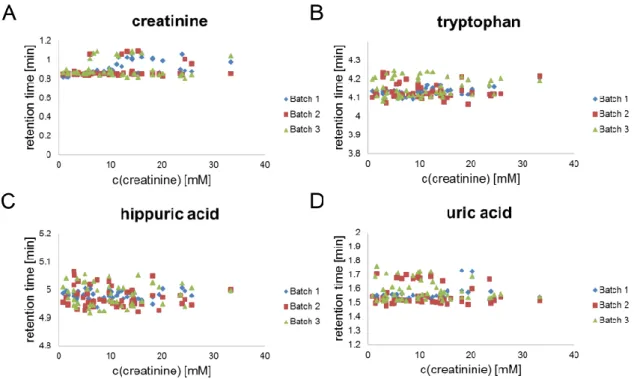
5.4.3 Retention time corrector (RTcorrector) ... 42

5.4.4 Bucket assigner ... 43

5.5 Validation methods ... 44

5.5.1 Hierarchical cluster analysis ... 44

5.5.2 Bland-Altman plot ... 45

6. Evaluation of dilution and normalization strategies to correct for urinary output in HPLC-HRTOFMS metabolomics ... 46

6.1 Introduction ... 46

6.2 Materials and Methods ... 48

6.2.1 Chemicals. ... 48

6.2.2 Urine specimens ... 48

6.2.3 Sample preparation ... 49

6.2.4 Creatinine quantification ... 50

6.2.5 Osmolality ... 51

6.2.6 LC-MS Analysis ... 51

6.2.7 Data Analysis ... 52

6.3 Results and Discussion ... 54

6.3.1 Creatinine Quantification ... 54

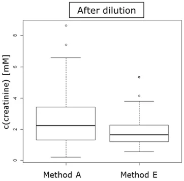
6.3.2 Basic characteristics of the first sample set ... 54

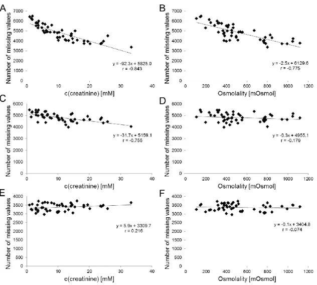
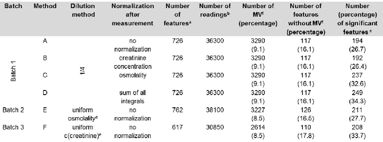
6.3.3 Effects of different dilution strategies on missing values . 57 6.3.4 Evaluation of different dilution strategies and normalization methods ... 59

6.3.5 Classification of a second sample set ... 66

6.3.6 Feature identification ... 67

6.3.7 Analysis of an independent patient cohort ... 68

6.4 Conclusions ... 72

7. Development of a quantitative LC-QqQMS method for renal disease- associated metabolites ... 73

7.1 Introduction ... 73

7.2 Experimentals ... 74

7.2.1 Chemicals ... 74

7.2.2. Solutions ... 75

7.2.3 Sample preparation ... 77

7.2.4 Instrumentation ... 78

7.3 Method validation ... 80

7.3.1 Quantification ... 80

7.3.2 Linear range, LOD and LOQ ... 81

7.3.3 Recovery and precision ... 81

7.4 Results and Discussion ... 82

7.4.1 Chromatographic separation and MS detection of analytes ... 82

7.4.2 Calibration ... 85

7.4.3 Spiking experiment ... 88

7.4.4 Application ... 90

7.5 Conclusions ... 94

8. Comparison of fingerprinting LC-HRTOF-MS and LC-QqQMS profiling data ... 96

8.1 Introduction ... 96

8.2 Materials and Methods ... 99

8.2.1 Calibration curves and urine sample preparation ... 99

8.2.2 Instrumentation ... 100

8.2.3 Data analysis ... 100

8.3 Results and Discussion ... 101

8.3.1 Comparison of calibration curves ... 101

8.3.2 Comparison of population based measurements on

targeted and untargeted platforms ... 104

8.4 Conclusions ... 110

9. Conclusion and Perspectives ... 112

10. References ... 114

11. Appendix ... 122

12. Publications and Presentations ... 126

12.1 Publications ... 126

12.2 Book Chapter ... 127

12.3 Oral Presentation ... 127

12.4 Poster Presentation ... 127

13. Summary... 128

14. Zusammenfassung ... 131

2. Abbreviations and Acronyms

AA Anthranilic acid

AER Albumin excretion rate AKI Acute chronic kidney injury CKD Chronic kidney disease CMT C-Mannosyltryptophan

CRE Creatinine

CRT Creatine

Da Dalton

DMX Dimethylxanthine

DN Diabetic nephropathy

eGFR Estimated glomerular filtration rate eGFRcr Estimated GFR based on creatinine ESI Electrospray ionization

ESRD End stage renal disease FDA Food and Drug Administration

GC Gas chromatography

GFR Glomerular filtration rate

GUA Guanidinoacetate

HAA Hydroxyanthranilic acid HIAA Hydroxyindolacetic acid

HIP Hippuric acid

HK Hydroxykynurenine

HMDB Human Metabolome Database

HPLC High performance liquide chromatography HRTOF High-resolution time-of-flight

HX Hypoxanthine

IAA Indole-3-acetic acid IDA Isotope dilution analysis ILA Indole-3-lactic acid INC Indole-3-carboxaldehyde IPA Indole-3-propionic acid IS Internal standard

IS 3-Indoxylsulfate

KA Kynurenic acid

KYN Kynurenine

LC Liquid chromatography LLOQ Lower limit of quantification LOD Limit of detection

LOQ Limit of quantification m/z Mass-to-charge ratio

MEL Melatonin

MG Methylguanine

MI 1-Methylinosine

MRM Multiple reaction monitoring

MS Mass spectrometry

MS/MS Tandem mass spectrometry

MX Methylxanthine

NA Nicotinic acid

NAM Nicotinamide

NIST National Institute of Standards and Technology NMR Nuclear magnetic resonance

PCA Principle component analysis

PLS-DA Partial least squares discriminant analysis

PSU Pseudouridine

QA Quinolinic acid

qMS Quadrupole mass spectrometry QqQ-MS Triple quadrupole MS

qTOF Quadrupole-Time-of-flight hybrid mass spectrometry RSD Relative standard deviation

S/N Signal to noise ratio

SER Serotonin

SIL-IS Stable isotope labeled internal standard SVM Support vector machines

TG Tiglylcarnitine

TIC Total ion current TOF Time of flight

TPO Tryptophol

TRP Tryptophan

TRY Tryptamine

UA Uric acid

ULOQ Upper Limit of quantification

XA Xanthurenic acid

XIC Extracted ion chromatogram

XT Xanthine

3. Motivation

Metabolomics aims at the holistic analysis of the qualitative and quantitative composition of low molecular weight compounds in biological systems.¹ The major goal is the determination of metabolites, quantitatively as well as qualita- tively, that differ between biological groups. This information is contributing to the understanding of the underlying biological mechanisms under investigation.

A common matrix for large scale metabolomics studies is urine since it is ob- tained non-invasively.^2,3 However, urinary output can vary widely due to various processes involved in the body’s water balance. The hydration is influenced by water uptake, loss of water due to respiration, perspiration and defecation³. As a result, variable urine amounts are excreted, which effects the metabolite con- centrations measured in the urine. Hence, untargeted LC-MS based metabo- lomics analyses of urine samples are challenging due to these biological vari- ances that are not necessarily related to the phenotype under investigation.

Consequently, to reveal the true biological variances, normalization strategies are necessary.⁴ Commonly, creatinine is utilized to normalize for urinary output.

Creatinine is an endogenous metabolite, produced at a constant rate and main- ly excreted by glomerular filtration.⁵ However, creatinine concentration can vary widely due to various factors, such as age, sex, body mass, health, diet or water intake.⁴ Alternatively, the osmolality, which is the molar sum of all solutes in urine, can be applied for correcting the urinary output because it reflects the urinary output more closely.⁴⁶ The common normalization procedure in metabo- lomics encompasses a uniform dilution of urine samples followed by a post- acquisition normalization to either creatinine concentration or to the sum of all integrals of each sample. Nevertheless, these normalization methods are una- ble to correct for column overloading, peak overlapping or ion suppression. Fur- thermore, a uniform dilution may result in failure to detect analytes in urine specimens of low concentration. Therefore, a normalization strategy is needed to overcome these shortcomings.

Chronic kidney disease (CKD) is a major public health concern affecting more than 10% of the population worldwide.⁷ Serum creatinine is the most commonly used clinical biomarker of renal dysfunction. However, there are important limi-

tations to its use. For example, it rises only after 50% of kidney function is al- ready lost. Additionally, tubular secretion of creatinine results in overestimation of renal function at lower glomerular filtration rates (GFR) and, as already men- tioned above, it reflects differences in muscle mass.⁸ Hence, serum creatinine concentrations can vary widely. Therefore, the estimation of GFR can be inac- curate. Cystatin C has been proposed as an alternative and more sensitive marker of eGFR.^9,10 However, it is metabolized by proximal tubular cells.¹¹ The ideal filtration markers for GFR estimation should exhibit no or only little net re- absorption or secretion in the nephron. This leads to the clinical necessity of additional markers for an early detection of CKD. Additionally, the underlying pathophysiological mechanisms are still not fully understood.¹² Sekula et al.

found that C-mannosyltryptophan and pseudouridine were strongly and repro- ducibly associated with eGRF and CKD in population-based studies.¹² There- fore, a quantitative method for further investigations was required for these me- tabolites.

For quantification of small molecules and metabolites, the triple quadrupole mass spectrometer in multiple reaction monitoring (MRM) mode has been the golden standard. However, with recent developments regarding the mass accu- racy, resolution and scan times, the relative quantification with a quadrupole Time-of-flight-mass spectrometer (qTOF-MS) in full scan mode is possible.¹³ Nevertheless, very little is known about the performance of quantification in full scan mode, also called untargeted screening, in biological matrices. Lu et al.

compared the performance of a triple quadrupole instrument in MRM mode to a TOF-MS in full scan mode for the analysis of 20 standard compounds (10 in positive ion mode, 10 in negative ion mode) at 5 different concentration levels and a cellular extract.¹³ However, they only showed the results for one standard compound. Therefore, a comparison of the absolute quantification via MRM mode and relative quantification via qTOF-MS in full scan mode in urine is needed.

Aim#1: Evaluation of strategies to reduce sources of variance in untarget- ed LC-MS based metabolomic analysis

As the sample preparation is one of the first steps in the analytical process, the first goal of this thesis was the optimization of the sample preparation of urine to correct for urinary output. For this purpose, the performance of different pre- and post-acquisition normalization methods to correct for urinary output in LC- MS based metabolic fingerprinting was systematically compared. As pre- acquisition methods, sample dilution to either a uniform creatinine concentra- tion, osmolality value, or using a constant factor were used. For the different post-acquisition normalization methods such as normalization to creatinine, os- molality and sum of all integrals, data were acquired with a constant 1:4 dilution.

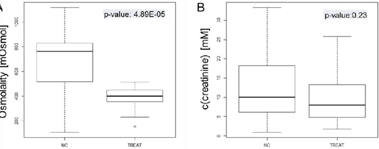
Urine specimens from patients with chronic kidney disease from two different epidemiological studies, namely the German chronic kidney disease study (GCKD)¹⁴ and the Trial to reduce cardiovascular events with Aranesp therapy (TREAT)¹⁵ study and healthy controls were chosen for evaluation of the differ- ent normalization and dilution strategies.

Aim#2: Development of a quantitative LC-QqQMS profiling method

The aim was the development of a sensitive and reliable quantitative profiling method for metabolites recently associated with renal disease, e.g. pseudouri- dine and C-mannosyltryptophan in order to further investigate these metabolites as potential markers. Moreover, seven metabolites identified as discriminating metabolites between patients suffering from CKD and healthy controls within the evaluation of normalization strategies together with the metabolites of the tryptophan pathway were also implemented in this method for further investiga- tions. The validated method was applied for the quantification of 383 urine and plasma samples from the GCKD study to analyze the fractional excretion.

Aim#3: Comparison of untargeted screening LC-qTOFMS and quantitative LC-QqQMS analysis

The goal was the comparison of fingerprinting LC-qTOFMS data and quantita- tive LC-QqQMS data of urine samples from the GCKD study. Since, the kidney function has a broad impact on circulation metabolite levels, untargeted metabolomics is a promising approach in nephrology research. However, the major drawback of untargeted (full scan) MS-based metabolomics is the semi- quantitative nature of the data.¹⁶ They are in arbitrary units and therefore cannot be compared across studies and further investigations e.g. in different matrices are difficult.¹⁷ In contrast, metabolic profiling methods provide absolute concen- trations for the investigated metabolites. Therefore, the generated data from the two different approaches were compared via Bland-Altman plots for a defined set of metabolites. Moreover, the lower limit of quantification (LLOQ), the upper limit of quantification (ULOQ), the linear range as well as the relative standard deviation (RSD) of the standard compounds for different concentrations were calculated and compared for both approaches.

4. Background

This chapter is focusing primarily on untargeted LC-MS based metabolomics.

4.1 Metabolomics

Metabolomics aims to investigate, qualitatively as well as quantitatively, all me- tabolites in a biological system simultaneously. Metabolites are low molecular weight compounds (<1000 Da) of organic or inorganic origin, which comprise mainly educts, intermediates or products of enzymatic biochemical reactions.¹⁸ Metabolomics encompasses the study of discriminative changes in metabolite profiles due to genetic modifications, physiological stimuli, environmental, nutri- tional or other factors ¹⁸. Hereby, the ultimate goal is the recognition of discrimi- native pattern rather than identifying all detected compounds.¹⁹

4.1.1 Fingerprinting analysis

Untargeted metabolomics, also called fingerprinting analysis, is considered to be the true “omics” approach.²⁰ Fingerprinting analysis enables a global snap- shot of the metabolic phenotype and therefore is also a valuable diagnostic tool.

19,21,22

The metabolome is the end-stage of the “omics”-cascade and hence re- flects genetic, disease, life style, as well as environmental responses. Metabolic profiles, obtained by analyzing metabolites, for instance, in body fluids such as serum or urine, provide additional information that cannot be obtained by inves- tigating the genotype, transcriptome, or even proteome. This additional knowledge can contribute to the achievement of personalized drug therapy.²² The analysis of reflective metabolite pattern enables therapy on a more person- alized level. Besides genotype variations, environmental influences like diet, which individually influence drug metabolism or toxicity, are also taken into ac- count.²³ Moreover, the characterization of metabolic networks by multiparamet- ric analysis may enable earlier diagnoses of some diseases.²⁴

As a large scale procedure, fingerprinting analysis covers a wide range of me- tabolites and enables a high number of experiments in a relatively short

time.^20,21 However, the varying molecular weight, hydrophobicity/hydrophilicity, acidity/basicity and boiling points of the metabolites represent major technical challenges. Technical platforms need to fulfill a variety of requirements like high accuracy, sensitivity and reproducibility.²⁰ Primarily, two different platforms are employed, which are either based on mass spectrometry (MS), coupled to a separation technique, or nuclear magnetic resonance (NMR). In principle, gas- chromatography-mass-spectrometry (GC-MS) and liquid-chromatography- mass-spectrometry (LC-MS) are the mainly used MS based platforms. Mass spectrometry based approaches have the potential not only to quantify metabo- lites with high sensitivity and selectivity but also to identify them. However, sample preparation is a crucial step for MS based analyzing techniques. Sam- ple preparation should be as simple as possible to minimize the loss of ana- lytes. Therefore, sample matrices that are compatible with the analytical tech- nique, are commonly only diluted and the dilution is adapted with respective to the sample concentration and the dynamic range of the MS. The coupling to a chromatographic separation technique reduces complexity of the matrix by add- ing the time scale as a further dimension. Moreover, it enables an isobaric sep- aration and achieves additional physicochemical information of the compounds.

Since GC-MS with electron ionization (EI) is a well-established method in metabolomics, robust protocols are available for fingerprinting analysis including maintenance, sample preparation, chromatographic evaluation and identifica- tion.²¹ The highly reproducible fragmentation with EI enables the implementa- tion of mass spectral libraries which facilitates metabolite identification. Never- theless, GC-MS is restricted to volatile analytes although chemical derivatiza- tion increases the range of detectable metabolites. Derivatization is a major bot- tleneck of GC-MS analysis because it can lead to different forms of derivatives for the same analyte, the derivatization reaction can be incomplete or it can lead to byproducts or degradation.²⁵ Furthermore, the additional sample preparation step may increase the analytical variance and can cause the loss of metabo- lites. However, there are correction methods, e.g. the derivatization of standard compounds and normalization methods, to overcome these shortcomings.²⁵ Nevertheless, GC-MS is considered to be the golden standard in metabolomics.

Yet, LC-MS has recently enjoyed a growing popularity as platform in metabo- lomics fingerprinting studies mostly because it can be applied to a larger diversi- ty of molecules^21,26,27. Moreover, there is no need for a derivatization step, which simplifies the sample preparation. The lower analysis temperatures allow a gentler metabolite handling.²⁸ However, metabolite identification is more diffi- cult due to the lack of comprehensive databases. Additionally, LC-MS meas- urements of complex matrices are hampered by ion suppression. The simulta- neous presence of multiple metabolites affects the ionization, which impedes quantification of these metabolites. Despite these difficulties recent enhance- ments in separation, ionization and mass accuracy, have contributed to a new level of performance. These new achievements made LC-MS a complimentary gold standard in metabolomics.

For the analysis of fingerprinting metabolomics data, the whole e.g. LC-MS chromatogram is exported. These signals yield characteristic patterns for each sample which can be tested for significantly different signals of different groups or can be used to classify the samples (see chapter 4.3). The significantly dis- criminating signals, also called features or markers, are then further investigat- ed and identified (see chapter 4.4.). Therefore, data complexity is reduced and only discriminatory metabolites are further analyzed and biologically interpreted.

Alternatively, NMR is applied as a comprehensive platform for fingerprinting analysis. Despite limitations in sensitivity, NMR provides a rapid, non- destructive, high throughput analysis with minimal sample preparation efforts.²⁸ Nevertheless, spectra are complex because most metabolites result in multiple signals that often overlap with signals from other metabolites. Therefore, me- tabolite identification is more complicated than with MS based approaches.

Moreover, a relatively large sample amount of a few hundred microliters is re- quired for NMR analysis. Due to the often restricted sample amount this is a major disadvantage of the NMR approach.

4.1.2 Profiling analysis

The second approach in metabolomics is called profiling or targeted analysis.

Thereby, defined sets of metabolites of a specific compound class or pathway are investigated quantitatively. For this purpose, analytical methods are special-

ly tailored to the respective metabolite set to be quantified. Moreover, sample preparation is normally more extensive than for fingerprinting analysis in order to minimize sample complexity prior to the measurements or to achieve a sam- ple pre-concentration for low abundant metabolites. Reference compounds with a known amount and an appropriate assortment of internal standards (IS) are applied to establish calibration curves for the quantification of the target ana- lytes. Instead of calibration curves, isotope dilution analysis (IDA) is also utilized for quantification (see Figure 4.1). Therefore, a known amount of the stable iso- tope labeled internal standard (SIL-IS) is added to the analyte to be quantified before the sample preparation procedure.²⁹ Hence, the losses of the analyte and SIL-IS are proportional and both are affected equally by ion suppression, matrix effects, injection variability and signal drifts. For the quantification the ratio of the peak area of the analyte to the SIL-IS is multiplied by the concentra- tion of the SIL-IS.²⁹ However, IDA is not only suited for quantification within a profiling analysis but it is also applicable for fingerprinting analysis (see chapter 6).

Figure 4.1: Isotope dilution analysis (IDA) exemplarily shown for the quantification of creatinine applying stable isotope labeled D3-creatinine. Adapted by permission from Springer, Practical Gas chromatography by Katja Dettmer-Wilde and Werner Engewald, Springer-Verlag Berlin Heidelberg 2014.²⁹

4.2 LC-MS based metabolomics in the study of chronic kidney disease

The kidneys play an important role in the acid-base balance, the regulation of plasma volume and hormone secretion, which all maintain vertebrate homeo-

stasis.³⁰ However, many kidney diseases can hamper these processes. Kidney diseases which persist over 3 months or longer are considered to be chronic (chronic kidney disease, CKD).³¹ Approximately 8-10% of the western popula- tion is affected by CKD.³² The clinical picture of CKD shows a progressive loss of the kidneys ability to filter potentially toxic compounds out of the blood into the urine.³³ Consequently, toxic compounds accumulate in the body, negatively affecting biological functions. Such compounds are also called uremic toxins.^33,34 Ninety uremic retention solutes were classified accordingly following the suggestion of the European uremic toxin work group.^33,35 This list was ex- tended in 2012 by Duration et al. who assigned 56 additional uremic toxins.³⁵ Diabetes mellitus and high blood pressure are the most prominent causes of CKD.³⁶ Patients suffering from diabetic mellitus are at increased risk of develop- ing diabetic nephropathy (DN). 30-40% of type 1 and 15-20% of type 2 diabetes mellitus patients have DN after 20 years. ^37,38

CKD is classified into five stages according to its severity. The classification is based on the estimated glomerular filtration rate (eGFR). The GFR is defined as the volume of plasma filtered by the glomeruli per unit of time.³⁹ It is equal to the Clearance Rate if the filtered substance is freely filtered and neither reabsorbed nor secreted by the kidney. Therefore, it can be measured using the clearance of filtration markers such as urinary creatinine. Urinary clearance can be calcu- lated applying the formula CL = U x V / P,^40,41 where U represents the urinary concentration, V the urinary flow rate, and P the plasma concentration.⁴⁰ GFR can also be estimated from serum levels of endogenous filtration markers (eGFR), such as serum creatinine or cystatin C, without the need of calculating the clearance.⁴⁰ A variety of different estimating equations are available using creatinine, all of them come with variable biases across populations and are imprecise.⁴⁰ Several estimation equations using cystatin C have also been pub- lished.⁴⁰ Calculation of eGFR based on cystatin C is not affected by muscle mass and diet. Hence, it is more reliable than calculations based on creatinine and not as strongly associated by sex, age and race.⁴⁰ On the downside, there is some evidence that shows cystatin C levels are influenced by tubular excre- tion.⁴⁰ Additionally, a combination of creatinine and cystatin C can also be used for the calculation of the eGFR.

Stage one of the CKD classification, as the mildest CKD class, shows only few symptoms (e.g. proteinuria) with a GFR < 90 mL/min/1.73 m², while stage five as the end stage displays severe symptoms (e.g. kidney failure) with a poor life expectancy if untreated (GFR < 15 mL/min/1.73 m²).³³ End stage renal disease (ESRD) either requires dialysis or renal replacement. In many kidney diseases, kidney damage can also be determined by albuminuria which is diagnosed based on urinary albumin excretion rate (AER).^31,42

Kidney disease and its associated metabolites were investigated with markedly

‘low-tech’ methodologies by physicians since the Middle Ages.⁴³ At that time, color, smell and taste of urine were applied to diagnose and specify renal dis- ease. Nowadays, clinical markers such as serum creatinine have been estab- lished for the detection of CKD. ⁴³ While classical assays, like colorimetric (Jaffe reaction) or enzymatic assays,⁴⁰ are still the gold standard in routine diagnos- tics, rapid improvements in analytical techniques made especially LC-MS a popular tool in the search for clinical markers. However, the sensitivity of these markers (e.g. creatinine), only allows the detection of CKD at later stages (see also chapters 6 and 7), leaving the urgent need for the identification of early detection markers. Aside from early detection, identification of those patients at increased risk of progressing rapidly to ESRD is a pressing issue.

In the following, studies using untargeted LC-MS metabolomics for the identifi- cation of CKD-biomarkers in human urine, serum and plasma specimens are summarized. In short, untargeted LC-MS has proved to be a very useful tool for the identification of potential novel clinical markers for CKD due to its holistic analysis character. However, the analytical methods and the statistical analysis of the acquired data are critical aspects that need to be addressed in order to achieve valid results (see chapter 6).

In 2015, Sekula et al. used untargeted LC- and GC-MS to investigate human serum specimens of three different cohorts within the general population of the KORA F4 study, the TwinsUK registry and the AASK study.³⁴ They quantified 493 small metabolites in human serum samples. Moreover, they analyzed the correlation between these molecules and the GFR estimated on the basis of creatinine (eGFRcr) and cystatin C levels of participants in the KORA F4 study and the TwinsUK registry. The statistical analysis yielded 54 metabolites that

were significantly associated with eGFRcr. They also found that C- mannosyltryptophan, pseudouridine, N-acetylalanine, erythronate, myo-inositol, and N-acetylcarnosine show a pairwise correlation (r≥0.50) with routine kidney function measures.³⁴ Moreover, they demonstrated that higher C- mannosyltryptophan, pseudouridine, and O-sulfo-L-tyrosine concentrations are related to incident CKD (eGFRcr <60 ml/min per 1.73 m²) in the KORA F4 study. Additionally, they demonstrated that C-mannosyltryptophan and pseu- douridine correlated (0.78) with measured GFR of patients of the AASK study.

Adjusting both metabolites to measured GFR resulted in the disappearance of the highly significant relation to ESRD. In summary, Sekula et al. were able to demonstrate that both metabolites could be alternatively used to determine kid- ney function. However, this study was based on semi-quantitative data. Thus, they needed to verify these findings and specify reference ranges by quantita- tive data. In order to overcome this shortcoming, in the course of this thesis se- rum and urine samples from the GCKD study were quantitatively investigated by LC-QqQ-MS which contributed to the study published by Sekula et al in 2017.⁴⁴ In this study, the novel kidney function markers C-mannosyltryptophan and pseudouridine were characterized in blood and urine specimens of subjects with and without CKD. Additionally, fractional excretions and the relation to GFR were determined and quantitative and semi-quantitative data were compared.

Boelart et al. 2014 investigated blood serum specimens from 20 patients each with CKD stage 3 and hemodialysis requiring stage 5, and a healthy control group (N=20), by means of high-resolution LC-qTOF-MS and GC-qMS in posi- tive and negative ionization mode.³³ This study put emphasis on the validity of the applied method. They used quality control samples and demonstrated method validity by satisfactory retention time shifts, mass accuracy and peak area fluctuations. In order to identify significantly discriminating metabolites be- tween the investigated groups, the Mann-Whitney unpaired test (Benjamini–

Hochberg FDR corrected) was applied. They were able to identify 85 metabo- lites associated with advanced CKD.³³ Aside from 43 metabolites that had been already reported earlier, 31 unique metabolites were identified, whose serum levels increased significantly with CKD progression, while the serum levels of 11 additional metabolites decreased with CKD progression. Eighteen novel me- tabolites were identified in positive ionization mode, including acetylhomoserine,

methylglutarylcarnitine, 3-methyluridine/ribothymidine, methyluric acid, nico- tinuric acid/isonicotinylglycine, oxoprolylproline and the dipeptide PhePhe. ³³ Plasma samples from 30 non-diabetic men with different CDK stages were in- vestigated applying LC-LTQ-MS and GC-MS by Shah et al. in 2013.⁴⁵ Metabo- lite profiles of CKD stages 2, 3 and 4 (each N= 10) were compared to identify novel biomarkers for the respective CKD stage.⁴⁵ CKD stages were determined based on the eGFR. Different sample groups were examined on the basis of Welch’s t-test corrected for multiple testing by the FDR and random forest clas- sification. Statistical analysis yielded 62 significant different metabolites be- tween stage 3 and 2, 111 metabolites between stages 4 and 2 and 11 metabo- lites between stage 4 and 3. Within this study major metabolic differences were revealed, reflecting inter alia alterations in arginine metabolism.⁴⁵

Untargeted LC-ESI-TOF-MS was applied in the study of Sato et al. in 2011 to investigate plasma specimens from patients with end-stage renal disease (ESRD), who were treated with hemodialysis (N=10).⁴⁶ As a control group, samples from healthy subjects (N=16) were used. The investigation of the plasma samples before and after hemodialysis yielded 54 metabolites whose concentrations were affected by hemodialysis. Significant differences were de- termined utilizing analysis of variance (ANOVA). The Tukey–Kramer’s multiple comparison test for pairwise comparisons was applied for further analysis. Ac- cording to the authors, the discovery of methylinosine and two unknown mole- cules with an m/z ratio of 257.1033 and 413.1359 as potential biomarkers could be helpful to identify the appropriate hemodialysis dose. However, these poten- tial biomarkers need to be confirmed.⁴⁶

Untargeted LC-qTOF-MS was also used in the study of Jia et al. in 2008.⁴⁷ The authors examined serum samples from 32 patients with chronic renal failure without renal replacement therapy and 30 healthy volunteers. They intended to discover novel biomarkers and shed light on their pathophysiological changes.

Statistical analysis revealed 7 potential biomarkers: creatinine, tryptophan, phe- nylalanine, kynurenine and three lysophosphatidylcholines. This study empha- sized the importance of untargeted LC-MS metabolomics and its future in clini- cal diagnostics.⁴⁷

LC-MS was also exploited to reveal early biomarkers for DKD.⁴² In order to dif- ferentiate progressive albuminuria from non-progressive albuminuria, the au- thors used urine specimens from patients suffering from type 1 diabetes with a normal urinary albumin excretion rate. After 5.5 years of follow-up, half of the patients had progressed from normoalbuminuria to microalbuminuria whereby the other half had remained normoalbuminuric.⁴² They employed both LC-LTQ- FT-MS and GC-MS. Multivariate logistic regression analysis yielded a profile of metabolites that discriminated patients with deteriorating albumin excretion rate (microalbuminuric) from normoalbuminuric patients with an accuracy of 75%

and a precision of 73%. The discriminating profile included acyl-carnitines, acyl- glycines and metabolites linked to the tryptophan metabolism. Moreover, the discriminating profile included metabolites already linked to DKD.⁴²

In 2009, Zhang et al. focused on the metabolic research of diabetic nephropathy and type 2 diabetes mellitus.³⁷ An UPLC-TOF-MS system was utilized to differ- entiate global serum profiles of 8 patients suffering from diabetic nephropathy (DN), 33 type 2 diabetes mellitus (T2DM) patients and 25 healthy volunteers.³⁷ Moreover, the authors intended to identify potential biomarkers for DN. Principle component analysis was implemented for group separation. Distinctive clusters between patients and healthy volunteers were observed. Further, DN and T2DM patients were separated in the scores plot. An independent t-test yielded 8 metabolites significantly differentiating patients and controls. However, they only tentatively identified 3 of these metabolites: leucine, dihydrosphingosine and phytosphingosine.³⁷

4.3 Data analysis of untargeted large scale metabolomic studies

Data analysis of untargeted LC-MS data encompasses several steps including data pre-processing, statistical analysis, identification of metabolites, validation of the results followed by biological classification and interpretation. Untargeted LC-qTOF-MS measurements of large scale metabolomic studies generate high- ly complex data. Commonly data are generated over several months or years and sample sets comprise hundreds to thousands of samples. Therefore, data variability originates not only from biological variance but also from technical

variance and batch effects. Resulting issues that need to be addressed are e.g., retention time (RT) shifts, peak alignment and missing values, just to name a few. Hence, a special focus must be placed on data processing and analysis to obtain solid and robust data for statistical and biological interpretation. Here, the basic concepts of data processing and analysis are covered as they were ap- plied throughout this thesis. Moreover, recommendations for the instrumental analysis to avoid batch- and technical effects are described.

4.3.1 Data processing

Data processing starts with the recalibration of the mass scale (see chapters 4.4.1 and 5.3.1). Then, a peak picking algorithm searches automatically for peaks in the chromatographic trace. Bruker Daltonics Find Molecular Feature algorithm (Bremen, Germany) searches for ions that belong to one compound (peak). The search is based on a high correlation in time and m/z distances (e.g. isotopic distances) of these ions. The resulting compound is therefore the average of these clustered ions. Afterwards, peaks across the chromatograms of different samples are aligned in a single matrix. In the data matrix, which is also called bucket table, every peak is represented by its m/z value, retention time and area integral.

However, as already mentioned, in large scale metabolomics studies pitfalls like RT shifts occur which affect peak alignment and may increase the number of missing values. RT shifts can result in the alignment of wrong peaks throughout the samples and batches. Moreover, peaks found in some samples may not be found in other samples of the same or different batches resulting in missing val- ues in the bucket table. In that case, it is difficult to distinguish between “true”

missing values, because the signal was below the limit of detection, and peaks missed due to retention time shifts or incorrect alignment. Identifying the origin of a missing value would require the manual inspection of all signals, which is not feasible in the case of thousands of features detected. However, missing values constitute a serious problem in statistical data analysis (see chapter 6).

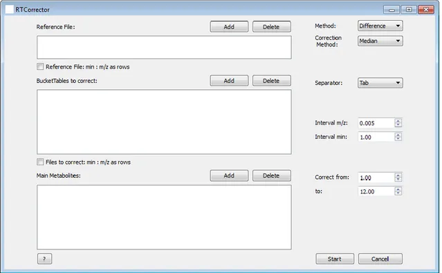
Accordingly, measurements must be performed with great care (see chapter 4.3.3). For severe (between-) batch effects we developed a correction strategy for retention time shifts to reduce missing values. Each batch is aligned sepa-

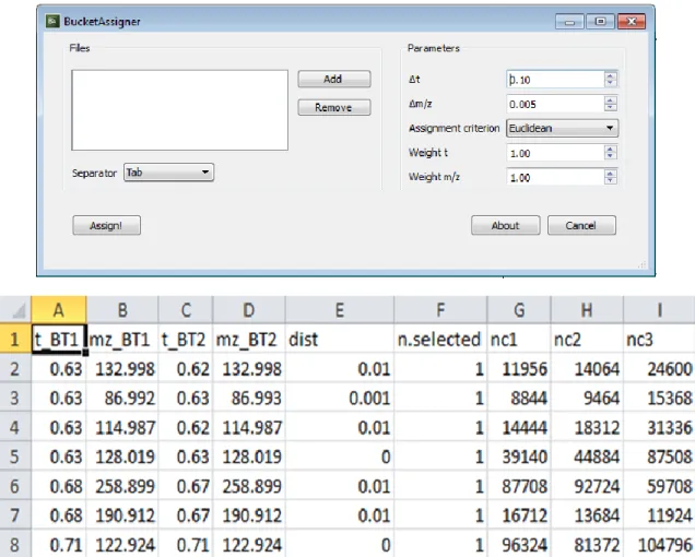
rately by the commercially available software which was in our case the Bruker Daltonics ProfileAnalysis software. Additionally, we developed a tool for correct- ing RT shifts according to one or more prominent compounds in the sample ma- trix. Differences in retention time for these house-keeping compounds are used to correct those of the remaining compounds (see chapter 5.4.3). Afterwards, with subsequent pairwise bucketing via an in-house written bucket assigner all the measured batches are combined (see chapter 5.4.4). The described proce- dure was applied in chapter 8. The Bucket assigner alone was also implement- ed in chapter 6. This procedure reduces missing values. Nevertheless, some missing values still remain in the data matrix because they are either true miss- ing values or the detected area is below the signal-to-noise threshold. Conse- quently, this requires imputation of the missing values prior to statistical analy- sis. Therefore, 1/10^th of the minimal detected area integral can be inserted. Al- ternatively, methods like missing completely at random or k-nearest neighbor imputation method (knn) can be utilized.^48,49 Moreover, prior to multivariate data analysis, it is necessary to reduce any variance in the data which is not biologi- cally induced. Strategies to avoid batch effects and technical variations in ad- vance are described in chapter 4.3.3. Different normalization methods were tested in this thesis to reduce any contribution from unwanted biases and exper- imental variance before and after the measurement of the urine samples (for details see chapter 6). However, normalization to the sum of all buckets can be utilized independent of the sample origin.

4.3.2 Data visualization and statistical analysis

Statistical analysis approaches applied for high throughput data like LC-MS da- ta are mainly adapted from earlier developed omic technologies.⁵⁰. Commonly, univariate or multivariate approaches are used in order to search for group sep- aration. Classical univariate analysis are the two-sided t-test or the analysis of variance (ANOVA) followed by a post-hoc test. Especially for large scale metabolomics where thousands of features are detected, it is important to cor- rect for multiple testing. Adjusting for multiple testing by controlling the false dis- covery rate according to Benjamini and Hochberg⁵¹ is an example for such a correction. Multivariate analysis methods use not only single discriminating me-

tabolites but also dependency structures to differentiate sample groups.⁵⁰ Most prominently utilized methods are principle component analysis (PCA), cluster analysis and classification methods like the random forest (RF) classifier. As a starting point for data analysis, the PCA is a very valuable tool to decrease complexity of large scale LC-MS data and to visualize differences between samples. Thereby, loading plots can help to identify discriminating metabolites.

Another popular method in metabolomics data analysis is the partial least squares discriminant analysis (PLS-DA).Instead of PCA, it is a supervised dis- criminant analysis method, which is dependent on class labels.⁵² In order to analyze high-throughput data in more detail, cluster analysis like hierarchical clustering is a valuable unsupervised method. For more details see chapter 5.5.1. The RF classifier is a supervised classification method based on decision trees. Therefore, the data set is split in two sets, training and test set.⁵³ Both are selected randomly applying resampling with replacement which is also known as bootstrapping. As the names intend, the training set is used to develop the decision tree and the test set is applied to calculate the classification accuracy.

53 According to the literature, the RF is a very accurate and robust classification method.⁵³ Support vector machine (SVMs) or regularized linear regression are alternative machine learning algorithms widely used in metabolomics data anal- ysis. These algorithms also use training sets to learn rules and form patterns, which then can be utilized to analyze new data.⁵⁴

4.3.3 Handling batch effects and technical variations

Batch effects, also called between-block effects, occur in large scale studies where samples are measured in several batches over an extended time period.

In order to prevent any kind of batch effects and technical variation, it is advisa- ble to consider the following experimental setup recommendations. Firstly, the samples should be measured in random order. Secondly, the instrument should be cleaned and calibrated before every measurement and the column should be equilibrated by injecting blanks and/or a standard before analyzing the sample sequence. Attention should also be paid to the eluent preparation and usage. It should be prepared exactly the same way every time. Blank samples must be measured repeatedly throughout the sequence in order to check for sample car- ry over and contaminations originating from the column. Moreover, quality con-

trol samples should be regularly interspersed throughout the measurement to investigate inter- and intra- batch effects. These QC samples can be used to check for batch effects including retention time shifts after the measurement.

4.4 Identification of metabolites by LC-MS analysis

As mentioned above, untargeted metabolomics is a retrospective analysis. In order to interpret the acquired data biologically, it is necessary to identify at least those metabolites that differentiate the biological groups the most. Howev- er, this is a very challenging and labor-intensive step especially for untargeted metabolomics of complex mixtures like urine, which contain exogenous as well as endogenous metabolites originating from individual diet, medication, life-style and environmental influences.⁵⁵ Moreover, the available databases (e.g. Human Metabolome Database (HMDB)⁵⁶, Metlin⁵⁷, Madison Metabolomics Consortium Database (MMCD)⁵⁸, MassBank⁵⁹, LIPID MAP⁶⁰) for metabolite identification from LC-MS data are limited in their content and a comprehensive database is missing.⁶¹ Therefore, it is almost impossible to identify all metabolites measured by an untargeted analysis. Sumner et al. introduced four levels of metabolite identification confidence.⁶² Metabolites with at least two orthogonal parameters e.g. accurate mass and RT identical to an authentic chemical standard meas- ured under the same analytical conditions are considered to be confidently iden- tified (level 1).^55,62 However, some metabolites and especially stereoisomers are very hard to distinguish even by comparison with an authentic chemical stand- ard.⁵⁵ This is due to almost identical RT and m/z values particularly in untarget- ed metabolomics where the analytical methods are needed to be very robust and fast. Therefore, these methods are not perfectly optimized.⁵⁵ In these cas- es, alternative analytical methods like NMR or GC-EI-MS need to be applied for a positive identification. In comparison to confidentially identified compounds, putatively identified compounds or classes (level 2 and level 3, respectively) are not confirmed by an authentic standard. Instead only one or two parameters are utilized to putatively identify metabolites by comparing them to data from librar- ies or other analytical properties from different laboratories.^55,62 In case of LC- MS measurements, such properties are accurately measured m/z values, RT or fragmentation patterns. Comparing the isotopic pattern to in-silico generated

pattern provides additional confidence. Level 4 metabolites are unknown com- pounds, which can nevertheless be differentiated by the chromatogram or mass spectra. Moreover, the relative quantification of level 4 metabolites is feasible.

However, a confident or putative identification is not possible. ^55,62

4.4.1 Identification workflow

The first step in the identification workflow is the calculation of the elemental formula of a certain accurate mass. This leads to a limited number of alterna- tives for the identification. However, for a reliable identification this number needs to be further reduced. Therefore, different filters and approaches are ap- plied.

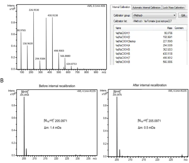
Firstly, the number of possible alternatives for the elemental composition can be limited by reducing the mass error. The more accurate the mass the lower is the number of possible elemental formulas.^63,64 Therefore, the detected masses should be internally recalibrated before calculating the elemental formulas. For this purpose, a sodium formate cluster injected via a six-port valve before every sample run can be utilized. The sodium formate cluster contains representative masses across the required mass range (see Fig.4.2 A). After measurement the mass spectrum of the sodium formate cluster is used to recalibrate the mass scale, improving the mass accuracy of the measured compounds (see Fig.4.2.

B).

Figure 4.2: A sodium formate cluster is applied for external and internal mass calibration of HPLC-ESI-qTOF-MS measurements. (A) The mass spectrum of the sodium formate cluster, which is infused at the beginning of each sample analysis, is depicted on the left. The corre- sponding mass list of the recalibration method is shown on the right. (B) The improvement of the mass accuracy after recalibration is illustrated for tryptophan exemplarily.

Secondly, potential elements and adducts should be initially selected before calculating the elemental formula of an accurate mass in order to avoid false alternatives from including all elements from the periodic table.⁶⁴ Of course, cer- tain knowledge about the source of the unknown is necessary.

Furthermore, tools like SmartFormula from Bruker Daltonics (Bremen, Germa- ny) calculate the elemental composition from accurate masses by considering the rings-plus-double-bonds equivalent (RDBE), the nitrogen rule, the isotopic pattern as well as heuristic and chemical rules as introduced by Kind and Fiehn in 2007.⁶⁵ Consequently, these tools further constrain the composition of ele-

mental formulas fitting an accurate mass. The RDBE is calculated by the follow- ing formula:

𝑅𝐷𝐵𝐸 = 𝑁_𝐶+ 𝑁_𝑆𝑖− 1

2 (𝑁_𝐻+ 𝑁_𝐹+ 𝑁_𝐶𝑙 + 𝑁_𝐵𝑟+ 𝑁_𝐼) + 1

2 (𝑁_𝑁+ 𝑁_𝑃) + 1 Here, N stands for the amount of atoms of the corresponding element.⁶⁵ The nitrogen rule states that an odd nominal molecular mass also implies an odd number of nitrogen atoms.⁶⁵

In 2006, Kind and Fiehn showed the advantage of using isotopic abundance pattern as an additional filter for calculating elemental formulas.⁶³ They com- pared a MS with 3 ppm mass accuracy applying the isotopic pattern filter (2%

error) to a MS with less than 1 ppm mass accuracy omitting the isotopic pattern as a filter. They demonstrated that high mass accuracy alone is insufficient in order to reduce the number of possible elemental formulas especially for candi- dates with complex elemental compositions.⁶³ Even a hypothetical mass spec- trometer with 0.1 ppm mass accuracy was outperformed by the additional iso- topic pattern filter.⁶³ Therefore, the implementation of filters using the isotopic abundance pattern, removes most of the falsely assigned elemental formulas.⁶³ The isotopic pattern fit is evaluated by the calculation of the mSigma value in the SmartFormula tool from Bruker Daltonics. In the case of a perfect match the mSigma value is 0, whereas a value of 1000 means no match.

After limiting the number of possible molecular formulas, whereby preferably only one elemental formula is left, available data bases like HMDB⁵⁶, Metlin⁵⁷ or ChEBI (Chemical Entities of Biological Interest)⁶⁶ are searched for the chemical structure. However, the knowledge of the mass spectrometrist about the sam- ples under investigation is an essential and mandatory requirement for the cor- rect assignment of a chemical structure. As mentioned above, another aspect to positively identify an unknown signal is the corresponding fragmentation pat- tern. Holcapek et al. summarized the fragmentation behaviors of individual func- tional groups in 2010.⁶⁷ Hence, MS/MS experiments can increase the knowledge on the identification of the signal under investigation.⁶⁴

Finally, the comparison to an authentic chemical standard is the last step in the identification workflow. The measured RT, isotopic pattern and fragmentation pattern from the standard should be compared to the unknown. The unambigu-

ous identification of an unknown requires the additional measurement with an independent analytical method such as NMR.

4.4.2 Concrete examples for LC-MS based identification

Here, the LC-MS based identification workflow and its significant role in metabo- lomics is exemplarily shown.

In the following, the identification procedures are partly adapted from Dettmer et al. 2013 and Zacharias et al. 2015, respectively.^30,68

In Dettmer et al. 2013, metabolic footprinting of the cell culture supernatants of 20 human cancer cell lines and 4 primary cell cultures was conducted by means of high-resolution LC-QTOF-MS.⁶⁸ Statistical analysis resulted in 391 differential features after correction for multiple testing. The 49 most significant features and five additional features were then identified according to Fig. 4.3. Here, ex- emplarily the identification workflow of arginine, which was the most discriminat- ing feature, is shown. Furthermore, MS/MS experiments were performed and the MS/MS spectra were compared to the METLIN library. The identification of the most significant features showed interesting insights into cancer metabo- lism. It revealed extracellular arginine and nicotinamide as major discriminants between normal and neoplastic hepatocytes. Further, the observed significant differences in the assimilation of di- and tripeptides appeared to underscore the increased bioenergetic and biosynthetic demands of many cancers.⁶⁸ These findings emphasize the importance of metabolite identification via high resolu- tion LC-MS.

Figure 4.3: Exemplary workflow for the identification of unknown LC-ESI-qTOF-MS features that discriminate between different cell types. The Bruker tools SmartFormula and Compound Crawler were employed for the identification. The tentative identification of arginine was con- firmed with an authentic chemical standard.

In the study by Zaccharias et al. (2015), LC-QTOF-MS contributed to the identi- fication of the most significant metabolite for the prognostication of acute kidney injury (AKI) patients after cardiac surgery with cardiopulmonary bypass.³⁰ A well resolved NMR signal was found in plasma samples that distinguished patients, who developed AKI, from those that did not experience AKI. However, it was not possible to identify this signal by database searches or by 2D 1H TOCSY,1H−13C HSQC, and 1H−13C HMBC spectra, respectively. Therefore, 5 AKI and 5 non-AKI plasma samples were investigated by LC-QTOF-MS. After

correction for multiple testing, 11 significant features remained. Identification was performed as shown exemplarily in Fig. 4.3 and standards were purchased for the most promising hits. MS/MS experiments were performed on both the standards and the plasma specimens for additional verification. Among the most discriminating features, the propofol metabolites propofol glucuronide and 4-hydroxy-propofol-1-OH-D-glucuronide were positively identified. 1D 1H NMR reference spectra were acquired on these compounds and unambiguously veri- fied the assignment of the NMR signal.³⁰

5. Experimental section

5.1 Materials

Deionized water (PureLab Plus system, ELGA LabWater, Celle, Germany) cre- atinine-D3 (C/D/N Isotopes, Pointe-Claire, Canada), HPLC-grade acetonitrile (ACN) were purchased from VWR International (Vienna, Austria). Formic acid, uric acid, 1-methyluric acid, phenylacetic acid, phenyllactic acid, 3-(4- hydroxyphenyl)propionic acid, indoxyl-sulfate, creatine, creatinine, hippuric acid, guanidinoacetic acid, hypoxanthine, methylxanthine, kynurenic acid, DL- kynurenine, DL-tryptophan, xanthurenic acid, 3-hydroxyanthranillic acid, 3- indolacetic acid, 3,4-dihydroxy-L-phenylalanine, indole, DL-3-indolelactic acid, 3-indolepropionic acid, indole-3-carboxaldehyde, 3-indolepyruvic acid, trypta- mine, tryptophol, nicotinic acid, melatonin, 3-hydroxy-DL-kynurenine, 5- hydroxyindole-3-acetic acid, 1,7-dimethylxanthine, serotonine hydrochloride, xanthine, nicotinamide, quinolinic acid, anthranilic acid, ammonium hydroxide and sodium hydroxide were purchased from Sigma-Aldrich/Fluka (Taufkirchen, Germany). Isopropanol (VWR), propofol (Toronto Research Chemicals, Toron- to, Ontario, Canada).

5.2 Sample preparation

If not indicated otherwise, all urine specimens were diluted 1:4 with deionized water either directly in 1.5-mL glass vials with 0.2-mL micro-inserts (Machery- Nagel, Düren, Germany) or in micro-reaction tubes and subsequently trans- ferred into the glass vials.

5.3 Instrumentation

5.3.1 HPLC-ESI-TOFMS

A Thermo Scientific Dionex Ultimate 3000 UHPLC system (Idstein, Germany) consisting of the HPG3400 RS pumping system, the TCC-3000 RS column ov-

en and the WPS3000TFC autosampler was coupled to a Maxis Impact QTOF- MS (Bruker Daltonics, Bremen, Germany) through an ESI source. A KinetexTM C18 column (100 mm x 2.1 mm id x 2.6 µm C18 1000, Phenomenex, Aschaf- fenburg, Germany) with a SecurityGuard ULTRA C18 cartridge (Phenomenex) as a pre-column was applied to separation in chapter 6 and to the fingerprinting measurements in chapter 8. The column oven temperature was set at 35°C.

The chromatographic separation was accomplished by applying 0.1% (v/v) for- mic acid in water as mobile phase A and 0.1% (v/v) formic acid in ACN as mo- bile phase B at a flow rate of 0.3 mL/min. Elution was accomplished by the fol- lowing ACN gradient unless stated otherwise in the text: 0-40% in 10 min, 40- 100% in 2 min, 100% for 5 min, back to 0% in 0.1 min, 5 min equilibration. An injection volume of 5 µL was used unless otherwise noted in the text. The ESI source was operated in positive mode applying the following settings for the source and the mass spectrometer: drying gas: nitrogen with a temperature of 220 °C and a flow rate of 10 L/min; pressure of the nebulizer gas (nitrogen): 2.6 bar; end plate offset: 500 V; capillary voltage: 4500 V; mass range: 50-1000 m/z; acquisition rate: 5 spectra/s. Before the measurements, an external cali- bration of the mass spectrometer was implemented using sodium formate clus- ters (10 mM). Therefore, 12.5 mL of water, 12.5 mL of isopropanol, 50 µL of formic acid (conc.) and 250 µL of 1M NaOH were mixed. Additionally, each run was started with an injection of the sodium formate solution by means of a six- port valve for internal recalibration (see section 4.4.1).

5.3.2 HPLC-ESI-QqQMS

A 1200 SL HPLC (Agilent, Böblingen,Germany) was coupled to an Applied Bio- systems 4000 QTRAP mass spectrometer (Sciex, Darmstadt, Germany) via a TurboV ESI source operating either in positive or negative ionization mode. For separation a Waters (Eschborn, Germany) Atlantis T3 column (2.1 x 150 mm i.d., 3 µm) at 25°C was used, applying 0.1% (v/v) formic acid in water as mobile phase A and 0.1% (v/v) formic acid in ACN as mobile phase B at a flow rate of 0.4 mL/min. The elution of the analytes detected in positive and negative mode was achieved by the following ACN gradient: 0% to 50% in 1 min, 50% for 5 min, back to 0% in 0.1 min, 4 min equilibration. This gradient is equivalent to the

gradient used by Zhu et al. (2011).⁶⁹ An injection volume of 10 µL was utilized.

The MS parameters for each metabolite were optimized by direct infusion via a syringe pump (Harvard Apparatus, Holliston, MA, USA).

5.3.3 Miscellaneous

In the course of this doctoral research work the following other lab equipment was utilized: a heater with two heating blocks (Haep Labor Consult, Bovenden, Germany), a vortexer (lab dancer, IKA-Werke GmbH, Staufen, Germany) and a model himac CT15RE centrifuge from Hitachi (Düsseldorf, Germany).

5.4 Data analysis

5.4.1 Software

DataAnalysis version 4.1 (Bruker Daltonics) was utilized for manual examination and processing of the HPLC-TOF-MS chromatograms and mass spectra, com- pound extraction, internal recalibration of the mass spectra, and calculation of accurate masses, elemental formulas and mSigma values as well as for feature extraction from the chromatograms by the Find Molecular Feature (FMF) algo- rithm. ProfileAnalysis version 2.2 (64-bit) (Bruker Daltonics) was employed for feature alignment. Bucket tables were then exported and further analyzed with the R package version 3.1.1⁷⁰ and Excel (Microsoft Corporation, Redmond, WA). Bland Altman plots as well as basic statistics e.g. the calculation of rela- tive standard deviations (RSDs), paired student’s t test, spearman rank correla- tion coefficients (SCC) as well as Pearson correlation coefficients was per- formed with Excel. R was used to generate box plots and Venn diagrams as well as to perform principle component analysis (PCA), hierarchical cluster analysis by using Pvclust⁷¹, Shapiro-Wilk test and to calculate false discovery rates (FDRs) according to Benjamini and Hochberg⁵¹ using MULTTEST⁷². MassLynx (Waters, Eschborn, Germany) was used for manual reintegration and quantification of specific analytes in chapters 6 and 8. The Analyst (Applied Bio- systems/MDS Sciex, Darmstadt, Germany) software was used for calculating