Testing for Stationarity in a Cointegrated System

IHS Economics Series Working Paper 117

July 2002

Testing for Stationarity in a Cointegrated System

Robert M. Kunst

Impressum Author(s):

Robert M. Kunst Title:

Testing for Stationarity in a Cointegrated System ISSN: Unspecified

2002 Institut für Höhere Studien - Institute for Advanced Studies (IHS) Josefstädter Straße 39, A-1080 Wien

E-Mail: o ce@ihs.ac.atffi Web: ww w .ihs.ac. a t

All IHS Working Papers are available online: http://irihs. ihs. ac.at/view/ihs_series/

Testing for Stationarity in a Cointegrated System

Robert M. Kunst

117

Reihe Ökonomie

Economics Series

117 Reihe Ökonomie Economics Series

Testing for Stationarity in a Cointegrated System

Robert M. Kunst

July 2002

Contact:

Robert M. Kunst University of Vienna and

Institute for Advanced Studies Department of Economics and Finance Stumpergasse 56, A-1060 Vienna, Austria (: +43/1/599 91-255

email: robert.kunst@ihs.ac.at

Founded in 1963 by two prominent Austrians living in exile – the sociologist Paul F. Lazarsfeld and the economist Oskar Morgenstern – with the financial support from the Ford Foundation, the Austrian Federal Ministry of Education and the City of Vienna, the Institute for Advanced Studies (IHS) is the first institution for postgraduate education and research in economics and the social sciences in Austria.

The Economics Series presents research done at the Department of Economics and Finance and aims to share “work in progress” in a timely way before formal publication. As usual, authors bear full responsibility for the content of their contributions.

Das Institut für Höhere Studien (IHS) wurde im Jahr 1963 von zwei prominenten Exilösterreichern – dem Soziologen Paul F. Lazarsfeld und dem Ökonomen Oskar Morgenstern – mit Hilfe der Ford- Stiftung, des Österreichischen Bundesministeriums für Unterricht und der Stadt Wien gegründet und ist somit die erste nachuniversitäre Lehr- und Forschungsstätte für die Sozial- und Wirtschafts - wissenschaften in Österreich. Die Reihe Ökonomie bietet Einblick in die Forschungsarbeit der Abteilung für Ökonomie und Finanzwirtschaft und verfolgt das Ziel, abteilungsinterne Diskussionsbeiträge einer breiteren fachinternen Öffentlichkeit zugänglich zu machen. Die inhaltliche

Abstract

In systems of variables with a specified or already identified cointegrating rank, stationarity of component variates can be tested by a simple restriction test. The implied decision is often in conflict with the outcome of unit root tests on the same variables. Using a framework of Bayes testing and decision contours, this paper searches for a solution to such conflict situations in sample sizes of empirical relevance. It evolves from the decision contour evaluations that the best test to be used jointly with a restriction test on self-cointegration is a modified version of the Dickey-Fuller test that accounts for the other system variables, whereas strictly univariate unit-root tests do not help much in the decision of interest.

Keywords

Bayes Test, unit roots, cointegration, decision contours

JEL Classifications

C11, C12, C15, C32

Contents

1 Introduction 1

2 Testing for unit roots in cointegrated systems 3

2.1 A standard test for a unit root...3

2.2 Traditional non-standard tests for unit roots...5

2.3 Multivariate augmentation of the Dickey-Fuller test...6

2.4 The geometry of the problem...7

3 A comparison of tests 8

3.2 Imposing stationarity as a cointegration restriction in an AR(1) model... 10

3.3 Imposing stationarity as a cointegration restriction in an AR(2) model... 12

3.4 Decision boundaries... 14

4 Results of the simulations 16

5 Summary and conclusion 20

References 21

Figures 23

1 Introduction

The procedure designed by Johansen for the estimation of the cointegrat- ing rank and of the cointegrating vectors in vector autoregressive systems has enjoyed tremendous popularity among researchers in economic applica- tions. Usually, the procedure is conducted in several sequential steps. First, univariate unit-root tests classify the variables of interest according to their degree of integration. Variables integrated of order zero or one are kept while higher-order integrated variables are eliminated or di¤erenced. Then, the cointegrating rank is determined. Last, linear restriction tests are ap- plied that check whether pre-speci…ed vectors of interest are contained in the cointegrating space. In other words, the basis of the cointegrating space is rotated in order to become interpretable in economic terms.

Unit vectors may be contained in the cointegrating space. Whenever a unit vector cointegrates, the corresponding component variable is stationary.

Practitioners often report that the decision resulting from the restriction testing step of Johansen’s procedure disagrees with the decision of the pre- liminary unit-root tests. A speci…c variable may be classi…ed as stationary ac- cording to the preliminary univariate unit-root test and as non-cointegrating according to the restriction test, and vice versa. The natural question is then how to combine these contradictory pieces of evidence to reach a statistically well-based classi…cation of these problematic variables.

We note that many researchers tend to avoid including stationary vari- ables in the Johansen framework, although the procedure has been designed to incorporate cases with integration order zero as well. The statement that all individual components must be integrated of order one is erroneous, al- though it can be found in some sources, including software descriptions. In the spirit of the procedure, stationary components imply cointegrating unit vectors, in other words the stationary variable is cointegrating with itself.

The hypothesis that a speci…c unit vector is contained in the cointegration space can be subjected to a restriction test after determination of the rank and estimation of the full system (‘post-testing’). In contrast with most pre- liminary unit-root tests, stationarity of the component is the null hypothesis of these restriction tests and …rst-order integration is the alternative. The distribution of the corresponding test statistic is chi-square and not any of the non-standard mixture distributions that are known from the unit-root testing literature (see also Tanaka, 1996).

In related work, Rahbek and Mosconi (1999) use a slightly di¤erent

model frame and view cointegration as conditional on stationary variables that may develop cointegration among their cumulated sums. For the full system of conditioned integrated and conditioning stationary variables, a vector autoregressive representation does not exist. In contrast, we assume the existence of a multivariate autoregressive representation for the whole vector of variables, in line with the original model that was analyzed by Johansen (1995).

This paper attempts to answer some of the questions that are implied by the outlined procedure. Firstly, how can a unit-root test exist with standard critical values, if the construction of non-standard critical points was one of the main tasks of the early literature on unit-root tests. Secondly, how should one act in cases of con‡ict? Cases of con‡ict arise from changes in the identi…ed integration order between the pre-testing and the post-testing phase. A variable may be classi…ed as stationary in the pre-testing stage but its unit vector is rejected as a cointegrating vector in post-testing. Conversely, a variable may be classi…ed as …rst-order integrated in pre-testing but its unit vector is accepted as cointegrating in post-testing. In the former case, we will ignore the potential con‡ict situation where a cointegrating rank of zero has been found in the main testing stage, as it appears altogether unlikely and may point to a more general speci…cation failure.

In order to avoid distracting attention from the main focus, important side issues will be ignored in this paper, such as the possible appearance of seasonal unit roots, the complex restriction test for second-order integration within the framework of the multivariate Johansen procedure, or the correct speci…cation of the deterministic features of the system.

The outline of this paper is as follows. Section 2 describes three hypothesis

tests that are more or less commonly used in discriminating stationary and

integrated variables. Section 3 introduces the semi-Bayesian method that is

suggested for evaluating combinations of any two of these tests. The results

of an application of this suggested method are presented and commented in

Section 4. Section 5 concludes.

2 Testing for unit roots in cointegrated sys- tems

2.1 A standard test for a unit root

Suppose the vector variable X

has n components that are individually either I(0) or I(1), and obeys a vector autoregression of order p

©(B )X

= ¹ + "

with "

an ideally Gaussian white noise. Then, the system can be transformed into its error-correction representation

¦(B)¢X

= ¹ + ®¯

X

+ "

with n £ r–matrices ®; ¯ of full rank that are uniquely determined up to a non-singular matrix factor of dimension r £ r. r denotes the cointegrating rank, ¯ is the matrix with cointegrating column vectors, and ® is the so-called loading matrix. ¦(z) is a polynomial of order p ¡ 1.

In line with many applications of the Johansen procedure, only a con- stant ¹ is allowed as the deterministic part of this model, which is a debatable choice. It is at odds with the common usage of trend regressors in univari- ate unit-root tests, which are included for the sake of similarity properties at the expense of test power, but it is in line with the usual interpretation of error correction. A linear combination of non-stationary variables that is trend-stationary does not correspond to this concept.

If X contains an I(0) component X

, say, the unit n–vector with 1 at its j th entry and 0 otherwise is contained in the column space of ¯. This implies that r ¸ n

if n

denotes the number of stationary components. If r = n

, there is no non-trivial cointegration in the system, as all cointegrating vectors are unit vectors or linear combinations thereof. If r = n = n

, the whole system is stationary. Without restricting generality, assume that the variable in question is the …rst one X

such that the critical cointegrating vector is e

= (1; 0; : : : ; 0)

. Then, the hypothesis would be

¯ = (e

; ') ; (1)

where ' is an n £ (r ¡ 1)–matrix. Because ¯ is identi…ed only up to an

r £ r transformation matrix, identifying its …rst column with the proposed

basis vector implies no restriction of generality. For this problem, Johansen (1995, p. 108) shows that ¯ is estimated by a sequence of conditioning opera- tions. When e

is the only cointegrating vector, the solution is extremely sim- ple, as then the system reduces to ¦(B )¢X

= ¹+ ®X

+"

, a multivariate regression problem. The likelihood-ratio statistic T f ln(1 ¡ ¸

) ¡ ln(1 ¡ ½) g of this restricted solution versus the solution for unrestricted r–dimensional ¯ is distributed as chi-square with n ¡ r degrees of freedom. Here, ¸

denotes the largest eigenvalue of the unrestricted problem and ½ is the conditional multiple correlation of X

and ¢X

. This ½ can be obtained from …rst re- gressing both sides on a constant and on lagged di¤erences and keeping the residuals. Then, the possibly non-stationary residual from the ‘purged’ X

is regressed on the similarly …ltered ¢X

. The R

of this second regression is the required ½.

Under the null hypothesis of this test, the component variable is station- ary, as the corresponding unit vector cointegrates. However, the alternative is not the usual general hypothesis of …rst-order integration. Rather, the presence of r cointegrating relationships or of n ¡ r unit roots in the system is maintained. Therefore, the test is not a valid unit-root test for general pur- poses, although it is a valid check on univariate unit roots conditional on an already speci…ed cointegrating rank. Note that, in the system, the same num- ber of unit roots is present under the null and under the alternative, which explains the validity of the standard distribution for the likelihood-ratio test.

Some of these issues have been considered by Horvath and Watson (1995) who analyze the general case of testing for given cointegrating vectors, which includes unit vectors as a special case. Because they set up the problem in such a way that the given vector does not cointegrate under the alternative, they obtain non-standard distributions, contrary to the original Johansen idea. The use of multivariate VAR analysis for assessing the stationarity of individual components is mentioned by Johansen and Juselius (1992) who assume the cointegrating rank as having been pre-tested and therefore

…xed. Most applications proceed (correctly) by …rst identifying the rank and

then testing for special vectors, hence the original approach is in focus here.

2.2 Traditional non-standard tests for unit roots

For a scalar variable x

, the most popular test for unit roots is based on the t–statistic on ¯ in the regression

¢x

= a + bt + ¯x

+ X

j=1

¼

¢x

+ "

: (2) The null hypothesis is one unit root in the autoregressive operator for x

, i.e., '(1) = 0 for ' (z) = (1 ¡ P

j=1

¼

z

)(1 ¡ z) ¡ ¯z or, equivalently, ¯ = 0. The alternative is that '(z) has stable roots only. Although this test, whose idea is due to Dickey and Fuller (1979), has been criticized in the literature (for a critical review, see Maddala and Kim, 1998), its apparent simplicity is one of its greatest virtues. Also note that it exactly corresponds to an univariate version of the Johansen test for cointegration. Hence, one of the key arguments against the DF test, i.e., doubts on the autoregressive nature of the generating mechanism, is misplaced in the setting of the Johansen procedure, which assumes an autoregression for the system variable X

.

Like the multivariate Johansen procedure, the univariate Dickey-Fuller test can be used with several combinations of deterministic terms. Because the test is often used to discriminate drifting integrated from trend-stationary variables, it makes sense to use the test as in (2), though the set-up of hy- potheses is then non-standard, as b is implicitly restricted under the null.

In the model that is investigated here, i.e., the multivariate autoregression with a constant, trend-stationary variables can only appear in paradox cases and are therefore best excluded. Hence the speci…cation without the trend regressor deserves consideration.

For the pre-test stage in the Johansen procedure, unit-root tests are com-

monly applied with the aim of classifying the variables into one out of three

classes: I(0), I(1), and I(2) variables. According to what is sometimes known

as the Pantula principle (after Pantula, 1989), a two-stage sequence of

Dickey-Fuller tests starts with testing the I(2) null hypothesis against an

I(0) [ I(1) alternative ‘I(0/1)’, then in case of …rst-stage rejection an I(1) null

is tested against an I(0) alternative. It was outlined above that the second

test in the sequence is potentially unnecessary, as I(0) variables are treated

correctly in the comprehensive multivariate model. The …rst stage, however,

serves to eliminate objects outside the focus of the analysis. Unless the re-

searcher decides to proceed with the …rst di¤erence of the original variables,

which has been suggested for certain price series, the …rst Dickey-Fuller test is really a speci…cation test and is comparable to tests for breaks, non-normality etc. This speci…cation test is not in focus here.

2.3 Multivariate augmentation of the Dickey-Fuller test

It may be argued that a comparison of the Dickey-Fuller test and the post- test of Johansen is not appropriate, as the latter incorporates multivariate information whereas the former is strictly univariate. Notwithstanding the swap of null and alternative hypotheses, the multivariate test has the advan- tage of processing more ‘information’, which may improve its discriminatory power. Multivariate information can easily be incorporated into the Dickey- Fuller test. For example, assuming a second variable y

to be I(0/1), the t–statistic on ¯ in the regression

¢x

= a + bt + ¯x

+

p¡1

X

j=1

¼

¢x

+

p¡1

X

j=1

~

¼

¢y

+ "

(3) will have similar asymptotic properties to the original Dickey-Fuller test.

Using certain assumptions, Hansen (1995) shows that the null distribution of t

is a mixture of Dickey-Fuller and standard distributions. Although Hansen develops his results in a univariate regression framework conditional on ¢y

, (3) can also be viewed as a component in a vector autoregression. For demonstration, assume a …rst-order vector autoregression for the variables (¢x

; ¢y

) augmented by a lag of x

, i.e.,

¢x

= ®

x

+ ¼

¢x

+ ¼

¢y

+ "

¢y

= ®

x

+ ¼

¢x

+ ¼

¢y

+ "

:

This is the general form for a VAR on (x

; ¢y

) with mixed lag orders of two

and one for the variables. This is also an error-correction representation for

a second-order VAR on (x

; y

) with the potential cointegrating vector (1; 0)

assumed as known. For the parameter value (®

; ®

) = (0; 0), both variables

are I(1) and there is no cointegration. For ®

6 = 0 and arbitrary ®

, x

is

self-cointegrating and stationary while y

is I(1). The case ®

= 0 and ®

6 = 0

is not possible, as it violates the assumption that both variables are I(0) or

I(1). Honoring Hansen, the t–test for ®

= 0 (or ®

= 0) will be called the

CADF (covariate-augmented Dickey-Fuller) test in the following.

Any stationary augmentation is possible, although cointegrating condi- tioning variables will still be ignored. An augmentation by ‘level’ I(0/1) variables is not possible, as these may be cointegrated with the x

regres- sor and may therefore impair the evidence on stationarity in x

.

2.4 The geometry of the problem

In traditional Neyman-Pearson testing, usually the lower-dimensional hy- pothesis is chosen as the ‘null’ hypothesis and the higher-dimensional one as the ‘alternative’. Occurrences of dimension change between null and alter- native in comparable tests may draw special attention. In many apparent events of dimension change, such as the pair of the Dickey-Fuller and the Saikkonen-Luukkonen tests that was analyzed by Hatanaka (1995), null and alternative are embedded in parametric modeling frames that only par- tially overlap. For example, the unit-root hypothesis is ‘small’ within …rst- order autoregressions that do not include over-di¤erenced time series, and is large within …rst-order moving-average models for the di¤erenced series that do not include autoregressions excepting white noise. In these problems, the

‘true’ null and alternative hypotheses of interest to the researcher are insuf-

…ciently matched by the limited structures of both parametric models. The present case is inherently di¤erent.

Dickey-Fuller tests, or comparable unit-root test procedures for a single series in a bivariate vector autoregressive frame, can best be seen as con- densing the classi…cation problem for the overall number of unit roots in the system. This system might have no, one, two, or more unit roots, though for the needs outlined here, it is preferable to exclude the cases of more than two unit roots, of two or more unit roots within a single direction, and of explosive roots. Let us denote the three basic hypotheses by £

, £

, and

£

. The null hypothesis of the DF test then consists of £

and a part of £

, while the alternative comprises £

and the remainder of £

. £

is a set of lower dimension within £

[ £

, while £

[ £

is again of lower dimension within the maintained hypothesis or general frame £

[ £

[ £

. One may envisage a point (£

) on a curve (£

[ £

) on a plane (£

[ £

[ £

). The point and a part of the curve constitute the null and the remaining plane constitutes the alternative of the DF test.

In the Johansen test, interest focuses on the curve. The point £

, the

case of no cointegration, has been excluded in the preliminary step. The

punctured curve is isomorphic to a half-open interval of angular frequencies,

such as [0; ¼), which represent the direction of the cointegrating vectors in the (x

; x

)–plane. For the points 0 and ¼=2, one of the two series is stationary by self-cointegration, while for all other points a non-trivial linear combination of the two variables is needed to achieve stationarity. Then, for example, the sliced background plane £

and the end point of this interval constitute the null hypothesis, while the open interval (0; ¼) constitutes the alternative.

Identifying the cointegrating rank as 1 …nally excludes the sliced background plane, and the researcher is left with the traditional testing problem with a point null and an interval alternative.

This analysis implies that, contrary to the more involved problem investi- gated by Hatanaka (1995), no real change of the reference frame has taken place. Rather, the exchange of null and alternative is caused by restricting attention to a part of the original parameter space.

3 A comparison of tests

The debate on the correct way of assessing the merits of a joint application of hypothesis tests with exchanged null and alternative hypotheses remains unresolved in statistics. So-called con…rmatory analysis (see Charemza and Syczewska, 1998) is shunned in the literature (see Maddala and Kim, 1998). This technique, although of interest in its own right, is still

‘local’ in the sense that it evaluates test power and size at speci…ed points of the parameter space. This may imply the verdict that the prescription of the joint picture is of little help to the practitioner, as it is exactly this point of the parameter space that is unknown, or testing would otherwise not be necessary. By contrast, traditional Bayes testing is ‘global’ in the sense that the points of the parameter space are weighted by a prior distribution.

Critics of Bayes testing point out the sensitivity of the global decision to the choice of such prior distributions, while practitioners are often reluctant to conduct the lengthy computation that is involved in the calculation of posterior odds by way of numerical integration.

In previous work (see Kunst and Reutter, 2002), a compromise be- tween frequentist (local) and Bayesian (global) evaluation principles was sug- gested that was inspired by the work of Hatanaka (1995). It was attempted to standardize the prior distributions for both hypotheses in such a way that each hypothesis is given an a priori weight of 0.5. In this setting, the labels

‘null’ and ‘alternative’ are certainly incorrect and will be replaced by hypoth-

esis A and B in the following. The hypotheses correspond to parts of the parameter space with possibly identical dimensionality, and the frequentist interpretation swaps across tests. The basic problem should rather be seen as involving a parameter space £ that is partitioned into £

and £

and a decision that is searched for regarding whether the unknown µ is in £

or in £

. Unfortunately, prior distributions over these parameter spaces have also to be de…ned, and such priors necessarily involve some arbitrariness.

However, once such a prior speci…cation is accepted, further proceeding is very simple. Finite trajectories of processes can be generated from a vector of normal random numbers, conditional on a parameter µ drawn from the prior over £. From each trajectory, statistics and, for example, their nominal p–values can be calculated. A bivariate (0; 1) £ (0; 1)–diagram can be drawn from these p–values and can be split into small grid bins. Each bin contains a large quantity of similar pairs of p–values that correspond to statistics that, in turn, stem from a variety of trajectories. If most trajectories stem from

£

, then hypothesis A is seen to dominate the bin. The researcher, who just observes the statistics or p–values but does not know µ, will then decide in favor of hypothesis A. Otherwise she will decide for B. This technique can be applied to various joint testing problems and it will also be applied here.

The di¤erence between the ‘local’ and ‘global’ approach can also be seen as follows. The local (or traditional) approach conditions the analysis and all simulations on the generated model, i.e., on the true parameters. This is helpful for studying theoretical properties but does not provide much help to the practitioner. The global approach conditions all analysis and simulations on the observed statistics. The simulation design is varied over virtually ‘all’

possible data-generating processes. A given value of the observed statistic may have been produced by any value of the parameter space but it may be connected more frequently to one of the two subspaces (hypotheses). This then helps the practitioner who also observes a pair of test statistics and knows that the more probable hypothesis is the preferred decision.

3.1 Prior distributions within the frame

Current statistics operates under the double assumption of, …rstly, a true data

generation mechanism and, secondly, a researcher whose task it is to decode

this true data generation mechanism from a …nite amount of data. In time

series, data come in the form of trajectories of …nite length. Typically, the

available data even form a single trajectory which may have been generated

by any member of an assumed a priori model frame and may also have been generated from some non-member. Given this situation, any evidence on misspeci…cation—meaning that the data have been generated by a non- member—is unlikely to be trustworthy.

As an alternative aaproach, we suggest proceeding in the following way.

Firstly, the researcher assumes a frame, i.e., a parameterized model class that is large enough to make it a priori conceivable that the data have been generated by one of its members and at the same time small enough to keep the estimation problem tractable. Secondly, …nd the parameter value that has most likely generated the given data, conditional on restricting one’s attention to the frame. The implied parameter is usually known as a quasi- maximum likelihood estimate ^ µ 2 £. This solves the problem of estimation.

In order to determine whether the observed data are more likely to have been generated by £

or by £

, it does not su¢ce to look whether ^ µ 2 £

or ^ µ 2 £

, particularly if one of the two hypothesis sets is lower-dimensional.

In many cases, such a decision is inspired by a high a priori probability of µ being a member of the lower-dimensional part. We express this a priori probability by assigning a weight of 0.5 to either hypothesis. In the cur- rent problem, the model frame consists of vector autoregressions with given cointegrating dimension.

The elicitation will now be highlighted on the basis of an assumed cointe- grating rank of one. The cases of …rst- and second-order autoregression will be treated. Generalizations are then straightforward.

3.2 Imposing stationarity as a cointegration restriction in an AR(1) model

The …rst-order autoregressive model with a cointegrating rank of one can be written as

¢X

= ¹ + ®¯

X

+ "

with the n–vectors ¹; ®; ¯. If the system is to be stable apart from the integrating directions, the eigenvalues of ¦ = I+®¯

are in the range [ ¡ 1; 1].

More particularly, n ¡ 1 eigenvalues will be 1 and one eigenvalue is in the open interval ( ¡ 1; 1). The model has 3n free parameters, as f ®; ¯ g is of dimension 2n ¡ 1 due to arbitrary scaling.

It follows that a simple and good a priori distribution over £ = f (®

; ¯

;

¹

; ¾

)

: n ¡ 1 roots are 1, 1 root is stable g assumes the following speci…ca-

tions:

¦ = Z

· ¸ 0

0

I

¸ Z

with

Z

= 1; j = 1; : : : ; n;

Z

» N(0; ¾

); j 6 = k;

¹ » N(0; ¾

I

)

¸ » U ( ¡ 1; 1)

The variance parameters ¾

; ¾

; ¾

cannot be given improper prior distribu- tions in the Bayesian style, as the model will be simulated and one cannot draw from an improper distribution. Because the test decision is seen to be invariant in ¾

anyway, ¾

´ 1 is set and the possible reaction to mod- i…cations of the hyperparameters ¾

and ¾

is then studied. In the basic experiments to be reported in Section 3.2, we set ¾

= 0 and ¾

= ¾

. In one case, variations of relative variance will be studied. The implied distribution for the matrix ¦ is a special case of the Jordan distribution family introduced in Kunst (1995). The de…nition of £ excludes some lower-dimensional man- ifolds from R £ S

£S

£ R

£ R

, such as the case of n = 2; ® = (1; 0)

;

¯ = (0; 1)

, which would give rise to second-order integration. S

is the surface of the n–dimensional unit sphere and has dimension n ¡ 1. The pa- rameter space £ therefore has dimension 3n. The random parameter that is drawn has dimension n

+ 1 and this may point to some ine¢ciency, as not all matrix elements of Z are needed to determine ¦. In practice, this feature is not costly unless n is very large.

The hypotheses of interest £

and £

correspond to ¯ = ³e

and ¯ 6 = ³e

for ³ 6 = 0 or, analogously, to ¯ = ³e

for any speci…c j 2 f 1; :::; n g , though we focus on the …rst variable for simplicity. Here, e

denotes the j–th unit vector in R

. Hence, £

has lower dimension 2n + 1, whereas £

= £ ¡ £

has full dimension 3n. Stationarity of X

apparently forms a typical null hypothesis in classical statistics. Within £

, X

is …rst-order integrated and there is cointegration in the system, though not necessarily involving X

for n > 2. Cases of stationary X

for j 6 = 1 also fall into £

and will not be treated separately.

Assuming n = 2 for simplicity of exposition, the hypothesis £

implies

that

¦ = I + ®¯

=

· 1 + ®

³ 0

®

³ 1

¸

= (1 ¡ z

z

)

· 1 z

z

1

¸ · ¸ 0 0 1

¸ · 1 ¡ z

¡ z

1

¸

= (1 ¡ z

z

)

· ¸ ¡ z

z

(1 ¡ ¸) z

(1 ¡ ¸) z

1 ¡ ¸z

z

¸ :

Therefore, z

(1 ¡ ¸) = 0 and ¸ = 1 or z

= 0. ¸ = 1 is excluded by assumption, such that z

= 0. The priors for the hypotheses £

and £

can be distinguished by restricting the element z

= 0 for £

, while z

» N (0; 1) under £

.

3.3 Imposing stationarity as a cointegration restriction in an AR(2) model

In order to create prior distributions for higher-order systems, it is necessary to impose stationarity conditions on the coe¢cient matrices. The case of a bivariate second-order autoregressions is treated in detail. Further extensions are straightforward. From the simulations, …rst-order as well as second-order autoregressions are reported.

The AR(2) system allows the system representation 2

6 6 4

x

y

x

y

3 7 7 5 =

· ©

©

I

0

¸ 2 6 6 4

x

y

x

y

3 7 7 5 +

· "

0

¸

which is written in compact notation as

z

= Az

+ e

:

The system is stable if all eigenvalues of A are inside the unit circle. For simplicity, complex eigenvalues are not considered, all eigenvalues of A are assumed to be real and lying within the interval ( ¡ 1; 1), excepting one eigen- value of unity. In this case, the system is cointegrated with cointegrating dimension 1. Considering the Jordan representation of A, again assuming a diagonal non-derogatory form,

A = ZDZ

;

the special block form of A must be imposed on the generating elements in Z. Suppose the 4 £ 4–matrices Z and D are split into 2 £ 2–submatrices Z

for i; j = 1; 2 and D

for i = 1; 2. Because of the identities

Z

D

= ©

Z

+ ©

Z

Z

D

= ©

Z

+ ©

Z

it follows that

Z

D

= Z

Z

D

= Z

yield the necessary restrictions. Therefore, while the three elements in D that are not 1 can be drawn from a uniform distribution over ( ¡ 1; 1), only one of the two submatrices is …lled with normal elements, while the other one is obtained from the identities. The standardization from the AR(1) model can also be retained if the diagonal elements of Z

and Z

are set at 1 and the o¤-diagonal blocks are then obtained from the identities. This procedure requires only 4 draws from a Gaussian distribution and serves as our reference prior for the unrestricted model £

.

For £

, the form of ©

+©

must also be restricted, as the impact matrix I

¡ ©

¡ ©

must yield a column vector of zeros for one of the variables.

This restriction can also be written as

· ©

©

I

0

¸ 2 6 6 4

0 1 0 1

3 7 7 5 =

2 6 6 4

0 1 0 1

3 7 7 5 :

This means that (0; 1; 0; 1)

is an eigenvector for the eigenvalue 1 in A.

However, Z contains eigenvectors for the respective eigenvalues at the po- sitions de…ned in D. The corresponding column of Z is therefore replaced by (0; 1; 0; 1), whence the identities are easily seen to be ful…lled automatically.

Only three draws from a Gaussian distribution are necessary.

In the simulations, the original D matrix was shu-ed in the beginning in

order to avoid asymmetries. The position of the unit entry was remembered

and it was for this very variable that the univariate unit-root tests were

conducted.

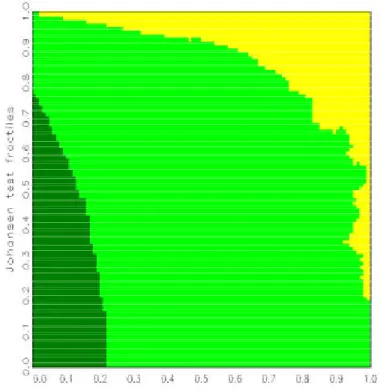
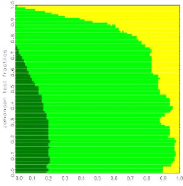
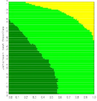
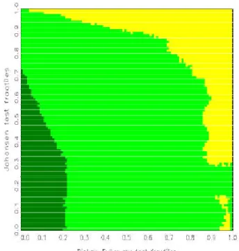
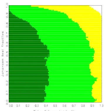
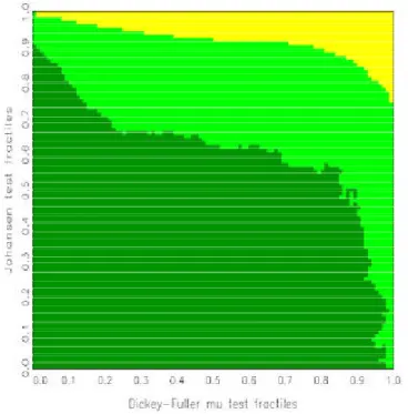
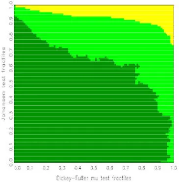
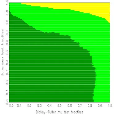
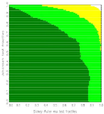
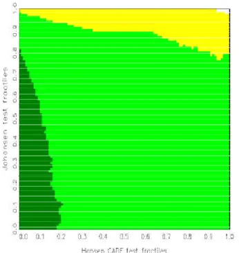
3.4 Decision boundaries

The aim of the simulations is to establish areas where £

and £

are pre- ferred, given the observed test statistics, for example the Dickey-Fuller statistic »

and the Johansen statistic »

. In line with usual Bayes testing, a hypothesis is preferred whenever its probability given the data, or rather the pair (»

; »

), exceeds 1/2. Based on a suggestion by Hatanaka (1996), the plane (»

; »

) is not drawn directly but both statistics are coded by the respective fractiles under their null distributions. For the calculation of these fractiles, two options are available. Firstly, asymptotic distributions can be used, such as Â

for the Johansen test, which is particularly attractive if closed forms of the distribution functions exist, or alternatively simulated distributions that are drawn for the speci…ed sample size. Secondly, sim- ulated …nite-sample fractiles can be obtained directly from the part of the simulated ‘posteriors’ that have been drawn from the respective null model.

As theoretical and asymptotic null distributions may not be valid in …nite samples and in the presence of a variety of nuisance parameters that are randomized for both hypothesis priors, the latter option is attractive. We tentatively used both speci…cations and found the deviations between them to be acceptably small. Finally, the former option was adopted, as a map for the sample fractiles would require any potential user of the map to re-run our speci…c simulation design. On the other hand, fractiles of the Â

distribution exist in a closed form and fractiles of the Dickey-Fuller distribution can easily be simulated.

In detail, a large number of trajectories are randomly drawn, that is, with randomized nuisance, from £

as well as from £

and the empirical distri- butions of »

j £

and of »

j £

are seen as the respective null distribution.

Empirical fractiles are stored at a grid of 0.01, which gives 100

= 10; 000 discretized cases of (»

; »

). If more of these pairs within a ‘bin’ stem from a certain hypothesis, it follows that the conditional probability of that hy- pothesis exceeds the conditional probability of the rival hypothesis. The bin is then marked as ‘belonging to £

’ with j = A; B.

For a large number of replications, the areas are typically connected and are separated by smooth boundary curves. Denoting the null fractiles for the statistics »

and »

by p

and p

for 0 · x; y · 1, one observes that P f (»

; »

) 2 ¡

p

; p

¢ £ ¡

p

; p

¢ j £

g may be small for

both j = A; B for some k; l. In other words, for relatively small numbers

of replications, some bins are poorly populated. Then, no reliable evalu-

ation of the posteriors of interest P f £

j (»

; »

) 2 ¡

p

; p

¢ £

¡ p

; p

¢ g will be possible. In particular, there will be little in- formation on whether the posterior probability of £

or £

is larger. Con- sequently, the simulated boundaries may look blurred and unreliable in the areas where the marginal density of (»

; »

) is low. The problem is similar to the one of density estimation and hence calls for solutions known from the related literature, in particular for kernel smoothing .

With kernel smoothing, the value in the bin (k

; l

) is replaced by a weighted average over an area of neighboring bins that are centered at (k

; l

).

Formally, the function value f (k

; l

) for a function de…ned on f 1; : : : ; n

g £ f 1; : : : ; n

g is replaced by its smoothed version

f

(k

; l

) =

k0

X

l0

X

w(k; l )f (k; l) :

Here, n

denotes the number of grid values, in this case n

= 100. Some modi…cations have to be conducted for indices outside the range f 1; : : : ; n

g . After some experimentation with kernel functions and areas, it was decided to use the kernel function

w (k; l) = W

1 + j k ¡ k

j + j l ¡ l

j ; k

¡ n

· k · k

+n

; l

¡ n

· l · l

+n

with the area size parameter n

, which was set at the minimum value that achieved smooth boundaries. The value W is set according to the requirement

1 =

k0

X

l0

X

w(k; l):

Note that it is not binding in this case, as the f

values from both hypotheses are used for a bilateral comparison only. Whenever the indices violate the range, the weights of non-existing observations are set to zero and hence an asymmetric version of the kernel is used, with W properly de…ned.

Kernel smoothing can be applied to the original counts of entries in the

bins or to the empirical posterior probabilities of hypotheses. In benchmark

cases with known outcome, it was found that smoothing the probabilities

created less distortions than smoothing the entry numbers, hence this op-

tion was chosen. As an indicator of such distortions, the unsmoothed maps

were compared to the smoothed maps. While the smoothed versions should

show connected and plausible boundaries, these boundaries should be lo- cated close to the boundaries that are approximately recognizable from the unsmoothed versions. In other words, there should not be systematic shifts from ‘free-hand’ boundaries to smoothed boundaries. Unfortunately, such shifts are likely whenever there are locally large increases in the function values. Smoothing the probability ratios implied only a tolerable tendency toward such shifts.

In the presented charts, which were generated using the GAUSS software package, the two preference areas for hypothesis £

and £

are separated by the decision boundary. The preference areas are indicated by di¤erent colors. Furthermore, we chose to divide the decision area for £

by a further boundary at the location where the posterior probability for £

is 0.75. In the region to the southwest of this secondary boundary, support for £

can be regarded as ‘strong’. This area is marked in the darkest shade. In some cases, we also show the analogous boundary for the probability for £

of 0.75.

Then the area to the northeast with strong preference for £

is marked in pure white.

4 Results of the simulations

For the …rst experiment, »

is speci…ed as the Johansen statistic as described above, without augmentation and assuming a bivariate …rst-order vector au- toregression, just as the one that actually generates the data. The unit-root statistic »

is speci…ed as the Dickey-Fuller statistic with a constant term included (Dickey-Fuller’s ‘¹–test statistic’), with p ¡ 1 augmenting lags.

The actual value of p was found by an AIC search with the upper bound of 5 on the lag order. Due to the bivariate generating model, univariate autore- gressions are imperfect speci…cations, hence augmentation was considered to make up for this defect. It was found that the DF statistic without aug- mentation is a very bad statistic and that its implied null distribution in the experiment is very di¤erent from the one tabulated in the literature. With an augmentation determined from the sample, the correspondence improves.

It was also found that the trend-augmented Dickey-Fuller statistic yields a relatively poor performance that cannot keep pace with the Johansen test.

This is probably due to the fact that the Johansen statistic uses information on the deterministic part of the generating model while the ‘¿ –test statistic’

would not. The implied Johansen null distribution comes quite close to the

theoretical Â

, with a small negative size bias. Sample size was varied over T = 50, 100, 200. The number of replications was always 2 £ 10

, i.e., 10

for each of the hypotheses £

and £

.

For …rst-order autoregressions (see Section 3.2), Figures 1–4 show the sim- ulated contour maps. The interpretation of the fractiles is slightly di¤erent for the two statistics. The Dickey-Fuller statistic »

rejects for large neg- ative values (the lower tail), which therefore conform to hypothesis A where the unit vector cointegrates. The Johansen statistic »

rejects for large pos- itive values (the upper tail), which therefore rather conform to hypothesis B where the cointegrating vector di¤ers from the unit vector. Therefore, one would predict a preference for hypothesis A in a south-west vertical band and a preference for hypothesis B in a north-east horizontal band.

The maps reveal that the principal information for the decision is provided by the Johansen statistic »

that becomes critical if it falls into the upper decile of the assumed Â

null distribution. The main contour is sloping only gently toward the east until the Dickey-Fuller statistic »

reaches some upper fractile. The position of this fractile point varies with the sample size and may be at 0.8 for T = 100. To the east of this value, hypothesis B is generally preferred. Notice that such large values of »

are usually taken as evidence on instability, locally ‘explosive’ behavior, or mis-speci…cation. A traditional application of the Dickey-Fuller test would locate the critical values in the lower fractiles.

The approximate visual impression from decision-bound curves as shown in Figures 1–4 can serve a useful purpose in evaluating the relative strength of tests. If in the largest part of the diagram the boundary curve runs parallel to an axis, the statistic displayed on that axis is of little value as compared to the rival statistic. If the boundary curve runs in a di¤erent direction, both statistics should be combined in order to improve upon the overall decision.

Particularly if the contour runs at a 45 degree slope, a common rule of thumb should be followed by directly comparing the p–values of both tests. If the

‘corners of con‡ict’, in this case the north-west and the south-east corner,

are intersected by the boundary curve, usage of a joint test is supported. If

these corners are allotted clearly on the basis of one of the two statistics,

usage of just one test statistic su¢ces. Traditional hypothesis testing can be

represented by two straight lines: a horizontal line at 0.9 or 0.95 separates

the preference area for hypothesis A beneath the line from an area above

the line where ‘the test rejects £

’; a vertical line at 0.05 or 0.1 separates

the preference for hypothesis B to its right from the left area where ‘the test

rejects £

’. The practitioner is not o¤ered a decision for the large south-east and the small north-west corners where the rejections are in con‡ict.

As a kind of sensitivity analysis, the prior distribution was modi…ed in Figure 3 such that the o¤-diagonal elements in T were set to Cauchy random numbers instead of normal random numbers, as in the other experiments.

The larger variation of behavior caused by the Cauchy distribution requires stronger smoothing. The vertical boundary seen in Figure 2 disappears, so that the suggested decision now relies only on the Johansen statistic. Oth- erwise, the structure of the decision map is very similar to the basic exper- iment. From this and other unreported sensitivity experiments, it has been concluded that the choice of the prior distribution does not a¤ect the main results too much, as long as the modi…cation hits both hypotheses symmet- rically. In further unreported experiments, similar e¤ects were encountered by increasing ¾

=¾

while maintaining normality.

For the important design of Figure 2, i.e., the Dickey-Fuller ¹ test and T = 100, the e¤ect of deterministic termes was also studied. Figure 5 shows the e¤ects of a randomized added drift with ¾

= 1. This modi…cation is apparently bene…cial for the discriminatory power of the Dickey-Fuller statistic »

, as the boundary now runs vertically at the upper decile of its null distribution, unless »

reaches large values. It should be noted , however, that the eastern part of the diagram is still sparsely populated and that the suggested critical value is in the upper tails and not in the lower tails, which would be the traditional approach of unit-root testers. The variant con…rms that the decision should be based on assigning a much larger weight to the statistic »

and to re-consider this decision only when the statistic »

points to a data-generating process in the explosive region. We also note that the north-east corner now yields a high posterior probability for hypothesis B.

Recalling that such pairs correspond to rejection of the self-cointegration null jointly with large and positive Dickey-Fuller statistics. Relative to the maps without drift, there are increased areas where preference for one of the two hypotheses exceeds 0.75. The added trends permit more accurate decisions, therefore decreasing global risk.

For second-order autoregressions (see Section 3.3), the Figures 6-8 are

obtained. These are generally similar to the …rst-order cases. The area

with strong preference for hypothesis A increases, which points to a steeper

reaction along the decision contour and therefore a decrease in risk. With

increased sample size, the evidence provided by Dickey-Fuller statistics

in the upper tails of their null distribution becomes more reliable, hence

the hypothesis B area stretches southward from its north-eastern habitat.

Notwithstanding these minor di¤erences between …rst-order and second-order autoregressions, the main message is the same. The optimal decision should rely mainly on the Johansen test statistic. Large »

values indicate the validity of hypothesis B, with ‘large’ de…ned as the upper decile of the Â

null distribution. For conspicuously low or high values of »

, this decision should be adapted. These basic simulations are contrasted with a variant with randomized drift in Figure 9. The e¤ect of the added trends are similar to those for the …rst-order autoregression. Global risk decreases and preference for hypothesis B is restricted to the north-east corner.

Figures 10–12 are based on the CADF test that was investigated by

Hansen, though in a slightly di¤erent model frame. Because this test uses

multivariate information such as the Johansen test, one may expect a rela-

tive improvement of performance relative to the ADF test. For T = 50, the

diagram shown in Figure 10 was obtained. The separating contour is almost

horizontal and again gives preference to the Johansen statistic. However,

the secondary contour with a posterior probability of 0.75 for hypothesis A

is now vertical at a p–value that comes close to those used in traditional

statistical analysis. In other words, basing the decision on the Johansen

statistic only implies a substantial risk of an incorrect choice of hypothesis A,

although the data actually stem from hypothesis B. Nevertheless, the risk of

an incorrect decision for hypothesis B in the large south-east region is larger,

hence the ‘non-rejection’ according to the CADF test should be ignored. For

T = 100, Figure 11 is obtained, which is similar and just shows a slight

gain of the preference area for hypothesis B in the east, i.e., for uncommonly

large CADF statistics. The expansion of the preference area for hypothesis

B continues as the sample is increased to T = 200. This experiment is shown

as Figure 12. Note that the increase in sample information has only small

bene…ts for the targeted decision, as the 0.75 support area for hypothesis A

hardly changes. Apparently, most of the additional information is exploited

by the CADF statistic that now helps in discriminating among the ‘pseudo-

explosive’ trajectories that yield a large DF statistic. A similar feature was

observed for the univariate DF statistic (see Figures 1, 2, and 4), hence the

e¤ect of incorporating multivariate information in the CADF test fails to

convince.

5 Summary and conclusion

In a series of simulation experiments, the optimum decision that can be based on a joint application of two di¤erent unit-root tests was evaluated.

The method is innovative and is based on the principle of Bayes testing. In order to randomize the nuisance parameters, i.e., those parameters that are neither characteristic nor distinctive in de…ning a hypothesis, these are given a regular prior distribution. This prior distribution is designed to exhaust all possible models under any of the two hypotheses under investigation.

Then, the same number of stochastic simulations are conducted under either hypothesis. Finally, the null fractiles are evaluated and the actual outcomes are compared to these null fractiles for both tests.

Some unreported decision contour plots have shown that the Dickey- Fuller test with a trend regressor is not useful for joint testing with a Johansen restriction test in the given model frame where a cointegrating rank of one has been established or assumed. For the Dickey-Fuller speci…cation without a trend regressor and for the modi…ed test that was suggested by Hansen, the situation is di¤erent. The main features are summarized below:

1. In most contour plots, the main or 0.5 decision contour suggests bas- ing the principal decision on the Johansen statistic. Signi…cant Jo- hansen statistics should usually be taken as evidence against self- cointegration or stationarity of the investigated component.

2. The contour shows a gentle downward slope, however, and the princi- pal decision should therefore be re-considered in the presence of very negative unit-root statistics. The tested variable is likely to be station- ary if, for example, the Johansen statistic is in its upper decile but the unit-root statistic is in its lower decile. The exact position of the decision contour varies with the sample size, the intensity of short-run memory, and the deterministic part. The second e¤ect was investigated by varying the lag order of the generating model. Adding determinis- tic parts usually admits a sharper decision and thus decreases decision risk.

3. The ADF or CADF statistic becomes conspicuous when it indicates

stationarity (‘rejects’) and when it indicates explosiveness, i.e., is in its

upper decile. Explosive values of unit-root statistics imply a high risk

of mis-classi…cation. In smaller samples, such values suggest lowering the critical values for the Johansen test, e.g., from 0.9 to 0.8. In larger samples, they indicate a unit root in the tested component variable.

The decision problem is of importance to practitioners who analyze eco- nomic data sets on the basis of widely available software that enables them to conduct the popular Johansen procedure as well as traditional unit-root tests. In many cases, they …nd con‡icting evidence and often reach a …nal conclusion on the basis of conjectures and ad hoc decisions, which may seem unsatisfactory. This motivates further work that is particularly directed at helping practitioners who face such empirical puzzles. The method can be re…ned in several directions, such as higher system dimension, varying the search method for the correct lag speci…cation, or more sophisticated deter- ministic structures. In all such extensions, the outlined ‘global’ Bayes-test method will be able to reveal features that remain unnoticed in the tradi- tional ‘local’ frequentist framework with its …xed designs of data-generating processes. Of course, this observation should not discourage traditional power studies that focus on local or large-sample (asymptotic) features that nec- essarily remain out of the focus of the global approach. Hence, the two approaches should rather be seen as complementary and not as substitutes.

References

[1] Charemza, W.W., and E.M. Syczewska (1998) ‘Joint application of the Dickey-Fuller and KPSS tests’, Economics Letters 61, 17–21.

[2] Dickey, D.A., and W.A. Fuller (1979) ‘Distribution of the esti- mators for autoregressive time series with a unit root’, Journal of the American Statistical Association 74, 427–431.

[3] Hansen, B.E. (1995) ‘Rethinking the Univariate Approach to Unit Root Testing’, Econometric Theory 11, 1148–1171.

[4] Hatanaka, M. (1996) Time-Series-Based Econometrics: Unit Roots and Co-Integration. Oxford University Press.

[5] Horvath, M.T.K., and M.W. Watson (1995) ‘Testing for cointegra-

tion when some of the cointegrating vectors are prespeci…ed’, Economet-

ric Theory 11, 984–1014.

[6] Johansen, S. (1995) Likelihood-Based Inference in Cointegrated Vector Autoregressive Models. Oxford University Press.

[7] Johansen, S., and K. Juselius (1995) ‘Testing structural hypotheses in a multivariate cointegration analysis of the PPP and the UIP of UK’, Journal of Econometrics 53, 211–244.

[8] Kunst, R.M., and M. Reutter (2002) ‘Decisions on seasonal unit roots’. Journal of Statistical Computation and Simulation. forthcoming.

[9] Lee, H.S. (1992) ‘Maximum Likelihood Inference on Cointegration and Seasonal Cointegration’, Journal of Econometrics 54, 1–47.

[10] Maddala, G.S., and I.M. Kim (1998) Unit Roots, Cointegration, and Structural Change. Cambridge University Press.

[11] Pantula, S.G. (1989) ‘Testing for unit roots in time series data’, Econometric Theory 5. 256–271.

[12] Rahbek, A., and R. Mosconi (1999) ‘Cointegration rank inference with stationary regressors in VAR models’, Econometrics Journal 2, 76–91.

[13] Tanaka, K. (1996) Time Series Analysis: Nonstationary and Nonin-

vertible Distribution Theory. Wiley.

Figures

Figure 1: Boundary of optimum decision areas for T = 50. Dickey-Fuller ¹ on

the x–axis, Johansen on the y–axis. First-order autoregression. Smoothing

constant is 31.

Figure 2: Boundary of optimum decision areas for T = 100. Dickey-Fuller ¹

on the x–axis, Johansen on the y–axis. First-order autoregression. Smooth-

ing constant is 33.

Figure 3: Boundary of optimum decision areas for T = 100. Dickey-Fuller

¹ on the x–axis, Johansen on the y–axis. First-order autoregression with

Cauchy-Jordan priors. Smoothing constant is 43.

Figure 4: Boundary of optimum decision areas for T = 200. Dickey-Fuller ¹

on the x–axis, Johansen on the y–axis. First-order autoregression. Smooth-

ing constant is 39.

Figure 5: Boundary of optimum decision areas for T = 100. Dickey-Fuller

¹ on the x–axis, Johansen on the y–axis. First-order autoregression with

random drift. Smoothing constant is 25.

Figure 6: Boundary of optimum decision areas for T = 50. Dickey-Fuller ¹ on

the x–axis, Johansen on the y–axis. Second-order autoregression. Smoothing

constant is 15.

Figure 7: Boundary of optimum decision areas for T = 100. Dickey-Fuller

¹ on the x–axis, Johansen on the y–axis. Second-order autoregression.

Smoothing constant is 13.

Figure 8: Boundary of optimum decision areas for T = 200. Dickey-Fuller

¹ on the x–axis, Johansen on the y–axis. Second-order autoregression.

Smoothing constant is 25.

Figure 9: Boundary of optimum decision areas for T = 100. Dickey-Fuller

¹ on the x–axis, Johansen on the y–axis. Second-order autoregression with

random drift. Smoothing constant is 25.

Figure 10: Boundary of optimum decision areas for T = 50. Hansen’s covariate-augmented Dickey-Fuller ¹ on the x–axis, Johansen on the y–axis.

First-order autoregression. Smoothing constant is 19.

Figure 11: Boundary of optimum decision areas for T = 100. Hansen’s covariate-augmented Dickey-Fuller ¹ on the x–axis, Johansen on the y–axis.

First-order autoregression. Smoothing constant is 35.

Figure 12: Boundary of optimum decision areas for T = 200. Hansen’s covariate-augmented Dickey-Fuller ¹ on the x–axis, Johansen on the y–axis.

First-order autoregression. Smoothing constant is 35.