Approaches for the Joint Evaluation of Hypothesis Tests: Classical Testing, Bayes Testing, and Joint Confirmation

IHS Economics Series Working Paper 177

September 2005

Approaches for the Joint Evaluation of Hypothesis Tests: Classical Testing, Bayes Testing, and Joint Confirmation

Robert M. Kunst

Impressum Author(s):

Robert M. Kunst Title:

Approaches for the Joint Evaluation of Hypothesis Tests: Classical Testing, Bayes Testing, and Joint Confirmation

ISSN: Unspecified

2005 Institut für Höhere Studien - Institute for Advanced Studies (IHS) Josefstädter Straße 39, A-1080 Wien

E-Mail: o ce@ihs.ac.atffi Web: ww w .ihs.ac. a t

All IHS Working Papers are available online: http://irihs. ihs. ac.at/view/ihs_series/

This paper is available for download without charge at:

https://irihs.ihs.ac.at/id/eprint/1652/

177 Reihe Ökonomie Economics Series

Approaches for the Joint Evaluation of Hypothesis Tests:

Classical Testing, Bayes Testing, and Joint Confirmation

Robert M. Kunst

177 Reihe Ökonomie Economics Series

Approaches for the Joint Evaluation of Hypothesis Tests:

Classical Testing, Bayes Testing, and Joint Confirmation

Robert M. Kunst September 2005

Institut für Höhere Studien (IHS), Wien

Institute for Advanced Studies, Vienna

Contact:

Robert M. Kunst

Department of Economics and Finance Institute for Advanced Studies Stumpergasse 56

1060 Vienna, Austria and

University of Vienna Department of Economics Brünner Straße 72 1210 Vienna, Austria

email: robert.kunst@univie.ac.at

Founded in 1963 by two prominent Austrians living in exile – the sociologist Paul F. Lazarsfeld and the economist Oskar Morgenstern – with the financial support from the Ford Foundation, the Austrian Federal Ministry of Education and the City of Vienna, the Institute for Advanced Studies (IHS) is the first institution for postgraduate education and research in economics and the social sciences in Austria.

The Economics Series presents research done at the Department of Economics and Finance and aims to share “work in progress” in a timely way before formal publication. As usual, authors bear full responsibility for the content of their contributions.

Das Institut für Höhere Studien (IHS) wurde im Jahr 1963 von zwei prominenten Exilösterreichern – dem Soziologen Paul F. Lazarsfeld und dem Ökonomen Oskar Morgenstern – mit Hilfe der Ford- Stiftung, des Österreichischen Bundesministeriums für Unterricht und der Stadt Wien gegründet und ist somit die erste nachuniversitäre Lehr- und Forschungsstätte für die Sozial- und Wirtschafts- wissenschaften in Österreich. Die Reihe Ökonomie bietet Einblick in die Forschungsarbeit der Abteilung für Ökonomie und Finanzwirtschaft und verfolgt das Ziel, abteilungsinterne Diskussionsbeiträge einer breiteren fachinternen Öffentlichkeit zugänglich zu machen. Die inhaltliche Verantwortung für die veröffentlichten Beiträge liegt bei den Autoren und Autorinnen.

Abstract

The occurrence of decision problems with changing roles of null and alternative hypotheses has increased interest in extending the classical hypothesis testing setup. Particularly, confirmation analysis has been in the focus of some recent contributions in econometrics.

We emphasize that confirmation analysis is grounded in classical testing and should be contrasted with the Bayesian approach. Differences across the three approaches – traditional classical testing, Bayes testing, joint confirmation – are highlighted for a popular testing problem. A decision is searched for the existence of a unit root in a time-series process on the basis of two tests. One of them has the existence of a unit root as its null hypothesis and its non-existence as its alternative, while the roles of null and alternative are reversed for the other hypothesis test.

Keywords

Confirmation analysis, decision contours, unit roots

JEL Classifications

C11, C12, C22, C44.

Contents

1 Introduction 1

2 Pairs of tests with role reversal of hypotheses 2

2.1 The general decision problem ... 2

2.2 Decisions in the classical framework ... 3

2.3 Joint confirmation ... 4

2.4 Bayes tests ... 5

3 A graphical comparison of three methods 6 4 Testing for unit roots in time series 10

4.2 Bayes-test experiments ... 13

4.3 An application to economics data ... 21

5 Summary and conclusion 22

References 24

1 Introduction

The occurrence of decision problems with role reversal of null and alternative hypotheses has increased the interest in extensions of the classical hypothesis testing setup. Particularly, confirmation analysis has been in the focus of some recent econometric works (see Dhrymes, 1998, Keblowski and Welfe, 2004, among others). This paper analyzes the contribution of confirmation analysis against the background of the more general statistical decision problem, and compares it to alternative solution concepts. The focus is on the decision for a unit root in time-series processes.

In this and in comparable situations, the basic difficulty of traditional hypoth- esis testing is that pairs of tests may lead to a contradiction in their individual results. The role reversal of null and alternative hypothesis prevents the tradi- tional construction of a new test out of the two components that may dominate individual tests with regard to power properties. The existing literature appears to suggest that conflicting outcomes indicate possible invalidity of the maintained hypothesis and therefore imply ‘no decision’ (e.g., see Hatanaka, 1996). In em- pirical applications, the ad hoc decision on the basis of comparing p—values is also widespread.

In a simplified interpretation, confirmation analysis (Charemza and Syczewska, 1998, Keblowski and Welfe, 2004, Dhrymes, 1998) suggests to select one of the two hypotheses as the overall null, thereby apparently resolving the conflict.

An obvious difficulty of this approach is that a ‘generic’ alternative of one of the component tests is condensed to a lower-dimensional null by choosing specific parts of the alternative. This selection may seem artificial. A logical drawback is also that the confirmation test follows the classical asymmetry of one of the component tests, while the basic problem reveals a symmetric construction prin- ciple. If the basic problem clearly indicated the choice of null and alternative, the application of a test with role reversal would not be adequate at all.

A different and completely symmetric solution is Bayes testing. It is well known from the literature on statistical decision theory (Lehmann and Ro- mano, 2005, Ferguson, 1967, Pratt et al., 1995) that Bayes tests define a complete class for any given loss function, in the sense that any other test is dominated by a Bayes test. However, Bayes tests require the specification of elements such as loss functions and prior distributions that are often regarded as subjective.

This paper adopts a Bayesian viewpoint and presents Bayes-test solutions to the unit-root decision problem in a graphical manner in rectangles of null fractiles. In a related decision problem on the existence of seasonal unit roots, a similar approach was introduced by Kunst and Reutter (2002). Using some sensitivity checks by varying prior distributions, the relative benefits with regard to loss criteria can be compared to the classical and also to the confirmation approach. The graphical representations allow a convenient simplification and

1

visualization of traditional Bayes tests by focusing exclusively on the observed test statistics.

Section 2 analyzes the three approaches to joint testing with reversal of hy- potheses that have been presented in the literature: classical ideas, joint confir- mation (Charemza and Syczewska, 1998, CS), and Bayes tests. We review the problem as it is viewed in the more classical (see, for example, Lehmann and Romano, 2005) or in the more Bayesian tradition (see, for example, Ferguson, 1967, or Pratt et al., 1995).

Section 3 highlights the differences across the three approaches graphically and generally. In Section 4, we consider an application in time-series analysis, viz. the statistical testing problem that was considered by CS and Keblowski and Welfe (2004). A decision is searched for the existence of a unit root in a time-series process on the basis of two tests. One of them has the existence of a unit root as its null hypothesis and its non-existence as its alternative, while the roles of null and alternative are reversed for the second hypothesis test. Section 5 concludes.

2 Pairs of tests with role reversal of hypotheses

2.1 The general decision problem

We consider statistical decision problems of the following type. The maintained model is expressed by a parameterized collection of densities. The parameter space Θ is possibly infinite-dimensional. Based on a sample of observations from an unknown member θ ∈ Θ, a decision is searched on whether θ ∈ Θ

or θ ∈ Θ

, with Θ

∪ Θ

= Θ and Θ

∩ Θ

= ∅ . The event { θ ∈ Θ

} is called the null hypothesis, while { θ ∈ Θ

} is called the alternative hypothesis. If θ ∈ Θ

, ‘the null hypothesis is correct’, while for θ ∈ Θ

the ‘alternative is correct’. While the parameter space Θ may be infinite-dimensional, classification to Θ

and Θ

should rely on a finite-dimensional subspace or ‘projection’. If the finite-dimensional projection of θ is observed, θ can be allotted to Θ

or Θ

with certainty. The occurrence of non-parametric nuisance is crucial for the problem that we have in mind.

Example. An observed variable X is a realization of an unknown real-valued probability law with finite expectation. Θ

may consist of those probability laws that have E X = 0, while Θ

may be defined by E X 6 = 0. Decision is searched for a one-dimensional parameter, while Θ is infinite-dimensional. ¤

A characteristic feature of statistical decision problems is that θ is not ob- served. If θ were observed, this would enable perfect classification. This perfect case can be envisaged as incurring zero loss, in line with the usual concept of the loss incurred by a decision. Typically, a sample of observations for a random vari- able X is available to the statistician, where the probability law of the random

2

variable is governed by a density f

(.). In many relevant problems, observing an infinite sequence of such observations allows to determine θ almost surely and therefore to attain the loss of zero that accrues from direct observation of θ.

Typically, finite samples will imply non-zero loss. Following classical tradition, incorrect classification to Θ

is called a type II error, while incorrect classification to Θ

is called a type I error. For many decision problems, testing procedures can be designed that take both type I and the type II errors to zero probability, as the sample grows to infinity. We note, however, that hypothesis tests with ‘fixed significance level’ do not serve this aim.

2.2 Decisions in the classical framework

Assume τ

is a test statistic for the decision problem with the null hypothesis θ ∈ Θ

and the alternative θ ∈ Θ

, while τ

is a test statistic with reversed null and alternative hypotheses. A hypothesis test using τ

will usually be designed to have a pre-assigned upper bound α for the probability of a type I error P

(θ), such that P

(θ) ≤ α for all θ ∈ Θ

. Furthermore, the test will be designed such that the probability of a type II error P

(θ) will be minimized in some sense for θ ∈ Θ

. While P

(θ) will critically depend on θ ∈ Θ

in finite samples, test consistency requires P

(θ) → 0 as n → ∞ for every θ ∈ Θ

.

By construction, the error probabilities for the test defined by τ

will have reversed properties. Therefore, a decision based on the two individual tests and common α will have a probability of incorrectly selecting Θ

bounded by α, and the same will be true for the probability of incorrectly selecting Θ

. First assume independence of the two test statistics. Then, for some parameter values, these error probabilities may be close to α (1 − α), while for others they may be much lower. If both individual tests are consistent, both error probabilities should converge to zero, as the sample size increases. Thus, the joint test achieves full consistency in the sense of both P

(θ) → 0 for θ ∈ Θ

and P

(θ) → 0 for θ ∈ Θ

. Even allowing for some dependence of the two test statistics are dependent will not invalidate the argument. Full consistency, which is not typical for classical tests, comes at the price that the true significance level of the test is less than α for all sample sizes.

A drawback is that the decision for Θ

is implied only if the test based on τ

‘fails to reject’ and the test based on τ

‘rejects’. If the τ

test ‘rejects’ and the τ

test ‘fails to reject’, a decision for Θ

is suggested. In cases of double rejection or double non-rejection, no coercive decision is implied. Allotting these parts of the sample space arbitrarily to the Θ

or the Θ

decision areas would express a subjective preference toward viewing the hypothesis design of one of the two individual tests as the correct one and, therefore, the other test design as ‘incorrect’.

Some, with Hatanaka(1996), interpret conflicting outcomes as indicating invalidity of the maintained hypothesis Θ. While this may be plausible in some

3

problems, it may require an approximate idea of possible extensions of the main- tained model Θ

⊃ Θ. Clearly, in a stochastic environment, contradictory out- comes will not have a probability of zero, whatever has been the data-generating model. We assume that a complete decomposition of the sample space into two regions Ξ

(preference for Θ

) and Ξ

(preference for Θ

) is required. This can be achieved by basing the choice on comparing the p—values of individual tests.

If both individual tests reject, the rejection with the larger p—value is ignored.

Similarly, if both tests ‘do not reject’, the lower p—value is taken as indicating rejection. It appears that this casual interpretation of p—values is quite common in practice. By construction, the decision rule ignores any dependence among τ

and τ

.

2.3 Joint confirmation

Let the acceptance regions of the two tests using τ

and τ

be denoted as Ξ

and Ξ

, and similarly their rejection regions as Ξ

and Ξ

. Then, one may consider basing the decomposition (Ξ

, Ξ

) on bivariate intervals. It is straight forward to allot the ‘clear’ cases according to

Ξ

∩ Ξ

⊂ Ξ

,

Ξ

∩ Ξ

⊂ Ξ

. (1) In the remaining parts of the sample space, the two statistics seemingly point to different conclusions. Seen as tests for ‘null’ hypotheses Θ

and Θ

, allotting these parts to Ξ

or Ξ

may result in ‘low power’ or in violating the ‘risk level’

condition.

‘Joint confirmation hypothesis’ testing or ‘confirmatory analysis’, according to CS, targets a probability of joint confirmation (PJC), which is defined as ‘deciding for Θ

, given the validity of Θ

’. Consider the error integrals

P

(θ) = Z

Ξ1

f

(x) dx, P

(θ) = Z

Ξ0

f

(x) dx, (2) Let us view the joint test as having Θ

as its ‘null’ and Θ

as its ‘alternative’. For θ ∈ Θ

, P

(θ) is the probability of a type II error, while, for θ ∈ Θ

, P

(θ) is the probability of a type I error. CS define the PJC as P

(θ) for some θ ∈ Θ

. Since P

(θ) = 1 − P

(θ), the PJC simply is one minus the type II error probability for a specific θ ∈ Θ

. The error integral P

(θ) is evaluated for some θ, which are members of the alternative for the test construction τ

and members of the null hypothesis for the construction of τ

. Therefore, P

(θ) expresses the probability that τ

would wrongly accept its null and τ

would correctly accept its null if the tests were used individually. If (τ

, τ

) is used jointly, it is the probability of an incorrect decision for some given θ ∈ Θ

.

4

Usually, there is a manifold of pairs (τ

, τ

) such that (τ

, τ

) = (τ

, τ

) implies the condition P

(θ) = 1 − α for a given α. Among them, joint confirmation selects critical points (τ

, τ

) by the condition that P

(θ) coincide for the two component tests that build on individual τ

and corresponding τ

. While this superficially looks like a Bayesian critical point, where the probabilities of Θ

and Θ

coincide, no probability of hypotheses is used, as the procedure is built in the classical way, where hypotheses do not have probabilities. While an informal Bayesian interpretation of p —values may interpret them as such probabilities, a genuine Bayes test determines critical points by comparing probabilities for Θ

and Θ

, not two measures of probability for Θ

. An apparent advantage of joint confirmation is, however, that it avoids the Bayesian construction of weighting functions.

2.4 Bayes tests

The occurrence of an apparent contradiction by two individual hypothesis tests has a relatively simple solution in Bayesian statistics. The admissible parameter space is defined as Θ

∪ Θ

and the remainder is a priori excluded, according to the statement of the decision problem. After fixing weight functions h

and h

on the hypotheses and a loss criterion g, the decision problem can be subjected to computer power and yields a solution that is optimal within the pre-defined set of admissible decompositions (Ξ

, Ξ

). For example, one may restrict attention to decompositions that are based on the test statistics (τ

, τ

) and on bivariate intervals.

The Bayesian setup to testing problems assumes weighting functions h

and h

on the respective parameter spaces Θ

and Θ

, which can be interpreted as probability densities. While a usual interpretation of h

and h

is that they represent a priori probabilities of parameter values, it is not necessary to adopt this interpretation for Bayes testing. If the sample space, for example R

for sample size n, is partitioned into two mutually exclusive subsets Ξ

and Ξ

, such that X ∈ Ξ

implies deciding for θ ∈ Θ

, the probability of a type I error is P

(θ) for a given member θ ∈ Θ

. The Bayes weighting scheme allows to evaluate

L

(h

, Ξ

) = Z

Θ0

Z

Ξ1

f

(x) dx h

(θ) dθ (3) as a measure for the ‘average’ type I error involved in the decision. Conversely, the integral

L

(h

, Ξ

) = Z

Θ1

Z

Ξ0

f

(x) dx h

(θ) dθ = Z

Θ1

P

(θ) h

(θ) dθ (4) represents the ‘average’ type II error involved. A Bayesian view of the decision problem is to minimize the Bayes risk

g ( L

(h

, Ξ

) , L

(h

, Ξ

))

5

= g µZ

Θ0

Z

Ξ1

f

(x) dx h

(θ) dθ, Z

Θ1

Z

Ξ0

f

(x) dx h

(θ) dθ

¶

(5) in the space of possible partitions of the sample space, for a given function g : R

→ R

. The function g is designed to express the afore-mentioned loss.

Therefore, g (0, 0) = 0 and monotonicity in both arguments are useful restric- tions. If for any θ ∈ Θ

no observed sample generated from that θ implies the incorrect decision Ξ

with k 6 = j, both arguments are zero and the loss is zero.

Zero Bayes risk can also be attained if incorrect decisions occur for subsets ˜ Θ

⊂ Θ

with h

= 0 or R

Θ˜j

h

dθ

= 0 only.

By construction, Bayes tests attain full consistency P

(θ) → 0 for θ ∈ Θ

and P

(θ) → 0 for θ ∈ Θ

by minimizing g( L

(h

, Ξ

) , L

(h

, Ξ

)) → 0, except on null sets of the measure that is defined by the weighting priors h

, h

. In a Bayesian interpretation, the classical approach is often viewed as allotting a strong relative implicit weight to Θ

in smaller samples, which makes way to a strong weight on Θ

as the sample size grows. This ‘weight’ refers to the corresponding derivatives g

and g

of the g function, not to the weighting priors h

and h

.

3 A graphical comparison of three methods

Assume the individual test using τ

rejects in the left tail of the range, while the test using τ

rejects in the right tail.

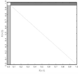
For an instructive comparison across the methods, first consider Figure 1.

Without restricting generality, we consider a situation where Θ

corresponds to the null of the test using τ

and to the alternative of the test using τ

. It is convenient to ‘code’ both tests in terms of their respective null distributions. In other words, the diagram is not drawn in the original coordinates (τ

, τ

) ∈ R

but rather in the fractiles (F

(τ

) , F

(τ

)) ∈ [0, 1]

for distribution functions F

and F

. Because distribution functions are monotonous transforms, the information remains identical for any such functions. However, it eases the interpretation of the diagrams if F

corresponds to the ‘null distributions’ of τ

, assuming that a distribution of τ

under its null hypothesis is (approximately) unique. In short, we label the axes by F

(τ

) and F

(τ

). Rejection by the test using τ

corresponds to F

(τ

) < α. In the following, we adopt the conventional level α = 0.05. If the test using τ

rejects and the test using τ

does not or the sample is in Ξ

∩ Ξ

, there is clear evidence in favor of hypothesis Θ

. Conversely, if the first test does not reject and the second test does so or the sample is in Ξ

∩ Ξ

, we have clear evidence in favor of Θ

. If both tests accept or reject, the evidence remains unclear. This fact is expressed by leaving the north-west and south-east regions white.

The diagonal line indicates the informal classical solution of allotting the undecided regions according to a simple comparison of p—values. If this procedure

6

is adopted, all points above the line are interpreted as preferring Θ

and those below the line as preferring Θ

.

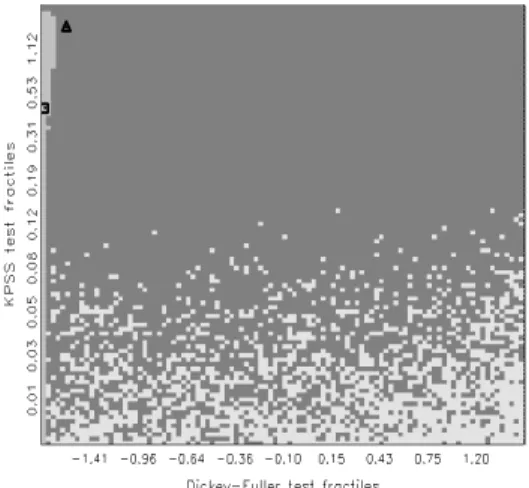
Figure 1: Classical decision following the joint application of two classical tests with switching null hypotheses. Axes are determined by the null distribution of τ

and the null distribution of τ

. Light gray area represents decisions in favor of Θ

, while the dark gray area corresponds to Θ

.

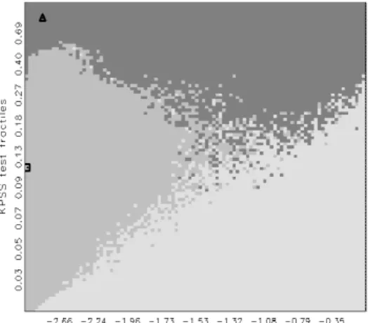
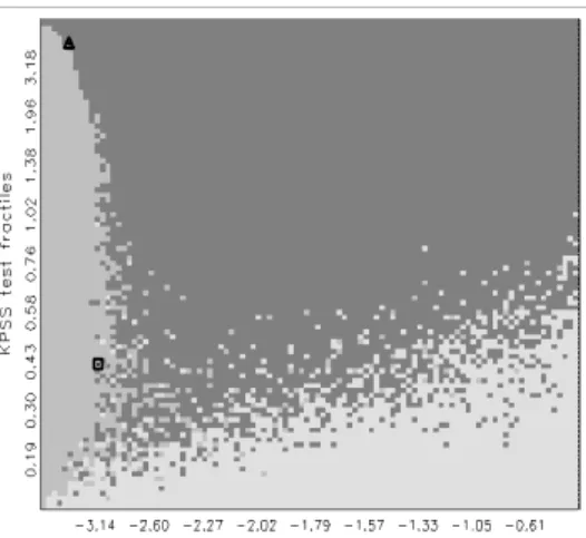
Next, consider Figure 2. It represents the decision of joint confirmation.

Rather than using the null distributions of the two test statistics τ

and τ

, we use here the null distribution of τ

but the alternative distribution of τ

and code the two test statistics accordingly. Usually, the alternative distribution does not exist, therefore one uses a representative element from the τ

alternative. If τ

rejects and τ

accepts, this is the ‘confirmation area’ of hypothesis Θ

. Its probability under the representative distribution from Θ

has a given probability α. Along the (x, 1 − x)—diagonal, individual rejection probabilities coincide, thus the corner point is selected.

A possible interpretation of the method’s focus on the north-east confirmation area is that the dark gray area favors Θ

, while the remaining area favors Θ

. The work of CS appears to support this interpretation by using a similar coloring of the four areas in a histogram plot. The interpretation is not coercive, however, and one may also forego a decision in conflicting cases, as in the classical rule of Figure 1. Then, joint confirmation becomes closer in spirit to reversing a classical test by replacing the original alternative by a point alternative, such that it becomes a convenient null. We refrain from this simplifying view, which is invalid in the classical tradition, and we view the joint confirmation decision according to Figure 2. In any case, the procedure is asymmetric, as confirming Θ

leads to a different solution from confirming Θ

. The choice of confirmed

7

hypothesis is not entirely clear. CS and Keblowski and Welfe (2004) choose the null of the more popular component test.

Figure 2: Joint-confirmation decision following the joint application of two clas- sical tests with switching null hypotheses. Axes are determined by the null dis- tribution of τ

and a representative alternative distribution of τ

. Light gray area represents decisions in favor of Θ

, while the dark gray area corresponds to Θ

.

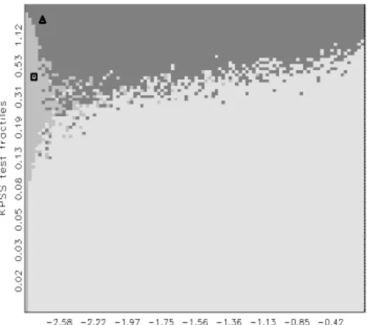
A typical outcome of a Bayes test is depicted in Figure 3. As in the clas- sical test in Figure 1, axes correspond to respective null distributions functions F

(x) = R

−∞

f

(z) dz. However, instead of a fixed density f

(z), we now use a weighted average R

Θj

f

(z) h

(θ) dθ of all possible null densities. Then, a sim- ulation with 50% Θ

and 50% Θ

distributions is conducted, where all kinds of representatives are drawn, according to weight functions h

and h

. Accord- ingly, a boundary can be drawn, where both hypotheses occur with the same frequency. Northeast of this decision contour, the hypothesis Θ

is preferred, while to the southwest the hypothesis Θ

is preferred. While the decision rests on a more informative basis than in the other approaches, the position of the curve is sensitive to the choice of h

and h

. In a fully Bayesian interpretation, the decision contour is defined as the set of all points τ

= (τ

, τ

) ∈ R

where P (Θ

| τ

) = P (Θ

| τ

), if Θ

have prior distributions of equal probability across hypotheses, i.e. P (Θ

) = P (Θ

), and the elements of the two hypotheses have prior probabilities according to the weight functions h

and h

. In the interpre- tation of the decision framework that we introduced in Section 2, the decision contour is the separating boundary of the two regions Ξ

and Ξ

, conditional on the restrictions that only such separations of the sample space are permitted that depend on the observed statistic τ

and on a loss function g (., .) that gives equal weight to its two arguments, such as g (x, y) = x + y.

8

Figure 3: Bayes-test decision following the joint application of two classical tests with switching null hypotheses. Axes are determined by weighted averages of null distributions of τ

and τ

. Light gray area represents decisions in favor of Θ

, while the dark gray area corresponds to Θ

.

The choice of h

and h

is undoubtedly important for the Bayes test, as are all types of prior distributions for Bayesian inference. There are several prescriptions for ‘eliciting’ priors in the Bayesian literature. To some researchers, elicitation should reflect true prior beliefs, which however may differ subjectively and are maybe not good candidates for situations with strong uncertainty regarding the outcome. Other researchers suggest to standardize prior distributions and, con- sequently, weight functions according to some simple scheme. Particularly for Bayes testing aiming at deriving decision contours, it appears to be a good idea to keep the weight functions flat close to the rival hypothesis. The tail behavior of the weight functions has less impact on the contours.

An important requirement is that the weighting priors are exhaustive in the sense that, for every θ ∈ Θ

, any environment containing θ, E (θ), should have non-zero weight h

(E (θ)) > 0. This ensures that open environments within Θ

appear with positive weight in L

(h

, Ξ

) or L

(h

, Ξ

) and, consequently, that the Bayes risk g converging to zero as n → ∞ implies full consistency. Informally, exhaustiveness means that, for any distribution within Θ there is a distribution

‘close’ to it that can be among the simulated draws.

Another important choice is the loss function g . The function g (x, y ) = x + y corresponds to the Bayesian concept of allotting identical prior weights to the two hypotheses under consideration. In line with the scientific concept of unbiased opinion before conducting an experiment and in a search for ‘objectivity’, it appears difficult to accept loss functions such as g (x, y) = (1 − κ) x + κy with κ 6 = 1/2. These functions are sometimes used in the Bayesian literature (for

9

example, see Pratt et al., 1995) and may represent prior preferences for one of the two hypotheses. Classical tests with fixed significance levels can usually be interpreted as Bayes tests with severe restrictions on the allowed decompositions (Ξ

, Ξ

) and with unequal prior weights. Seen from a Bayes-test viewpoint, it appears difficult to justify this traditional approach.

4 Testing for unit roots in time series

4.1 The I(0)/I(1) decision problem

An important decision problem of time series analysis is to determine whether a given series stems from a stationary or a difference-stationary process. Sta- tionary (or I(0)) processes are characterized by the feature that the first two moments are constant in time, while difference-stationary (or I(1)) processes are non-stationary but become stationary after first differencing. These two classes, I(0) and I(1), are natural hypotheses for a decision problem. Various authors have provided different exact definitions of these properties, thereby usually re- stricting the space of considered processes. For example, instead of stationary processes one may focus attention on stationary ARMA processes, and instead of difference-stationary processes one may consider accumulated stationary ARMA processes. Usually, the class I(0) excludes cases with a spectral density that disappears at zero.

This is, roughly, the framework of Dickey and Fuller (1979, DF) who introduced the still most popular testing procedure. Their null hypothesis Θ

contains finite-order autoregressive processes x

= P

j=1

φ

x

+ ε

, formally written φ (B) x

= ε

with white-noise errors ε

and the property that φ (1) = 0, while φ (z) 6 = 0 for all | z | ≤ 1, excepting the one unit root. We use the notation B for the lag operator BX

= X

and φ (z) = 1 − P

j=1

φ

z

for general argument z. The corresponding alternative Θ

contains autoregressions with φ (z) 6 = 0 for all | z | ≤ 1. This is a semiparametric problem, as distributional properties of ε

are not assumed, excepting the defining properties for the first two moments. In order to use asymptotic theorems, however, it was found convenient to impose some restrictions on higher moments, typically of order three or four. We note that the interesting part of both hypotheses is fully parametric, and that both Θ

and Θ

can be viewed as equivalent to subspaces of R

. In particular, this

‘interesting part’ of Θ

∪ Θ

can be viewed as containing sequences of coefficients (φ

)

with the property that φ

= 1 and φ

= 0 for j > J , for some J. Choosing Θ

as the null hypothesis is the natural choice, as it is defined from the restriction 1 − P

j=1

φ

= 1 − P

j=1

φ

= 0 on the general space. Stated otherwise, Θ

has a

‘lower dimensionality’ than Θ

, even though both spaces have infinite dimension by construction.

In the form that is currently widely used, the test statistic is calculated as

10

the t—statistic of a, ˆ a/ˆ σ

, in the auxiliary regression

∆y

= c + ay

+

p−1

X

j=1

ξ

∆y

+ u

, (6) where ∆ denotes the first-difference operator 1 − B , (a, ξ

, . . . , ξ

)

is a one-one transform of the coefficient sequence (φ

, . . . , φ

)

, a = 0 iff φ (1) = 0, p is either determined as a function of the sample size or by some empirical criterion aiming at preserving white noise u

, and u

is the regression error. ˆ σ

is the usual least- squares estimate of the coefficient standard error. In line with the literature, we will refer to the case p = 1 as ‘DF statistic’ and to the case p > 1 as the

‘augmented DF statistic’.

The distribution of the test statistic in Θ

was tabulated for finite samples under special assumptions on the ε

distribution, while the asymptotic distribu- tion was later expressed by integrals over Gaussian continuous random processes (see, for example, Dhrymes, 1988). In finite samples, P

(θ) = α does not hold exactly for all θ ∈ Θ

, and P

(θ) ≤ 1 − α will not hold for all θ ∈ Θ

. Straight- forward application of the test procedure with fixed α will result in P

(θ) → α for θ ∈ Θ

and P

(θ) → 0 for θ ∈ Θ

if n → ∞ .

While the decision model was introduced in the purely autoregressive frame- work by DF–such that eventually p ≥ J and u

= ε

–, it was extended to ARMA models by later authors. In other words, the test statistic continues to be useful if u

is MA rather than white noise, assuming some further restrictions, such as excluding unit roots in the MA polynomial. Several authors studied the properties of the DF test outside Θ

∪ Θ

. For example, it was found of interest to investigate the cases that the polynomial zero under I(1) has a multiplicity greater than one (see Pantula, 1989) and that the processes have some simple features of non-stationarity under both I(0) and I(1) (see Perron, 1989, and Maddala and Kim, 1998).

A different test for the unit roots problem is the KPSS test (after Kwiatkowski et al., 1992). According to Tanaka (1996), its test statistic has the appealingly simple form

K = n

y

M CC

M y

y

M y , (7)

where y is the vector of data, M corrects for means or trends, and C is used to accumulate a series in the sense of the operator ∆

. This version is correct for testing a null hypothesis that y is white noise against some alternative where y is a random walk, which is a most unlikely situation. If the null hypothesis is to contain more general stationary processes, KPSS suggest a non-parametric correction of the above statistic. The correction factor r is defined as r = ˜ σ

/˜ σ

, where ˜ σ

is an estimate of the variance of a mean-corrected version of ∆y, η =

∆y − m

for m

= (n − 1)

P

t=2

∆y

, and ˜ σ

is an estimate of the re-scaled

11

zero-frequency spectrum of the same process. We follow the specification for these estimates as

˜

σ

= n

X

t=2

η

,

˜

σ

= ˜ σ

+ 2n

X

µ

1 − j l + 1

¶ X

η

η

. (8) This is a Bartlett-type estimate of the frequency-zero spectrum. We follow one of the suggestions in the literature for specifying the upper bound l as the integer part of 5 √

n/7. For a comparison, we consider the uncorrected version K as well as the corrected version ˜ K = rK . We start by presenting our results for K.

It is to be noted that the null hypothesis of the DF test and the alternative of the KPSS test do not match exactly. The same is true for the DF alternative and the KPSS null and for the maintained models of both tests. Numerous studies aimed at generalizing the hypotheses particularly for the DF test, thus it is not easy to determine the universally accepted maintained model and null hypotheses for both cases. It appears that the KPSS model can be transformed into an ARMA representation with a unit root in the autoregressive polynomial, which cancels under the KPSS null with a unit root in the moving-average polynomial.

Tests for moving-average unit roots have been developed by Saikkonen and Luukkonen (1993), among others, and they have comparable null distributions.

By contrast, the maintained model of the DF test is ARMA, with the case of moving-average unit roots excluded. Due to different parameterizations of the infinite-dimensional maintained hypothesis space, it is conceivable that the same hypothesis can serve as a null in one test and as an alternative in another test, with restrictions on single parameters defining null hypotheses in both cases.

Stock (1994) presented a fully consistent classification that relies on a single test statistic, which is a variant of ˜ K, and mentioned that a similar aim might be achieved by using the DF statistic. Recently, Mueller (2004) showed that the construction of a consistent discrimination test with a very general version of an I (1) alternative is not possible. For practical purposes, one may restrict attention to hypotheses Θ

and Θ

that make the two tests consistent on their alternatives and that are simultaneously reasonably representative of ‘I(0)’ and

‘I(1)’.

Keblowski and Welfe (2004) give a large-n 5% point, according to their construction, at -3.10 for the DF test and at 0.42 for the KPSS test. Both tests have regions pointing to stationarity in the left tails of their null distribution.

Their classical interpretation differs across the two tests. For the DF test, I(1) is the null hypothesis, and rejection in the left tails indicates stationarity. For the KPSS test, stationarity is the null hypothesis, and rejection in the right tails indicates I(1). Therefore, in classical testing, secure decisions are only taken in

12

the areas [0, α] × [0, 1 − α] and [α, 1] × [1 − α, 1] of the coded null fractiles table that we used in Figure 1. Using the values -3.10 and 0.42, Keblowski and Welfe determine an acceptance region for I(1) as ( − 3.10, ∞ ) × (0.42, ∞ ), thus suggesting to decide for the stationarity hypothesis in the remainder of R

. This situation could be drawn in a re-coded version just as in Figure 2.

4.2 Bayes-test experiments

In order to provide the Bayesian test solution, we consider parameterizing the two hypotheses Θ

and Θ

. The stationary processes are first-order autoregres- sions X

= φX

+ ε

( ‘AR(1)’), with φ distributed uniformly on ( − 1, 1). The integrated processes are random walks X

= X

+ ε

. The errors ε

are drawn independently from a standard normal distribution. All trajectories are started from zero and have length n = 100. This design may bias the results in favor of the DF test, as it corresponds to its construction.

After setting up the Bayesian weighting framework, defining implicitly h

and h

, trajectories are drawn and statistics, (non-augmented) DF and (uncorrected) KPSS, are being calculated for each trajectory. We chose the replication size of 2 × 10

, meaning that 10

random-walk and 10

stationary trajectories were used.

The DF statistics from the random walks and the KPSS statistics from the sta- tionary autoregressions define the null distributions for further steps. While the DF distribution corresponds well to its tabulated and also to its asymptotic form, the KPSS null distribution cannot correspond to its theoretical one, which rests on white-noise trajectories. It is informative to draw the empirical distribution functions for null and alternative models. In the case of the DF statistic, the distribution functions have similar shapes and show a satisfactory discrepancy among them. This means that the average alternative model for the DF test may really correspond to white noise, as it should according to construction, while the drawn trajectories of course contain negatively correlated specimens as well as near random walks. We obtain a different picture for the KPSS statistic, where the alternative distribution has an almost uniform appearance. However, also for the KPSS statistic, there is a comforting difference in shape between the average null and the average alternative distribution.

The next step is setting up a grid in the fractile space. We chose a 100 × 100 grid, which corresponds to an average of 200 entries per bin. It turned out that many bins are indeed empty and that the smoothness of the boundary curve is not quite satisfactory. In this situation, increasing replications or kernel smoothing are possible options. One may also consider reducing the resolution of the grid. While the coordinates for the plot are dictated by the two null distribution functions, we provide the more informative values of the fractiles on both axes, instead of labeling them simply by the values of the distribution functions, as in Figures 1—3.

Then, the grid is filled with the simulated statistics, the origin of which is

13

known, according to whether they belong to Θ

or to Θ

. Bins with a prepon- derance of stationary processes are interpreted as suggesting a decision in favor of Θ

, while other bins are allotted to Θ

. The separation of the sample space, as coded by null distributions of the two test statistics, into Ξ

and Ξ

, as it were, is shown in Figure 4. The boundary or decision contour runs south-east from the north-west corner. The large light gray area in the south-east marks test outcomes that were not observed in the simulation. The probability–in the Bayesian sense–of large or even average DF statistics together with small or even average KPSS statistics is very low. Supports remain unbounded, and an unreasonably large number of replications will succeed in determining the de- cision contour in the south-east fields. It is questionable whether the exercise is worth the computer time, as these values were not generated with a reason.

They are simply very unusual in empirical practice. In order to corroborate this statement, one might require extending Θ

and Θ

to cover more general station- ary and integrated processes. We will point at the consequences in some more sophisticated experiments below.

Figure 4: Bayes-test decision following the joint application of the Dickey-Fuller and KPSS tests with switching null hypotheses. Sample size is n = 100. Axes are determined by weighted averages of null distributions of the Dickey-Fuller and KPSS statistics. Stationary processes were generated from first-order au- toregressions with uniform weights on the coefficients. Light gray area represents decisions in favor of stationarity, while the dark gray area corresponds to first- order integration. Very light gray corresponds to values with very low probability.

Note that the boundary is much more informative than any of the alter- native decision concepts in classical statistics. For example, one sees that the DF statistics show a much sharper concentration under their stationary alterna- tive than the KPSS statistics under their random-walk alternative. This feature

14

may reflect the missing correction for serial correlation in the uncorrected KPSS statistic K. One also obtains particular information on the behavior in the north- west corner of conflict, where DF statistics point to stationary behavior, while KPSS statistics indicate unit roots. The decision contour deviates from a straight (0, 1) − (1, 0) diagonal and appears to emphasize the role of the KPSS statistic in conflict situations. In summary, the graph allows a truly bivariate evaluation of the information provided by the two test statistic, which the classical approaches do not. For a comparison, Figure 4 displays the vertices for a classical 5% test by a triangle and for joint confirmation by a square.

Table 1: Probability of incorrect decisions.

design Bayes joint conf. p-value rule classical r.

autoregressive 0.053 0.057 0.060 0.094

moving average 0.005 0.016 0.010 0.028

autoregressive, n = 20 0.173 0.193 0.182 0.273

AR, modified KPSS 0.056 0.058 0.092 0.157

state space 0.024 0.062 0.043 0.112

AR + state-space 0.101 0.235 0.130 0.295

AR + state-space, augm. DF 0.077 0.095 0.088 0.144 The numbers in Table 1 allow a cursory assessment of the different approaches.

Bayes risks were evaluated for the Bayes test, for the joint-confirmation technique, and for two classical variants. We assume a loss of one for an incorrect classifica- tion and a loss of zero for a correct one, i.e. a zero-one loss. For the Bayes test, classification rests on the preference area, exactly as shown in the graphs. This is not plausible and biases the results in favor of the Bayes test, as a typical user would try to smooth the decision contour. Therefore, the value for the Bayes test serves as a lower bound or as a benchmark. For joint confirmation, we rely on the critical values tabulated by Keblowski and Welfe (2004) and decide according to a diagram as in Figure 2. For the p—value approach, we assume a decision relying on a negative diagonal as in Figure 1. Finally, for a worst-case benchmark, we interpret the classical approach as taking a decision only in the areas with a unanimous suggestion and as randomizing the decision otherwise.

Clearly, the last solution is worse than any competitor, with an error probability close to 10%. Joint confirmation beats p—value checks, while it comes close to the Bayes-test benchmark.

To assess the sensitivity of the boundary curve, another experiment generates Θ

from moving-average processes with uniform θ ∈ ( − 1, 1) and x

= ε

+ θε

. Then, Θ

is not contained in the topological closure of Θ

, and discriminating the two hypotheses becomes easier. In Figure 5, we see that the boundary moves west, due to an extreme concentration of the distribution of simulated DF test

15

statistics along the western border. The graph suggests using the DF test at a significance level of 1%. In case of rejection, the observed time series should be stationary. In case of no rejection, the KPSS statistic will be ‘large’ and the time series will stem from an integrated process. We note that these recommendations only make sense if we know that any potential stationary process is first-order moving-average, which is a most unlikely situation.

Figure 5: Bayes-test decision following the joint application of the Dickey-Fuller and KPSS tests with switching null hypotheses. Sample size is n = 100. Axes are determined by weighted averages of null distributions of the Dickey-Fuller and KPSS statistics. Stationary processes were generated from first-order moving- average processes with uniform weights on the coefficients. Light gray area rep- resents decisions in favor of stationarity, while the dark gray area corresponds

to first-order integration. Very light gray corresponds to values with very low

probability.

Table 1 shows that error probabilities have indeed decreased impressively. We note that the p—value decision dominates joint confirmation.

In order for the Bayes method to be useful to empirical researchers, some standardization of flexible features like h

and h

will be necessary. While such a standardization of weighting priors will hardly satisfy the convinced Bayesian, it appears possible and should correspond to the ubiquitous 5% of classical statis- tics. For example, in this example the design of h

in Figure 5 is unsatisfactory, while the one in Figure 4 is ‘better’.

Let us re-consider the critical point ( − 3.10, 0.42) that was provided by Ke- blowski and Welfe (2004) as a solution to the joint confirmation approach.

In the original coordinates of Figure 4, the vertex is shown as a square approxi- mately at (0.03, 0.76). The region ( − 3.10, ∞ ) × (0.42, ∞ ) in coordinates of (τ

, τ

) and (0.03, 1) × (0.76, 1) in the diagram coordinates belongs to the ‘confirmation

16

area’ for I(1). Thus, a large part of the confirmation area coincides with the hypothesis-I(1) area of the Bayes test. Test outcomes in the north-west to the joint-confirmation point, however, would be classified differently. Test outcomes in the south-east are rare, and their classification is of little empirical relevance.

The approximate coincidence of decisions is not a systematic property of the two procedures, and it depends on the sample size. The choice of weighting func- tions for the Bayes procedures is not unique, hence the coordinate system looks differently for different h

or h

. For example, if draws for the I(0) hypothesis are restricted to the textbook case of white noise, instead of extending them to autoregressive or moving-average processes, the point ( − 3.10, 0.42) will appear as (0.03, 0.94), which comes closer to the construction idea of joint confirmation.

All decision maps for the decision suggested by joint-confirmation analysis have the typical shape of Figure 2, with the vertex points indicated as squares in the Bayes diagrams.

As the sample size increases, the distribution of test statistics in the Bayesian procedure converges to the western–for I(0)–and northern–for I(1)–borders, and the decision contour disappears in the north-west corner. By contrast, the de- cisions of classical and of joint-confirmation statistics rely on fixed respective crit- ical points close to (0.05, 0.95) or (0.03, 0.76). Convergence of joint-confirmation critical points to their limits is conveniently fast, as can be seen from the tables provided by CS or Keblowski and Welfe (2004).

Figure 6 allows an impression of the influence of the sample size on decision contours. It differs from the experiment of Figure 4 by using n = 20 instead of n = 100. In such small samples, the central area is reasonably populated, and the decision contour spreads along the y = 1 − x diagonal, although with a slightly shifted position. Apparently, ‘rejection’ according to the KPSS statistic is given priority, such that the north-west corner is in the hands of the I(1) hypothesis.

Table 1 shows that error probabilities of all procedures are similar, excepting the classical rule with randomized decision. Because the decision contour is close to the negative diagonal, the p—value rule comes close, as it uses that diagonal as an exact decision contour.

If the uncorrected KPSS statistic K is replaced by the statistic ˜ K, which according to theoretical results is more appropriate in our design, we obtain the contour plot in Figure 7. It is obvious that the influence of the correction term is strong. Convergence of the finite-sample distribution of ˜ K to its limit is much slower than for the uncorrected K. The decision contour is now recognizable for a larger part of the diagram. The picture suggests to rely mainly on the decision suggested by the DF test. Time series with DF statistics that do not imply individual rejection are likely to be integrated, even when ˜ K is moderately low.

The diagram does not imply that ˜ K is not a useful statistic, as the simulation design favors the parametric DF test. Neither does it imply that K should be used instead of ˜ K . However, it suggests that, assuming time series have actually been generated from first-order autoregressions, low ˜ K values observed together

17

Figure 6: Bayes-test decision following the joint application of the Dickey-Fuller and KPSS tests with switching null hypotheses. Sample size is n = 20. Axes are determined by weighted averages of null distributions of the Dickey-Fuller and KPSS statistics. Stationary processes were generated from first-order au- toregressions with uniform weights on the coefficients. Light gray area represents decisions in favor of stationarity, while the dark gray area corresponds to first- order integration. Very light gray corresponds to values with very low probability.

with inconspicuous DF values point to non-stationary generating processes. This information may be valuable and it is in outright contradiction to the classical and to the joint-confirmation approaches. With the joint-confirmation vertex in the extreme left tail of the DF null distribution, the joint-confirmation decision essentially is based on a pure ˜ K evaluation, which appears inefficient. The visual impression is confirmed by the Bayes-risk evaluation in Table 1. The difference between the Bayes risk due to Bayesian decision contours and joint confirmation is substantial, and the classical procedures are not competitive.

It was pointed out before that the sampling design gives an advantage to the parametric procedure, as the generating model corresponds to the testing model of the DF test but not to the testing model of the KPSS test. In order to remove that advantage, we now consider a mixed generating design, where 50% of the I(0) and I(1) processes are generated as before. The remaining 50% are generated from sums of stationary first-order autoregressions and random walks in the form

y

= x

+ u

, x

= x

+ ξ

,

u

= φu

+ ε

. (9)

The stationary x

process is generated as AR(1) as before, with φ uniformly drawn from U ( − 1, 1) and ε

drawn from N (0, 1). The main difference is the N (0, σ

)

18

Figure 7: Bayes-test decision following the joint application of the Dickey-Fuller and corrected KPSS tests with switching null hypotheses. Sample size is n = 100.

Axes are determined by weighted averages of null distributions of the Dickey- Fuller and corrected KPSS statistics. Stationary processes were generated from first-order autoregressions with uniform weights on the coefficients. Light gray area represents decisions in favor of stationarity, while the dark gray area corre- sponds to first-order integration. Very light gray corresponds to values with very low probability.

process ξ

. For the I (0) hypothesis, σ

= 0, while for the I (1) hypothesis σ

is drawn from a standard half-normal distribution. We note that the I (0) design is the same as before, such that 50% of all processes are generated from that model, while 25% obey the pure random walk null of the DF model and 25%

obey the mixed state-space model (9). A similar concept was adopted by Kunst and Reutter (2002) in their evaluation of statistics for decisions on seasonal behavior.

A simulation experiment with 100% trajectories taken from the state-space design (9) is reported in Table 1. Joint confirmation yields a higher Bayes risk than the p—value rule, as the average I(1) process generated from the design differs from the random walk that underlies the joint-confirmation points. The p—value rule is, in turn, inferior to the Bayes test, as the decision contour is nearly vertical and differs from the diagonal assumed by the p—value rule.

Of more interest is mixing the two simulation designs, as outlined above. For the Bayes test, we obtain the contour plot in Figure 8. Apparently, the decision for the DF test now changes to a value that is much closer to the null median than to the lower-tail fractiles that were observed in other charts. However, the null distribution of the DF test has now also been changed, due to a different generating model for I(1), and the shift of the DF contour to the right is much

19

less pronounced in real values than may be suggested by the chart. The KPSS test now shows its strength, particularly in the north-west corner. Large values of the KPSS statistic now imply an I(1) decision, even when the DF test tells otherwise. Again, joint confirmation incurs a higher Bayes risk than the p—

value rule. The difference is mainly due to the north-west corner, where the Bayes test recommends I(1) and the p—value rule splits the area evenly, while joint confirmation sticks to the tabulated vertex (indicated by a square) and assigns this area to I(0). The general increase in Bayes risk shows that the mixed experimental design has made a decision more difficult. Yet, a Bayes risk of 10% can be regarded as ‘good’, as applications of a single classical test at 5%

typically yield higher average risks. Even the worst-case randomized classical method provides a lower risk than applying one of the component tests alone. In this sense, the usage of the two statistics jointly is certainly advisable.

Figure 8: Bayes-test decision following the joint application of the Dickey-Fuller and corrected KPSS tests with switching null hypotheses. Sample size is n = 100. Sampling design corresponds to a mix of autoregressions and state-space processes. Axes are determined by weighted averages of null distributions of the Dickey-Fuller and corrected KPSS statistics. Stationary processes were generated

from first-order autoregressions with uniform weights on the coefficients. Light

gray area represents decisions in favor of stationarity, while the dark gray area corresponds to first-order integration. Very light gray corresponds to values with very low probability.

The experiment of Figure 8 biases the results in favor of the KPSS test, as the KPSS statistic has been corrected for serial correlation, while the DF statistic is used na¨ively. Therefore, we finally replace the DF statistic by an ‘augmented’

variant in the same simulation design. The augmented Dickey-Fuller test uses regression (6) with p > 1, thus reducing serial correlation in the errors u

and

20

attaining a null distribution that comes closer to the one under the pure random- walk hypothesis. The literature recommends to determine p from the data, while we simply set p = 2 for the experiment. The result is shown in Figure 9. The frac- tiles are again close to the random-walk null and the decision contour moves back to the familiar shape. This indicates that Figure 8 is probably not representative for an advantage of KPSS testing but rather reflects an incorrect application of the DF test. We also experimented with variants of data-determined lag orders p, without any further important change in the overall shape.

Figure 9: Bayes-test decision following the joint application of the augmented Dickey-Fuller and corrected KPSS tests with switching null hypotheses. Sample size is n = 100. Sampling design corresponds to a mix of autoregressions and state-space processes. Axes are determined by weighted averages of null distrib- utions of the augmented Dickey-Fuller and corrected KPSS statistics. Stationary processes were generated from first-order autoregressions with uniform weights on the coefficients. Light gray area represents decisions in favor of stationarity, while the dark gray area corresponds to first-order integration. Very light gray corresponds to values with very low probability.

4.3 An application to economics data

For an empirical example that demonstrates the decision rules, we use consumer price inflation for three European countries: Austria, Germany, and France.

Quarterly observations on the consumer price index are available in the OECD Main Economic Indicators (MEI) data base, from 1960 to the present. While prices or their logarithms are unanimously viewed as non-stationary, the issue is less clear for their year-to-year differences, in our case log (p

/p

), which we will call ‘inflation’. DF tests are not quite able to reject the null hypothesis of I(1),

21

while ˜ K rejects stationarity for Austria but not for the other two cases. There- fore, German and French inflation point to the area of uncertain decision in the classical interpretation. In this regard, it is crucial that we use the significance points from the experimental Bayesian design. According to the tabulated values for the ˜ K statistic, I(0) would be rejected for all countries.

Figure 10 shows that the criteria used in this paper indicate I(1) in all cases.

French inflation comes close to the I(0) area if the comparison of p—values is adopted. We do not intend to give a final verdict on the properties of infla- tion. Anyway, one more differencing shifts all points far to the left and slightly downward, such that inflation is unlikely to be I(2).

Figure 10: Austrian (A), German (D), and French (F) price inflation and its classification according to the p—value rule, joint confirmation, and Bayes tests, relying on a summary of the augmented DF and the ˜ K statistics.

5 Summary and conclusion

In this paper, we compare approaches for obtaining a decision based on two uni- variate test statistics. These problems are common in statistical research, either because one wishes to consider two test statistics with similar properties but locally different power, or because one wishes to consider a very general main- tained hypothesis, which is insufficiently represented by the null and alternative hypotheses that were used for constructing the test statistics. The latter case is of special interest, particularly if it involves an exchange of the roles of null and alternative hypotheses for the two test statistics.

Classical testing at a fixed significance level is the least satisfactory approach.

While role reversal supports consistent decisions as n → ∞ , no advice is provided

22

in cases of conflicting outcomes. Two modifications were considered. If the decision is randomized in conflicting outcomes or, equivalently, some intermediate

‘third decision’ is adopted, the risk of incorrect classification is high. If the final decision rests on a comparison of p—values, this risk is more tolerable, even though the method is frowned upon by many theorists. However, in our simulations these p—values correspond to exact null distributions, which can be generated by computer-intensive procedures only, such as parametric bootstrapping. Using tabulated distributions would result in considerably higher Bayes risks.

Joint confirmation analysis provides an interesting solution to conflicting out- comes of component tests by adjusting the significance level to a point of one of the component alternatives by re-interpreting it as a null. Thereby, the ap- proach succeeds in prescribing decisions for any outcome. However, because it remains within the boundaries of the frequentist viewpoint, we feel that it does not account fully for the information provided by the pair of observed statistics.

Another disadvantage may be its inherent asymmetry. While the asymmetric treatment of null and alternative in the classical paradigm may reflect the need to put subject-matter theories to a test, asymmetry is difficult to support if two tests are conducted with role reversal of hypotheses. While the Bayes risk of joint confirmation exceeds the p—value method in some experiments, we note that this method rests on two tabulated values only, without any additional computation.

Given the simplicity of the rule, joint confirmation is doing impressively well.

Bayes testing, with maps coded in the fractile space, succeeds in reaching fully consistent decisions and in automatically processing the provided information. Its drawback is its sensitivity to weight functions and its time-consuming simulation and evaluation. A major step in its widespread applicability could be the general standardization of weighting priors. Such standardization could provide a coun- terpart to the traditional classical significance levels. By construction, the Bayes test dominates in all experiments. Furthermore, analytical approximations of the Bayes-test decision contours may serve to explore optimal functions of the two test statistics. All other considered methods remain in the set of simple functions of the statistics τ

and τ

, such as max (τ

, τ

). The contour curve is an implicit function c (τ

, τ

), which suggests a new comprehensive test statistic that may serve as the basis of a univariate but risk-minimizing test. This is a possible direction for further research.

The Bayes-test approach is also the most flexible one if it comes to extensions of the maintained hypotheses. Instead of crudely viewing cases outside of the maintained hypotheses in the construction stage of the utilized test statistics as belonging ‘rather’ to the null or alternative, one may simply re-do the simulations on extended parameter spaces or add a third hypothesis to the decision set. The approach remains valid for any finite set of decision alternatives, much beyond the traditional setup of ‘null’ and ‘alternative’. An application to a set of three alternatives was attempted by Kunst (2003). It is also conceivable to extend the approach in order to cover more than two univariate statistics, although the

23

graphical interpretation would then be lost.

The particular application of the principles–discriminating stationarity from difference stationarity–was selected, as it was intensely treated in time-series econometrics and constitutes one of the few examples for an application of the joint-confirmation approach in the literature. It should be noted that both the Bayes-test simulation design and the component tests can be improved. Re- cently, Leybourne et al. (2005) found that a relatively simple modification of the Dickey-Fuller test statistic due to Leybourne (1995) yields the most impressive power gains over several competing suggestions. The unusual null distribution of the Leybourne statistic is not a problem in the Bayes-test or in the joint-confirmation paradigm, as critical points or curves are determined by simulation. Such refinements are a topic for further research with this particular focus. An evaluation of the Bayes risk g ( L

(h

, Ξ

) , L

(h

, Ξ

)) can demonstrate whether the gains in local power translate into global benefits for the underlying statistical decision problem. A similar remark holds with respect to all classifica- tion procedures that depend on single test statistics, such as the one by Stock (1994).

References

[1] Charemza, W.W., and E.M. Syczewska (1998) ‘Joint application of the Dickey-Fuller and KPSS tests’. Economics Letters 61, 17—21.

[2] Dickey, D.A., and W.A. Fuller (1979) ‘Distribution of the estimators for autoregressive time series with a unit root’. Journal of the American Statistical Association 74, 427—431.

[3] Dhrymes, P. (1998) Time Series, Unit Roots, and Cointegration. Academic Press.

[4] Ferguson, T.S. (1967) Mathematical Statistics: A Decision Theoretic Ap- proach. Academic Press.

[5] Hatanaka, M. (1996) Time-Series-Based Econometrics: Unit Roots and Co-Integration. Oxford University Press.

[6] Keblowski, P., and A. Welfe (2004) ‘The ADF-KPSS test of the joint confirmation hypothesis of unit autoregressive root’. Economics Letters 85, 257—263.

[7] Kunst, R.M. (2003) ‘Decision maps for bivariate time series with poten- tial threshold cointegration’. Working paper, Institute for Advanced Studies, Vienna.

24