A review of `synoptic to intraseasonal' tropical waves with
relevance to forecasting
Matthew C. Wheeler
Climate Forecasting Group, Bureau of Meteorology Research Centre P.O. Box 1289K, Melbourne, VIC, 3001, Australia
M.Wheeler@bom.gov.au
1. Introduction
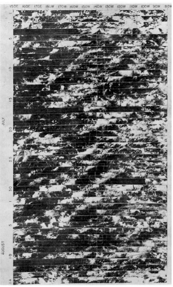
It has long been known that an important part of the synoptic and larger-scale variabilityin the Tropics is due to propagating disturbances moving in the zonal direc- tion. Such disturbances organize individual convective elements on a spatial scale that is larger than the size of the elements themselves. A well-known example are the westward moving synoptic-scale disturbances within the intertropical convergence zones that were visible in time-longitude plots of cloudiness viewed from early satellites (e.g., Fig.1, as taken from Chang 1970). An- other well known example, but on an even larger scale, is the Madden-Julian oscillation, that is often observed as a continental-scale organization of convection mov- ing slowly to the east across the Indian and western Pacic ocean regions. Collectively, all such propagating disturbances are commonly known as `tropical waves', and this paper reviews some of the characteristics of the larger-scale tropical waves known from observations, as well as presenting a technique for diagnosing and fore- casting them in real time.
For this purpose, I rely heavily on the data analy- sis techniques of spectral analysis and ltering. The paper is not intended as a complete review of the scien- tic literature, but instead draws mostly upon my own research and perspective of the current state of knowl- edge. References to theory will mostly be made to the standard text books on atmospheric dynamics only, for example, Gill (1982) and Holton (1992).
2. Spectral analysis
Spectral analysis is used commonly in the study of weather and climate data for identifying any oscilla- tions or dominant scales of variability that may exist.
When spectral analysis is performed on a data series it essentially transforms the series into a set of new quantities that describe the amplitude of each of the
harmonics of the series, that is, it looks at the contribu- tions made at dierent scales. For example, a long time series of hourly temperature data will usually exhibit strong variations both at the daily time scale (corre- sponding to the diurnal cycle of solar heating) and at the annual time scale (reecting the annual solar cycle).
In this paper we are interested in time scales between these extremes, that is, the synoptic to intraseasonal.
a. Frequency spectrum for the Madden-Julian oscilla- tion
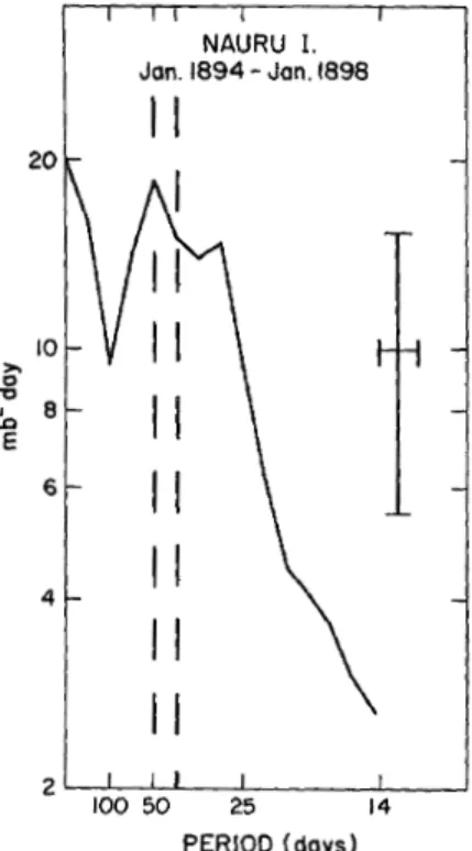
An example of a spectrum of a meteorological quan- tity in the tropics is presented in Fig.2. Shown is the spectral power for pressures recorded at Nauru Island in the late 1800s. Only the power for frequencies cor- responding to a period of 14 days up to a period of 360 days is shown. In general, the power spectrum is quite `red' in character, with the most power (per unit bandwidth) occurring for the lowest frequencies. This is a common characteristic of most geophysical time se- ries, and is especially the case in this time series when one notes that the power is plotted on a logarithmic scale. Besides this `redness', the spectrum also shows a prominent and wide local maximumin the period range of about 30 to 60 days (with an absolute peak at around 40{50 days). This spectral maximum, or `peak', indi- cates that there is an inclination (at least during 1894{
1898) for the pressure at Nauru to oscillate with periods somewhere between 30 and 60 days, and this inclination occurs more often, or with greater amplitude, than for oscillations with periods outside this range (e.g. at pe- riods of 100 days or 14 days).
Tests of statistical signicance may be applied to
power spectra to determine whether a spectral peak
is signicantly dierent from that which could be pro-
duced by noise. In the case of the power spectrum at
Nauru (Fig.2), a comparison to a red noise background
spectrum, that is, one that is continuously increasing
g
Fig.
1:
Time-longitude section of satellite photographs of the period 1 July{14 August 1967 for the 5{10N latitude band in the Pacic. The westward progression of the cloud clusters is indicated by the bands of cloudiness sloping down the page from right to left (taken from Chang 1970).Fig.
2:
Power spectrum for station pressures at Nauru Is- land, 0.4S, 161.0E. Ordinate(varianceper intervalof frequency) is logarithmic and abscissa (frequency) is linear. The 40{50-day period range is indicated by the dashed vertical lines. Prior 95%condencelimits and the bandwidth of the analysis (0.008 day;1) are indicated by the cross (taken from Madden and Julian 1972).
with decreasing frequency (i.e., sloping up to the left), makes the most sense. What actually constitutes the background power spectrum can only be estimated, and in the case of Fig.2, it would be reasonable to estimate it as a straight line sloping down to the right, passing near the local minimum in the spectrum at a period of 100 days, and along the part of the spectrum near a period of around 20 days. The spectral peak between 30 and 60 days would evidently be much above such a background spectrum, and as has been shown by many researchers (the rst being Madden and Julian, 1971 and 1972), such a spectral peak in the data is both sta- tistically signicant (i.e., to a high degree of condence it could not have occurred by chance) and robust (i.e., it appears in the analysis of a number of dierent mete- orological variables, for stations throughout the tropical Indian Ocean to western Pacic regions, and for any pe- riod spanning at least a few years). The phenomenon contributing to this spectral peak is called the Madden- Julian oscillation or MJO. We now know it to be a very important mode of intraseasonal variability in the trop- ics. It is also known to be a propagating disturbance to the east, thus it can be called a tropical wave.
Spectral analysis can also be performed in two dimen- sions. If the input dimensions are longitude and time (e.g., as in Fig.1), the output spectrum is a function of both zonal wavenumber and frequency. Such an analy- sis is quite useful for the study of zonally-propagating waves because it decomposes the longitude-time eld into spectral components separately for eastward and westward propagating waves.
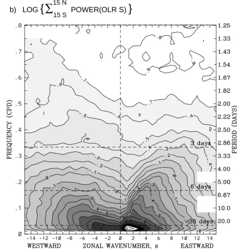
Fig.3 shows a wavenumber-frequency spectral anal- ysis of a long time-series of tropical outgoing long- wave radiation (OLR) data, a good indicator of cloudi- ness and moist convection in the tropics. As I will discuss, these gures form a good summary of the dierent time and space scales of variability acting in the tropics. Prior to calculating the spectra, the data were separated into antisymmetric and symmet- ric components about the equator. They are dened as OLRA(
) = [OLR(
)
;OLR(
;)]
=2 and OLRS(
) = [OLR(
)+OLR(
;)]
=2, respectively, where
is the lat- itude and
;is the latitude on the opposite side of the equator. The original total eld can be reconstructed as OLR(
) = OLRA(
) + OLRS(
). This separation has been done because, as it turns out, many of the tropical waves that can be discerned in the data can be related to the theoretical equatorial waves, and these are either symmetric or antisymmetric about the equa- tor. The power is thus displayed separately for each of these components, summed over the latitudes of 15
S to 15
N. The display in Fig.3 is also such that eastward propagating components are dened to have positive wavenumber (i.e., on the right of each panel), while the westward-propagating components are dened to have negative wavenumber (i.e., on the left).
Looking at the spectra in Fig.3 then, we see that like in Fig.2, the spectra are quite red, but this time in both frequency and wavenumber. That is, the power is concentrated around planetary zonal wavenumber-0 (i.e. the zonal mean) and the lowest frequencies. The absolute spectral peak anywhere in the domain, how- ever, is at around eastward wavenumbers 1 to 2, and periods between 30 and 90 days (the lowest frequency displayed is 1/96 cpd). This spectral peak is for the MJO, the same phenomena that appeared in Fig.2, and it can be seen to be present mostly in the symmetric component, but also somewhat in the antisymmetric component.
Also noticeable in the spectra are several `ridges'
in the contours. For example, in the antisymmetric
component for westward propagating waves with pe-
riods around 4 to 6 days and wavenumbers 0 to
;5.
g
∑
a) LOG
{
POWER(OLR A) 15 N}
15 S b) LOG
{
POWER(OLR S)∑
15 N}
15 S
Fig.
3:
Zonalwavenumber-frequencypowerspectraofthe(a)antisymmetriccomponentand(b)symmetriccomponentofOLR,calculatedfortheperiodofrecordfrom1979to1996usingtwice-dailyobservations.Thepowerwascalculatedindependentlyateachlatitude(ona2.5grid)andthensummedover15Sto15N.Thebase-10logarithmwasappliedfortheconvenienceofplotting.Contourintervalis0.1arbitraryunits.Shadingisincrementedinstepsof0.2.Certainerroneousspectralpeaksfromartifactsofthesatellitesampling(eastwardwavenumber14andperiodsof9and4.5days)arenotplotted.MoredetailsareinWheelerandKiladis(1999).LOG { BACKGROUND SPECTRUM (OLR) }
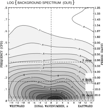
Fig.
4:
Zonal wavenumber-frequency spectrum of the base- 10 logarithm of the \background" power calculated by averaging the individual power spectra of Figs.3a and 3b, and smoothing many times with a 1-2-1 lter in both wavenumber and frequency.The contour interval and shading are the same as in Fig.3 (taken from Wheeler and Kiladis 1999).
These ridges are each an indication that there is more power acting at these scales than for the surrounding scales. In fact, it turns out that many of the ridges are statistically-signicant spectral peaks when compared to a red-noise background spectrum. Such a red-noise background spectrum is displayed in Fig.4, where this spectrum was simply constructed as a smoothed version of the original spectra.
Taking the ratio of the original spectral power (Fig.3) with the background (Fig.4) gives the contours dis- played in Fig.5. With shading, the statistically signif- icant spectral peaks are highlighted, and we now see a variety of spectral peaks which can each be associated with a particular tropical wave.
c. Identifying the tropical waves
Given the spectral peaks of Fig.5, we may identify the following tropical waves.
First, we have the MJO at low eastward-propagating wavenumbers and low frequencies (about 30 to 60 days), as already discussed. Of note here is that its spectral peak is proportionallygreater than the background than any of the others (i.e. its ratio in Fig.5 is generally greater than 2
:0, something that is unfortunately ob-
peak).
Second, we have a number of spectral peaks that can be associated with theoretical equatorial waves. These are the spectral peaks that lie along the theoretical `dis- persion' curves that are also plotted. Ignoring for the moment where such curves come from, we see that they can be used to dene a number of equatorial waves in the observations, and since they imply a coupling be- tween the convection and the dynamics, they are called the \convectively coupled equatorial waves". They are the Kelvin wave,
n= 1 equatorial Rossby (ER) wave, and
n= 1 westward inertio-gravity (WIG) wave in the symmetric component of the OLR, and the mixed Rossby-gravity (MRG) wave,
n= 0 eastward inertio- gravity (EIG) wave, and
n= 2 WIG wave in the an- tisymmetric component. Other theoretical equatorial waves are curiously absent from the spectra, for exam- ple,
n2 equatorial Rossby waves and
n1 EIG waves.
1The MJO, being away from any of the disper- sion curves, is evidently unlike the convectively coupled equatorial waves.
Third, there is an indication of enhanced variance (relative to the background) in both the antisymmetric and symmetric components for synoptic-scale (plane- tary zonal wavenumber,
s6) westward-propagating waves with periods between 3 and 6 days. This region of enhanced variance is associated with the disturbances that are observed within the intertropical convergence zones (ITCZs), and which have been variably called
\easterly waves"
2and \tropical-depression" (TD) -type disturbances. They often exist in the convection on one side of the equator only, hence their appearance in both the antisymmetric and symmetric components. This, together with their variable period and spatial struc- ture from one region to the next, makes them the most dicult of the tropical waves to dene by this spec- tral analysis, as is evident by their diuse, and weak, spectral peak. For this reason, the rest of this paper concentrates less on the classic easterly waves than the
1Note that then= 2 Rossby wave would be antisymmetric in this eld, and then= 3 symmetric. See also Section 5.
2The term \easterly wave" has been used rather loosely in the historical research literature such that almost any large-scale tropicaldisturbanceobservedmoving toward the west (i.e. a wave in the trade-wind easterlies) has at times been given that name, including some of the disturbances that may be better catego- rized as equatorial waves. Most notably, the convectively cou- pled mixed Rossby-gravity waves have often been wrongly iden- tied as easterly waves. I prefer to use the term easterly wave only for those disturbances that have no apparent link with an equatorially-trapped wave. When dened in this manner, the dynamics of easterly waves resembles that of a (non-equatorially- trapped) Rossby wave (e.g. Sobel and Horinouchi 2000).
g
a)
{
POWER(OLR A)∑
15 N}
15 S
/
BACKGROUND b){
POWER(OLR S)∑
15 N}
15 S
/
BACKGROUNDMRG
n=0 EIG n=2 EIG n=2 WIG
n=1 EIG n=1 WIG
Kelvin n=1 ER
50 50
25
12
25 25
50
50 12
12
12 TD-type
25
MJO MJO
TD-type
Fig.
5:
(a)TheantisymmetricOLRpowerofFig.3adividedbythebackgroundpowerofFig.4.Contourintervalis0.1,andshadingbeginsatavalueof1.1forwhichthespectralsignaturesarestatisticallysignicantlyabovethebackgroundatthe95%level(basedon500dof).Superimposedarethedispersioncurvesoftheevenmeridionalmode-numberedequatorialwavesforthethreeequivalentdepthsofh=12,25,and50m.(b)SameasinpanelaexceptforthesymmetriccomponentofOLRofFig.3bandthecorrespondingoddmeridionalmode-numberedequatorialwaves(takenfromWheelerandKiladis1999).a) Regions of filtering for OLR A (Antisymmetric) b) Regions of filtering for OLR S (Symmetric)
MRG
n=0 EIG n=2 WIG
n=1 WIG
Kelvin
n=1 ER MJO MJO
s=0,n=0 IG
Fig.
6:
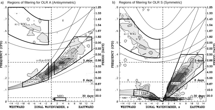
Regions of wavenumber-frequency ltering (thick boxes) used to extract the various tropical waves (excluding `easterly waves') from the OLR dataset for the (a) antisymmetric component and (b) symmetric component of the OLR. The box outlines are drawn such that they are inclusive, meaning that the wavenumber or frequency along which the thick line is drawn is included. Also shown are various equatorial wave dispersion curves for the equivalent depths ofh= 8, 12, 25, 50, and 90 m (taken from Wheeler and Kiladis 1999).other classes of tropical zonally-propagating waves.
3. Diagnostic wavenumber- frequency ltering
The characteristics of the various tropical waves may be studied further through the use of ltering. Filtering is a commonly used diagnostic tool in research as it can extract the variability acting on dierent time and/or space scales from a meteorological dataset. Its use by forecasters, on the other hand, is comparatively rare, the reason being that standard methods of frequency ltering require information for times beyond the time of interest, something that can not be obtained for real- time analysis. In this section we use ltering to look at the characteristics of past events of tropical waves, that is, what I call diagnostic ltering. Examples of ltering applied in a real-time situation will be given later in Section 7.
When ltering one must rst dene the frequencies and/or wavenumbers that one would like to extract.
For the best-dened tropical waves, that is, the ones appearing as strong spectral peaks, we dene the re-
gions as presented as the boxes in Fig.6. Note that the MJO is dened to include both antisymmetric and symmetric components while the convectively coupled equatorial waves are dened to be either in one compo- nent or the other only.
While there are a variety of ways to perform ltering, here we use forward and inverse Fourier transforms, re- taining only those spectral coecients of the boxed re- gions before the inverse transforms. The technique is best shown through examples.
a. Example time-longitude realizations
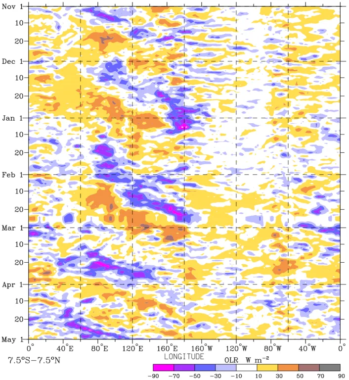
Fig.7 shows a section of unltered daily-averaged OLR for the period November 1987 to April 1988. For the convenience of viewing, anomalies with respect to the mean annual cycle are shown. The blue and purple shades are representative of enhanced convection and rainfall while the orange shading is representative of suppressed. A number of cases of eastward propagating anomalies at various scales can be discerned.
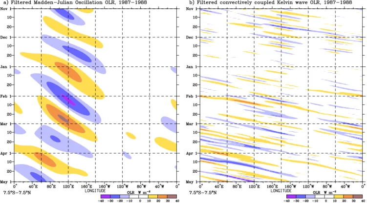
Fig.8 shows ltered elds for the MJO and convec- tively coupled Kelvin wave for the same period as Fig.7.
Comparing the gures, one can identify most of the
g
Fig.
7:
Time-longitude section of daily OLR anomalies averaged for the latitudes from 7.5S to 7.5N. The anomalies are calculated by removing the long-term mean and the rst 3 harmonics of the annual cycle at each grid-point.eastward-propagating anomalies in the unltered eld with either of these two types of tropical waves. The MJO events have a period around 1.5 months and are slowly propagating eastwards, while the Kelvin waves are faster propagating, and with a higher frequency.
Both of these tropical wave types are an important in- uence for the weather in this latitude band during this period. At other times and for other latitudes, how- ever, other tropical waves may dominate. For example,
the o-equatorial section of Fig.1 is likely dominated
mostly by a combination of MRG waves, ER waves,
and easterly (or equivalently TD-type) waves.
Fig.
8:
As in Fig.7 except for sections of (diagnostically) ltered OLR anomalies for (a) the MJO and (b) the convectively coupled Kelvin wave.b. Geographical distributions of the ltered OLR vari- ability
Other characteristics of the tropical waves that may be studied by ltering are their typical locations of oc- currence. Filtering the whole OLR dataset (
20 years worth), one may calculate the standard deviation of each of the ltered elds at each grid-point, and plot it as a map.
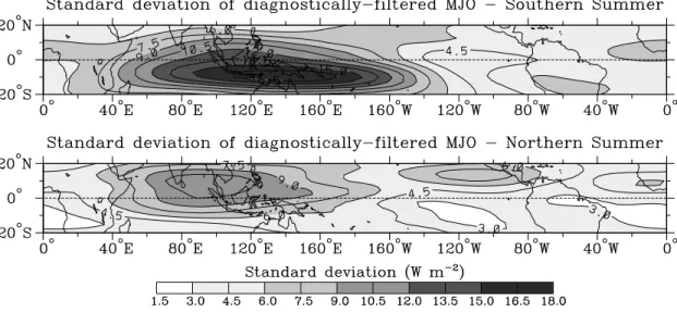
Fig.9 shows such maps for the MJO ltering, sep- arately for southern summer (dened as November through April) and northern summer (May through Oc- tober). In terms of moist convection, for which OLR is a good proxy, the MJO can be seen to be most active around the latitudes of about the equator to 15
S in southern summer, and at latitudes north of the equator in northern summer. Further, the longitudinal extent of the MJO convection can be seen to be restricted mostly to the Indian and western Pacic ocean regions.
Fig.10 displays the same quantity except for the
n
= 1 ER wave. Compared to Fig.9, it is notable that the displayed maps for the ER wave are symmetric about the equator. This is because we dene the ER wave as being in the symmetric component of the OLR (i.e., OLRS) only, as indicated in Fig.6. Also in compar- ison to Fig.9, one can see that the standard deviations for the ER wave are in general less than those for the
MJO, thus the ER waves explain less of the convective
`weather'.
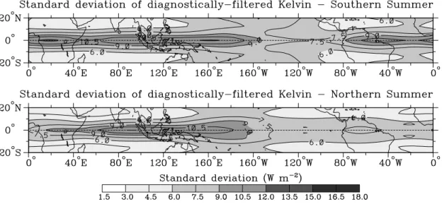
Turning now to the geographical distribution of the standard deviation of the Kelvin wave OLR (Fig.11), we see that it is typically much more concentrated near the equator, and has a more global extent than the other waves, extending even into the Atlantic. Indeed, this distribution of the standard deviation appears quite consistent with the snapshot of the total record provided in Fig.8b.
Further, the geographical distribution of the MRG wave variability is displayed in Fig.12. This tropical wave is most active during northern fall, so we display its standard deviation for this portion of the year only.
Of note is that this type of wave tends to be most active in a region around the date line, yet it can be observed almost anywhere across the Indian and Pacic ocean sectors as well, inuencing convection primarily at o- equatorial latitudes from about 5 to 10
.
4. `Conceptual models'
A conceptual model of a meteorological phenomenon
is dened as an attempt to specify the idealized or gen-
eralized space distribution of meteorological elements
g
Fig.
9:
Standard deviation of the diagnostically-ltered MJO OLR for the 10-year period of 1985 to 1994, separately for southern summer (above) and northern summer (below) (taken from Wheeler and Weickmann 2001).Fig.
10:
As in Fig.9 except for the convectively coupledn= 1 equatorial Rossby (ER) wave (taken from Wheeler and Weickmann 2001).such as clouds, rainfall, wind, temperature or pressure in that distinct type of atmospheric system. Here we briey look at some of the conceptual models that have been produced for the lower-frequency tropical waves.
Often, spectral analysis and ltering of the historical datasets is used in the process of producing such con- ceptual models.
a. Madden-Julian oscillation
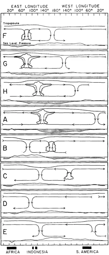
This is the most well-known of the tropical waves, and its most well known conceptual model is repro- duced in Fig.13. This gure is a schematic based on the evidenced amassed by Madden and Julian from com-
positing a number of MJO events during an 18-month period (during 1957{1958). It gives an indication of the vertical structure of the wave along the equator.
Of note is the fact that the schematic indicates that
the convection associated with the MJO is limited to
the Indian to western Pacic Ocean regions, while the
(anomalous) circulation associated with the MJO has
a more global extent. Over the Indian to western Pa-
cic sectors the circulation is `coupled' to the convec-
tion, while elsewhere the circulation is essentially `dry',
that is, without convection. Also, the dry vertical cir-
culation component over the central to eastern Pacic
propagates more quickly to the east than the convective
component over the warmer waters of the western Pa-
Fig.
11:
As in Fig.9 except for the convectively coupled Kelvin wave (taken from Wheeler and Weickmann 2001).Fig.
12:
As in Fig.9 except for the convectively coupled mixed Rossby-gravity (MRG) wave, and for the season of northern fall (dened as August to January) only (taken from Wheeler and Weickmann 2001).cic. The speed of propagation of the latter is about 5 m s
;1, consistent with that obtained from the ltering of OLR for a sequence of cases in Fig.8a.
What the schematic of Fig.13 doesn't show about the MJO, however, is its typical horizontal structure.
A useful conceptual model of this is as presented in the schematic of upper-tropospheric circulation for the MJO in Fig.14. This schematic was constructed based on spectral and cross-spectral analysis of many years of data. An important feature of this circulation is that it has the appearance of what is commonly known as the Gill pattern, after Gill (1980), with o-equatorial cir- culation cells of a forced equatorial Rossby wave to the west of the \cloud" region and equatorial zonal ow of a Kelvin wave to the east.
3Of course, to identify such circulation patterns in an operational forecaster's syn- optic chart would be quite dicult, as not only would this pattern of ow be superimposed upon the mean winds (e.g. those of the mean Walker and Hadley circu-
3For a brief discussion of the essential theoretical characteris- tics of equatorial Kelvin and Rossby waves, refer to Section 5.
lation cells), but it would be superimposed upon vari- ability acting on other time scales as well (e.g. tropical cyclones and other tropical waves).
b. Convectively coupled
n= 1 equatorial Rossby wave
A conceptual model of a convectively coupled
n= 1
ER wave is provided in Fig.15. Shown are horizon-
tal maps of anomalous OLR, 850 hPa streamfunction,
and 850 hPa winds calculated from observations using
a regression technique. The regressions were computed
at various lags against an index of the ER waves con-
structed by ltering. This `typical' convectively coupled
ER wave can be seen to consist of anomalous circula-
tion cells on both sides of the equator slowly moving to
the west with new circulation cells developing to their
east. The propagation (phase) speed of these features
is around 5 m s
;1to the west. The negative anoma-
lous OLR, and hence enhanced convection, tends to be
in the regions of anomalous low-level poleward and/or
westerly ow. Such a structure for the ER wave is usu-
g
Fig.
13:
Schematic depiction of the time and space (zonal plane) variations of the Madden-Julian oscillation. Dates are indicated symbolicallyby the letters at the left of each chart and each panel is separatedby approximately5{6 days. The pressure of the disturbance is plotted at the bottom of each chart with negativeanomalies shaded. The circulationcells are based on the zonal winds, with the vertical motion coming from what may be inferred from continuity considerations and observations of humidity. Inferred regions of enhanced large-scale convection are sketched as clouds. The relative tropopause height is indicated at the top of each chart (taken from Madden and Julian 1972).Fig.
14:
Schematic of the relationship between convection, as signied by \cloud" and \clear" regions, and the 250-hPa circulation for the MJO at a time when maximum cloudiness is over the Indonesian region (taken from Weickmann et al. 1985).ally best developed in the mid to lower-troposphere.
c. Convectively coupled Kelvin wave
Fig.16 presents the typical horizontal structure of a convectively coupled Kelvin wave, as also calcu- lated from regression analysis. It shows the upper- tropospheric ow and geopotential associated with the wave, together with the OLR. Like for the MJO, the region of enhanced convection propagates to the east with the wave, although at a much faster rate (about 15 m s
;1). The convection is also more concentrated at the equator than what is observed for the MJO, with a smaller meridionalextent. The ow is also mostly zonal, without the Rossby gyres of the Gill-pattern of the MJO (cf. Fig.14). Evidently, this is another distinct mode of the tropical atmosphere that deserves its own con- ceptual model. In some of the research literature it has been called a \supercluster" or \super cloud cluster".
Further, like all of the tropical waves it may occur ei- ther in conjunction with other waves or independently.
Only during times when it is acting independently is it likely to be seen in a standard synoptic analysis chart as typical wind anomalies are only on the order of 2 m s
;1.
d. Convectively coupled mixed Rossby-gravity wave Another useful conceptual model is provided in Fig.17. It presents the typical lower-tropospheric struc- ture of a convectively coupled MRG wave. Like in the
conceptual model gures for the other tropical waves, this plot shows anomaly elds only. In the anomalies, the MRG wave presents itself as circulation cells centred on the equator (moving to the west) with enhanced con- vection mostly in regions of low-level poleward ow. If one was to superimpose the anomaly elds upon the mean easterlies that occur in this region, however, the result would look somewhat dierent. Instead of dis- tinct circulation cells, the strength of the mean winds may be such that the wave appears as a north-south me- andering in the easterly streamlines only. Importantly, such meandering streamlines, or `troughs' and `ridges' in the easterlies, are predominantly antisymmetric across the equator for the MRG wave. This is the primary distinction between this wave and what is best dened as an easterly wave, as shown next.
e. Easterly waves or tropical depression-type distur- bances
The horizontal structure of a typical easterly wave of the northwestern Pacic is shown in Fig.18. As has already been mentioned, this wave typically shows per- turbations on one side of the equator only. It also has quite a strong signature in the vorticity eld. As such, it has been found by researchers that many aspects of their dynamics can be explained by barotropic Rossby wave theory, that is, non-equatorially-trapped Rossby waves.
Enhanced convection is typically in the region of the cy-
clonic vorticity and/or poleward ow. If a trough axis
was drawn, this region of enhanced convection would
g
Fig.
15:
Typical horizontal structure of anomalies associated with a convectively coupledn= 1 equatorial Rossby wave over a sequence spanning 21 days, as calculated using regression analysis. Shading/cross-hatching show the negative/positive OLR anomalies, indicating enhanced/suppressed convection. Contours are streamfunction anomalies at the 850 hPa level, indicating the lower-level rotational winds. Vectors are the 850-hPa wind anomalies of the wave (taken from Wheeler et al. 2000).be near and to the east of the trough axis. Although dicult to consistently dene, they appear to be com- mon in both the Pacic and Atlantic regions, generally north of the equator. Like the MRG and ER waves, they propagate to the west.
5. Some discussion of theory
As can be discerned from the preceding discussion, many of the features of the tropical waves can be well
described and understood by some rather simple theory, that is, the theory of equatorially-trapped waves. It is thus useful to have some understanding of this theory.
Here, I will mostly describe the concepts of the theory in words. For a more complete development refer to sections 11.4 of the texts of Gill (1982) or Holton (1992).
The theory may start with what are known as the
primitive equations, that is, the full set of basic equa-
tions that governs the time evolution of the three-
dimensional large-scale motion eld in the (dry) strat-
ied atmosphere. These equations are often written as
Fig.
16:
Typical horizontal structure of anomalies associated with a convectively coupled Kelvin wave over a sequence span- ning 9 days, as calculated using regression analysis. Shading/cross-hatching show the negative/positive OLR anomalies, indicating enhanced/suppressed convection. Contours are geopotential height anomalies at the 200 hPa level. Vectors are the 200-hPa wind anomalies of the wave (taken from Wheeler et al. 2000).a) MRG at 850 hPa [OLR, ψ, (u,v)]
Fig.
17:
Typical horizontal structure of anomalies associated with a convectively coupled mixed Rossby-gravity wave, as calculated using regression analysis. The same elds are shown as in Fig.15.six equations in six unknowns: the zonal velocity, merid- ional velocity, vertical velocity, density, pressure, and temperature.
The full primitive equations are no doubt dicult to analyse. However, given certain assumptions (e.g. lin- earized equations about a basic state with no motion), the primitive equations may be separated into an in- nite set of independent \shallow water" equations, and a vertical structure equation. The shallow water equa-
tions govern the horizontal and time-varying behaviour of the ow of each \normal mode", and are written as three equations in three unknowns only. They are evi- dently much simpler to analyse, and can be written for the equatorial region as
@u 0
l
@t
;y v 0
l
=
;@0l@x
(1)
@v 0
l
@t
+
y u0l=
;@0l@y
(2)
g
Fig.
18:
Typical horizontalstructureof anomaliesassociatedwith an \easterlywave" or \tropical-depression"(TD) -typedisturbance in the northwest Pacic, as calculated using regression analysis. Shown are 850-hPa winds (m s;1) and 850-hPa vorticity (10;5 s;1) (taken from Sobel and Bretherton 1999).@
0l@t
+
g hl@u0l@x
+
@v0l@y
= 0 (3)
where
is the equatorial value of the
-parameter (
@f=@y),
gis the acceleration due to gravity,
hlis the equivalent depth,
u0land
v0lare the (horizontal) velocities in the
xand
ydirections respectively, and
0lis the geopotential. Of note is that we have applied what is known as the equatorial
-plane approximation here, where the Coriolis parameter
fis replaced by the linear function
y, where
is assumed to be constant.
Further, the primes denote the fact that these are per- turbation elds relative to the basic state of no motion about which the equations are linearized, while the
lsig- nies that these equations govern a particular vertical normal mode only. In the shallow water equations, the unknown variables are a function of horizontal position (
x;y) and time (
t) only.
Note that although these equations as written are equivalent to those for perturbations to the free sur- face of a shallow layer of incompressible, homogeneous density uid of mean depth
hl(also called the divergent barotropic model), these equations are equally valid for internal modes of motion of the stratied atmosphere provided the correct choice of
hlis made. Then, the full three-dimensional structure of the internal modes of motion is obtained by multiplying the shallow water solutions by an appropriate vertical structure function, that is, a function of height (
z).
Without going into the details of the mathemati- cal analysis, it is sucient for this paper to say that
the \equatorial waves" are the valid wave-solutions of the shallow-water equations (1){(3) in the vicinity of the equator. Everything that is needed to dene their rather complicated structure and properties is included in these equations, and these characteristics can be neatly described by what are known as the dispersion re- lations of the waves (Fig.19), and their horizontal struc- tures (e.g., Fig.20). Their existence relies crucially on the change in sign of the Coriolis force at the equator, as is contained in the term
y.
Looking at Fig.19, we see the same curves that were used to dene some of the tropical waves in Fig.5.
There are two main classes of waves, along with two additional waves. The two classes are the Rossby (or planetary) waves, which are westward propagating only, and the inertio-gravity waves, which can be either west- ward or eastward. Individual waves within these classes are denoted by a dierent integer value of
n, where
nis the meridional mode number. Waves of larger
nhave more complicated meridional structures. The two ad- ditional waves are the mixed Rossby-gravity wave and the Kelvin wave. The higher frequency waves tend to be more divergent in character, while the lower frequency waves are more rotational (and geostrophic).
The curves in Fig.19 are drawn as functions of non- dimensionalized frequency and wavenumber. When drawn for dimensionalized units (as in Fig.5), an impor- tant parameter for their value is the equivalent depth,
h
l
. For large-scale internal modes of motion in the tro-
posphere, realistic equivalent depths may be anywhere
Fig.
19:
Dispersion curves for equatorial waves (up to n= 4) as a function of the non-dimensional frequency, , and zonal wavenumber,k, where=(pg hl)1=2, andkk(pg hl=)1=2(as in Matsuno 1966). These dispersion relations ultimately come from the shallow water equations, (1){(3). Eastward propagating waves (relative to the zero basic state employed) appear on the right, and westward propagating waves on the left.in the range of about 10 to 300 m. As is indicated in Fig.5, the convectively coupled equatorial waves occupy the lower end of this range. Equatorial waves that are not coupled to convection may exist for higher equiva- lent depths (
200 m). This serves to cause the convec- tively coupled waves to exist for lower frequencies than
`dry' waves of the same wavenumber. Equivalently, the convectively coupled waves move more slowly than the dry waves.
Another useful concept from the theory is that of phase speed and group velocity. Noting that the zonal phase speed is dened as
cp =k, and the group velocity as
cg @=@k(see, for example, section 7.2 of Holton 1992), the dierent dispersion characteristics may be inferred from the curves of Fig.19. That is, the group velocity is the local slope of the curves, while the phase speed is determined by the position on the diagram relative to the origin.
The group velocity determines how the energy of a
`packet' of each of the waves will disperse. Thus for a Kelvin wave, for which
/ k, the group velocity is identical to the phase speed, and thus the wave is non- dispersive. This is consistent with the observations of Fig.16 for which the energy and the phase propagate
together to the east. Conversely, the group velocity of an equatorial Rossby wave is near zero (the dispersion curves have near zero slope) hence the energy of the wave packet in Fig.15 stays in much the same place, while an individual component (or phase) of the wave propagates through the wave packet to the west.
Fig.20 displays horizontal structures for four of the more common equatorial waves. Many further con- sistencies can be seen between the theoretical waves and the observed convectively coupled equatorial waves.
The MRG wave has circulation cells centred on the equator while the
n= 1 ER wave consists of twin cir- culation cells on both sides of the equator. The Kelvin wave, on the other hand, consists of purely zonal ow.
The regions of divergence and convergence of the theo- retical waves, as indicated by shading, are also generally consistent with the regions of suppressed and enhanced convection of the observed equatorial waves, with the
n
= 0 waves being antisymmetric, and the
n= 1 ER
and Kelvin waves symmetric. In contrast, the easterly
waves (Fig.18) have horizontal structures that do not
easily match any of the equatorial waves, while the MJO
(Fig.14) has a structure that combines components of
both the Kelvin and
n= 1 ER waves.
g
a) b)
c) d)
Fig.
20:
Horizontal structures of the (a) mixed Rossby-gravity wave, (b)n= 0 eastward inertio-gravity wave, (c) n= 1 equa- torial Rossby wave, and (d) Kelvin wave, each for non-dimensional zonal wavenumberjkj= 1. All scales and elds have been non- dimensionalized by taking the units of time and length as [T] = (1=pg hl)1=2, and [L] = (pg hl=)1=2, respectively. The equator runs through the center of each diagram. Hatching is for convergence and shading for divergence, with a 0.6 unit interval between successive levels. Unshaded contours are for geopotential, with a contour interval of 0.5 units. Negative contours are dashed and the zero contour is omitted. The largest wind vectors are as specied in the bottom-right corner.Finally, the above theory is strictly for dry waves, those without the inuence of convection, only. For the observed tropical waves, interaction between the con- vection and dynamics is no doubt important, after-all, the latent heating of convection is one of the most im- portant energy sources for atmospheric motions in the tropics. While many theories have been developed to attempt to account for such interaction, they are not as well accepted as that for the dry waves. In general,
however, the theories all usually result with the con- clusion that the moist, convectively coupled waves slow down relative to their dry counterparts.
6. Some discussion of forecasting
So far, this paper has concentrated on showing just
the existence and characteristics of the tropical waves.
casting has not yet been discussed.
It is rst of note that each of the tropical waves ex- plain only a fraction of the total variability of the con- vective weather. Even the MJO, which on the whole explains the most variance (Fig.9), accounts for only on the order of 10% of the total OLR variance of all scales from diurnal up to seasonal on a 2.5
grid. Of course, the MJO would explain a greater portion of the variance of 5-day means, and a greater portion of the variance of a larger-scale average (e.g. a 10
latitude by 10
longitude average). Thus if forecasts of say the 5- day mean precipitation over a 10
box are considered to be useful, then predictions of the MJO would certainly be useful.
Despite their `explanation' of less of the overall vari- ance, benet may also come from forecasts of the other tropical waves, especially considering that at times they are quite strong. For example, the convectively coupled Kelvin waves of Fig.8b are noticeably stronger in the eastern hemisphere during March and April than dur- ing the preceding months. During times that a particu- lar tropical wave disturbance is strong, it accounts for a greater portion of the total variance, and at these times certain benet could come from forecasting them.
Also of note is that many of the various tropical waves have time scales that are quite relevant to atmo- spheric prediction, especially on the medium to longer range (i.e., greater than a few days, see Fig.5), and this time scale is currently at or beyond the limit which can be skillfully forecast by numerical weather prediction (NWP) models in the tropics, especially with regards to convection or rainfall. An example of NWP forecasts of tropical precipitation in Fig.21 illustrates this.
The far left panel of Fig.21 shows precipitation rates derived from the satellite-borne microwave sounding units (MSU) for the period December 1987 through April 1988 averaged from 15
S to the equator. Three prominent enhanced convective phases of the MJO can be seen propagating to the east across the domain. The MJO has a fairly consistent period of about 1.5 months during this time.
The middle and right panels of Fig.21 show how well this precipitation could have been forecast by a fairly modern (as of 1996) NWP model, specically, the U.S. National Center for Environmental Prediction (NCEP) T62L28 Medium Range Forecast (MRF) model (Schemm et al. 1996). The 5-day forecasts show some evidence of the intraseasonal MJO variability, but the 15-day forecasts show no evidence of the variability at all. Clearly, a subjective forecast based on the knowl- edge of the existence of the MJO could have provided
or empirical predictions of the MJO and other longer time-scale tropical waves can provide a better medium to longer-range forecast than a NWP model. The next section presents such an empirical forecasting technique.
7. Real time wavenumber- frequency ltering
One of the major diculties for using the large-scale tropical waves for forecasting is being able to identify their existence and location in real time. Unlike what can be done in diagnostic studies of tropical waves (e.g., Section 3), standard methods of low- or band-pass fre- quency ltering cannot be performed, as there is no information beyond the current time, something that is usually required for such ltering. In this section I present a technique for monitoring and predicting the various tropical waves by a method of \real-time" lter- ing. It can be considered to be a form of one-sided lter- ing. For prediction of OLR anomalies, it demonstrates good skill for the MJO, and detectable (although possi- bly not very useful) skill for some of the other tropical waves. For the MJO, the technique compliments other methods of empirical prediction that have also been re- cently developed, in particular, those of Lo and Hendon (2000) and Waliser et al. (1999). Further, although the technique may not necessarily be better than what can be performed by subjective decisions of a human that is skilled at monitoring and predicting tropical in- traseasonal variability, it is something that can easily be automated and used in hindcast experiments for ex- amining the utility of such forecasts in a quantitative manner.
The method of the technique is to take the most re- cent year of OLR data at all longitudes, create anoma- lies with respect to the annual cycle (as calculated us- ing the past 10 years), pad the end of the dataset with zeroes, and perform the wavenumber-frequency ltering with forward and inverse fast Fourier transforms (FFTs) independently at each latitude. No tapering is applied at the end of the dataset before the ltering, thus the ltered elds retain their amplitude up to the end-point.
It is the part of the ltered elds that lead up to the end-point time that we call the real-time monitoring.
The ltered elds that are returned from the FFT pro- cedure for times beyond the end-point of the dataset (i.e., in the zero-padding) are used for the predictions.
More details of the technique are provided in Wheeler
and Weickmann (2001).
g
Fig.
21:
(d) Time-longitude plot of (observed) MSU precipitation. Missing data is left blank and land areas hatched. A 1-2-1 lter has been applied in both space and time for smoothing purposes. (e) As in (d) except for 5-day forecasts of precipitation from the NCEP MRF model verifying on the days as labeled. (f) as in (e) except for the 15-day forecasts. (taken from Wheeler and Weickmann 2001).Fig.
22:
Schematic of the procedureof real-time ltering for monitoringand prediction, as applied to a time series with an MJO-like signal. Note that in the actual procedure, two dimensions of information are used (taken from Wheeler and Weickmann 2001).Fig.22 presents a schematic of the procedure, as ap- plied to the monitoring and prediction of a MJO-like signal. In this schematic, which shows the OLR data to be ltered at a single latitude/longitude location only, notice how the presence of a strong MJO-like signal near the end of the actual data continues as a signal in the ltered time series beyond the end-point of the dataset (i.e., into the zone that was padded with ze- roes). Of course, this ltered signal is inuenced by the presence or absence of a MJO-like signal at other longi- tudes as well. The end-point of the dataset is referred to as Day 0. In an operational setting, Day 0 would be the most recent 24-hour period in UTC time. The pre- dicted OLR anomalies are with respect to the seasonal cycle and any variabilityacting on longer time scales. In this schematic, they can be seen to decay towards zero rather rapidly beyond day 0. Such decay is a general property of all such forecasts, something that a user must keep in mind. Further, although the schematic shows the forecast for a single mode of variability only, the real-time ltering procedure may eciently produce a signal for each of the modes of variability labeled in Fig.6.
An example of the technique applied to actual OLR data around the time of the onset of the Australian monsoon in late 1996 is provided in Fig.23. The left- hand panel shows the total OLR eld along with the diagnostically-ltered anomalies of the MJO and
n= 1 ER waves. This ltering was performed using the entire dataset (i.e. up until 1999). The right-hand panel, on the other hand, shows the real-time ltering that was produced with the end-point of the dataset at the 5th of
December. In this presentation, the predictions are the ltered elds (i.e. the contours) that are presented for times beyond the 5th of December. Note that the con- tour interval used to plot the predicted anomalies has been halved relative to that used to plot the anomalies before Day 0, due to the known decaying property of the predictions by the technique.
Looking at the right panel, we see that the real-time ltering (as could have been produced on the 6th of De- cember) is indicating that there is an enhanced phase of the MJO (solid contours) around 100
E, and it pre- dicts that it should continue to propagate to the east. It also predicts an enhanced phase of the ER wave coming through at the same time. The technique also predicts that there should be suppressed convection associated with the MJO around 60
E from about the 10th to 20th of December. Now comparing this to what actually oc- curred (in the left panel), we see that in this case the real-time ltering performed quite well at providing a forecast of the future evolution of the OLR eld for about 10 or more days ahead.
Showing the success of a single forecast, however, is
not sucient to verify a forecast technique. For this,
many forecasts (or hindcasts) need to be made, and
statistics need to be computed to indicate the true skill
of the technique. Fig.24 shows such a statistic for hind-
casts of the MJO OLR that were computed for a 10-year
period. The statistic shown is the anomaly correlation
at each grid-point between the real-time ltered MJO
OLR, and the diagnostically-ltered OLR (as calculated
using the ltering without nearby end-points). The g-
ure shows that during Southern summer the best fore-
g
Fig.
23:
(a) Time-longitude plot of the total OLR (with R21 spatial truncation, and a 1-2-1 lter applied in time) and ltered OLR anomalies averaged between 10S and 5N during late 1996 to early 1997. Shading is for the total OLR, and contours are for the diagnostically-ltered anomalies of the MJO andn= 1 equatorial Rossby (ER) wave. Solid contours represent negative OLR anomalies, while dashed contours are for positive anomalies, with the contour interval for both wave ltered bands being 10 W m;2, and the zero contour omitted. (b) Same as (a), except that the ltering was performed with the last day of data being on December 5th, 1996. After December 5th, when the real-time ltered anomalies are continued into the future as a forecast, the contour interval is halved (taken from Wheeler and Weickmann 2001).casts of the MJO are made in a region encompassing parts of northern Australia, Papua New Guinea, and across the southwest Pacic centred at a latitude of about 10
S. The correlations for the 15-day forecasts in these regions are greater than 0.6. For the opposite season, on the other hand, the best forecasts are made over the Indian ocean and northeastern Pacic. These correlations seem quite promising, although it must be remembered that they are only indicative of how much of the MJO portion of the variability that is being `ex- plained' by the predictions. When the correlations are computed against a eld containing the total synoptic to intraseasonal variability of OLR, they are notably less, with peak values for a 15-day forecast around 0.3.
Finally, it is of note that the above statistics are cal-
culated during all years, and for the whole season. Yet it is known that the MJO, like other tropical waves, is not always occurring. Thus the statistics may be improved if calculated only for times when the MJO is determined to be relatively strong. It can be similarly shown that at times when one of the other tropical waves is par- ticularly strong, empirical predictions of its phase by this real time ltering technique can also outperform a NWP prediction of precipitation.
8. Conclusion
A variety of well dened `synoptic to intraseasonal'
tropical waves exist in the tropical atmosphere. How-
ever, with the multitude of phenomena occurring at any
Fig.
24:
Correlations of the MJO real-time ltered OLR with the validating diagnostically-ltered MJO OLR for southern summer (upper panels) and Northern summer (lower panels), for a number of lead times in days. Lead time is with respect to the end-point of the data input into the real-time ltering procedure as indicated in the lower left of each panel. All 10 years of the sample forecasts were used (taken from Wheeler and Weickmann 2001).one time in the tropical atmosphere (e.g., numerous tropical waves, tropical cyclones, cold surges, monsoons, island convection etc.) it may be dicult to identify them in a standard synoptic analysis chart showing to- tal elds only. Methods of real-time ltering may be
one way around this. For the MJO, real-time lter-
ing of OLR has already been implemented in a semi-
operational setting, and has shown some success for
both monitoring and forecasting beyond the medium
range (i.e. beyond several days). Until NWP mod-
g