Reinterpretation of searches for supersymmetry in models with variable R-parity-violating coupling

A TLAS-CONF-2018-003 18/04/2018

ATLAS CONF Note

ATLAS-CONF-2018-003

April 18, 2018

Reinterpretation of searches for supersymmetry in models with variable R-parity-violating coupling

strength and long-lived R-hadrons

The ATLAS Collaboration

A selection of ATLAS searches for supersymmetry (SUSY), optimized for R -parity- conserving and R -parity-violating (RPV) models, are reinterpreted in SUSY models with variable RPV-coupling strength. Depending on the coupling strength the lightest supersym- metric particle is stable at collider scales, is long-lived and decays away from the interaction point, or decays promptly. Limits are placed on simplified models of pair-produced gluinos decaying to final states enhanced or depleted with top quarks, and models of pair-produced top squarks. In a model of pair-produced gluinos decaying to final states enhanced with top quarks, a lower limit of 1.8 TeV on the gluino mass is set at 95% confidence level regardless of the RPV coupling value. Limits are set on models of gluino pair production decaying to light- flavor quarks, and models of top squark production. Limits are also placed on meta-stable gluinos decaying within the detector volume.

13

April 2018: after the first release of the result two small errors were identified and corrected, one in the di-nucleon decay limit formula and the other in the λ

323

value in Appendix B. An additional note was added to the stop model discussion on excluded production modes.

© 2018 CERN for the benefit of the ATLAS Collaboration.

Reproduction of this article or parts of it is allowed as specified in the CC-BY-4.0 license.

1 Introduction

Supersymmetry (SUSY) [1–9], is a generalization of space-time symmetries which extends the Standard Model (SM) by introducing supersymmetric partners for every SM particle with identical quantum numbers except for a half-unit difference in spin. The scalar partners of the left- and right-handed quarks, the squarks q ˜

and ˜ q

, mix to form two mass eigenstates ˜ q

and ˜ q

ordered by increasing mass. Superpartners of the charged and neutral electroweak and Higgs bosons, so called winos, bino and higgsinos, also mix producing charginos ( ˜ χ

1,2

) and neutralinos ( ˜ χ

1,2,3,4

) with subscripts indicating increasing mass. Squarks and the fermionic partners of the gluons, the gluinos ( ˜ g), could be produced in strong-interaction processes at the Large Hadron Collider (LHC) with large cross-sections.

In the most generic superpotential, the following Yukawa and bilinear couplings can lead to baryon- and lepton-number violation:

W

= λ

2

L

L

E ¯

+ λ

L

Q

D ¯

+ λ

2

U ¯

D ¯

D ¯

+ κ

L

H

, (1) where i , j , and k are quark and lepton generation indices. The L

and Q

represent the lepton and quark SU(2)

doublet superfields and H

the Higgs superfield that couples to up-type quarks. The ¯ E

, ¯ D

and ¯ U

are the lepton, down-type quark and up-type quark SU(2)

singlet superfields, respectively. The couplings are λ , λ

, λ

, as well as κ which is a dimensional mass parameter. The λ and λ

couplings are antisymmetric under the exchange of i → j and j → k , respectively. While these terms are removed in many scenarios by imposing an additional Z

symmetry ( R -parity) [10], the possibility that at least some of these R -parity-violating (RPV) couplings are not zero is not ruled out experimentally [11, 12].

In this note the lightest neutralino, ˜ χ

1

, is assumed to be the lightest supersymmetric particle (LSP). If R -parity is conserved, SUSY particles are produced in pairs and decay either directly or via cascades to the LSP which is stable and escapes the detector unseen. Introducing non-zero RPV couplings renders the LSP unstable and allows decays to SM particles via the interactions in Eq. (1). The LSP lifetime, τ

, depends on the RPV coupling strength as well as the masses of the sfermions involved in the decay.

Most searches for RPV SUSY assume values of the coupling that are large enough to ensure prompt decays of the LSP. However, in the parameter space of small RPV couplings and/or large sfermion masses the LSP can become long-lived and decay after traversing a sizable distance within the detector volume.

In the limit where the RPV coupling is vanishingly small the majority of LSP decays occur outside the detector volume, producing the same experimental signature as R -parity-conserving (RPC) SUSY. For high values of the coupling, the LSP decays promptly; as the coupling increases even further, squarks and gluinos can decay directly to SM particles via the large RPV coupling. Thus, scaling the value of the RPV coupling transitions the SUSY final state through several distinct regimes. Furthermore, non-zero RPV coupling values allow for single sparticle production. Different ATLAS analyses, described in Section 3, are optimized for different points of this phase space, but a complete analysis of the transition in sensitivity as a function of the coupling strength has never been performed.

Final states with displaced decays can also emerge from models such as Split SUSY [13, 14], where large

mass hierarchies allow bound states involving SUSY particles (called R -hadrons) to obtain macroscopic

lifetimes. Many existing ATLAS analyses target such models explicitly by searching for displaced

vertices [15], anomalous dE/dX in silicon detectors [16], stable charged particle signatures [17], or

decays in empty LHC bunch-crossings [18]. However, depending on the lifetime of these particles, SUSY

searches targeting traditional simplified models can also provide sensitivity to these signatures.

This note presents a reinterpretation of published ATLAS SUSY searches, originally designed for scenarios with either RPC or RPV with prompt LSP decays, in models with baryon-number-violating RPV with variable coupling strength λ

, and in models with variable R -hadron lifetime.

2 SUSY models

The main characteristics of the SUSY models considered in this note are given in Table 1 and detailed in this section.

Model name Gqq Gtt Stop R -hadron

Coupling λ

112

λ

323

λ

323

–

Decay

g ˜ → qq χ ˜

1

g ˜ → tt χ ˜

1

t ˜

→ t χ ˜

1

g ˜ → qq χ ˜

˜

g → qq χ ˜

1

(→ qqq) g ˜ → tt χ ˜

1

(→ tbs) t ˜

→ t χ ˜

1

(→ tbs) g ˜ → qqq g ˜ → tbs t ˜

→ bs Other colored

sparticle masses

m( q) ˜ = 3 TeV m( q) ˜ = 5 TeV m( q, ˜ g) ˜ = 3 TeV

m( q, ˜ t, ˜ b) ˜ ≈ PeV m(˜ t, b) ˜ = 5 TeV m( t, ˜ b) ˜ = 2 . 4 TeV m( t ˜

, b) ˜ = 3 TeV

LSP The LSP is bino-like, m( χ ˜

1

) = 200 GeV m( χ ˜

1

) = 100 GeV Table 1: Summary of signal models. First and second generation squark masses are assumed to be degenerate ( ˜ q = ˜ u , ˜ d , ˜ s , ˜ c ). Left- and right-handed superpartner masses are also assumed to be degenerate ( ˜ q = q ˜

, q ˜

), except for the stop model where the right-handed top quark partner is assumed to be lighter.

2.1 RPV models

The sensitivity of a suite of ATLAS searches is evaluated on a set of simplified SUSY models [19–21].

All models assume the existence of a non-zero baryon-number-violating RPV λ

coupling. Lepton- number-violating couplings, λ and λ

, are assumed to be zero. Within the set of λ

couplings, only one is considered to be non-zero in each simplified model, while the rest are assumed to be zero.1 The antisymmetry condition λ

= −λ

is respected, and is always implied when a model is described as having only one non-zero coupling. Supersymmetric scenarios featuring only baryon-number-violating RPV couplings are predicted in minimal flavor violation (MFV) SUSY [22]. The LSP is assumed to be the lightest neutralino, ˜ χ

1

, which is purely bino-like and has a fixed mass of 200 GeV. The value of the mass is chosen to allow decays of the neutralino to a top quark. The choice of a bino-like neutralino is made for simplicity as the absence of a chargino in the particle spectrum reduces the number of possible squark or gluino decays. The nature of the neutralino has also an impact on its lifetime, e.g. a higgsino-like neutralino has a shorter lifetime due to the large Yukawa coupling to the stop.

1

The absence of lepton-number-violating couplings is enough to satisfy proton stability bounds. The choice of having only one

non-zero baryonic coupling is made for simplicity and the availability of a theoretical upper limit.

Despite the usage of simplified models, the masses of all the squarks have to be specified even if they are not considered in the accessible sparticle spectrum, since the LSP lifetime depends on the choice of squark masses. The results are presented as a function of the RPV coupling strength, λ

, and as a function of the LSP lifetime and branching ratio. The correspondence between coupling strength and lifetime or branching ratio is determined by the choice of squark masses. The mean decay length for a bino-like lightest neutralino can be numerically estimated [23] from:

L(cm) = 0 . 9 βγ λ

m( q) ˜ 100 GeV

!

* ,

1 GeV m( χ ˜

1

) + -

5

(2)

For a fixed value of the coupling higher squark masses lead to higher neutralino lifetimes. The computation of lifetime and branching ratios is performed with SPheno 4.0.2 [24, 25] in combination with SARAH 4.12.0 [26].

˜ g

˜ g p p

˜ χ⁰₁ q

q

˜ χ⁰₁

q q

˜ g

˜ g

˜ χ

˜ χ

p

p

q q

λ

q

q q

q q

λ

q

q q

˜ g

˜ g p

p

λ

q

q q

λ

q q q

˜ g

˜ g p p

˜ χ⁰₁ t

t

˜ χ⁰₁

t t

˜ g

˜ g

˜ χ

˜ χ

p

p

t t

λ⁰⁰323

t b

s

t t

λ⁰⁰323

t b

s

˜ g

˜ g p

p

λ

t

b s

λ

s b t

˜t

˜t p

p

˜ χ⁰₁ t

˜ χ⁰₁

t

t ˜

t ˜

˜ χ

˜ χ

p

p

t

λ⁰⁰323

t b

s

t

t b

s

˜ t

˜ t p

p

λ

s b

λ

s

b

t ˜

b s

λ

λ

s b

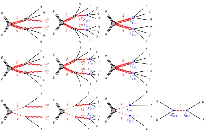
Figure 1: Production and decay processes for the three RPV SUSY models considered: (top) Gqq model, (middle) Gtt model, and (bottom) stop model. For each model the dominant process varies with increasing λ

coupling from left to right.

Three simplified models are considered:

Gqq model: the model contains light gluinos and the LSP, with non-zero λ

112

coupling and all other RPV couplings equal to zero. The gluinos are pair-produced and decay via off-shell squarks of the first and second generation. For low values of the RPV coupling the gluino decays as ˜ g → qq χ ˜

1

( q = u , d , s , c ) with the subsequent LSP decay, ˜ χ

1

→ qqq . For larger values of the coupling the

gluino can also decay as ˜ g → qqq . The masses of the first and second generation squarks are

assumed to be 3 TeV, while the masses of the other sparticles are set above 5 TeV, including third generation squarks.

Gtt model: the model contains light gluinos and the LSP, with non-zero λ

323

coupling and all other RPV couplings equal to zero. Values of the λ

323

coupling that are larger than the rest of the couplings are favored by the MFV hypothesis [22]. The gluinos are pair-produced and decay via off-shell top squarks. For low values of the RPV coupling the gluino decays as ˜ g → tt χ ˜

1

with the subsequent LSP decay, ˜ χ

1

→ tbs . For larger values of the coupling the gluino can also decay as ˜ g → tbs . The masses of the third-generation squarks are assumed to be 2.4 TeV; the masses of the other sparticles are set above 5 TeV, including first- and second-generation squarks. The choice for the masses of third-generation squarks is made to ensure that the prompt decay regime is reached before the branching fraction of ˜ g → tbs becomes non-negligible. A different choice is needed with respect to the Gqq model due to the presence of only two light right-handed squarks (stop and sbottom) and the phase-space suppression due to the top quark mass in the decay. Concurrence of direct RPV gluino decays and decays to a long-lived neutralino are possible for other choices of third-generation squark masses, but are not considered in this note.

Stop model: the model contains a light stop, ˜ t

, which is the right-handed superpartner of the top quark, and the LSP, with non-zero λ

323

coupling and all other RPV couplings equal to zero. Stops are pair-produced and decay as ˜ t

→ t χ ˜

1

for low coupling values, or ˜ t

→ bs for high coupling strengths. The LSP always decays as ˜ χ

1

→ tbs . The masses of the other sparticles are set above 3 TeV, but since the RPV decay proceeds via the right-handed stop, which is already part of the simplified model, there is no impact from this choice on the lifetime or branching ratios. For high coupling values single stop resonant production is also considered, pp → t ˜

→ bs , leading to a di-jet final state which may provide stronger constraints on the stop mass than pair production at the LHC [27]. Single stop resonant production followed by a decay to a top quark and neutralino, pp → t ˜

→ t χ ˜

1

→ ttbs , is not considered. The cross section for single production is more than two orders of magnitude higher than pair production for a stop mass of 500 GeV and for a fixed value of the coupling strength of λ

323

= 1, and evolves as ( λ

323

)

.

Figure 1 illustrates the production and decay modes considered in the three models, as a function of the λ

coupling strength. For very small values of the coupling the decay of the LSP can be displaced. For higher values of the coupling the decay of the LSP is prompt and the diagrams in the middle column occur with 100% branching ratio. For even higher values of the coupling the direct decay of the gluino or stop (right column) occurs with increasing branching ratio, reaching 100% for λ

values of order one. Direct decays of the gluino or stop are always prompt.

A theoretical upper limit on the coupling strength can be obtained by considering the renormalization group equations (RGE) of the superpotential parameters and by requiring the couplings to be perturbative up to the unification (GUT) scale, λ

( M

) < √

4 π . The limits obtained are λ

112

< 1 . 25 [28]

and λ

323

< 1 . 07 [29]. More stringent experimental limits on λ

112

can be obtained for particular choices of the sparticle masses. Low-energy measurements such as di-nucleon decay [30, 31] impose λ

112

. 5 · 10

q˜R) 1 TeV

g)˜ 1 TeV

. Combined with Eq. (2) lifetimes shorter than 100 ns are excluded for gluino masses up to 5 TeV, assuming a neutralino mass of 200 GeV. This lifetime limit scales as m( χ ˜

1

)

. No or only significantly weaker experimental limits can be set on λ

for other choices of i j k . The ATLAS analyses described in this note that provide limits on the Gqq model do not rely on b -quark identification, therefore the limits can be interpreted for any choice of λ

with i , 3. No experimental limit can be set on λ

323

.

Samples of Monte Carlo (MC) simulated events are used to model the signal. The response of the detector to signal events is modeled with the full ATLAS detector simulation [32] based on Geant4 [33]. All simulated events are overlaid with pile-up collisions simulated with the soft strong interaction processes of Pythia 8.186 [34] using the A2 set of tunable parameters (tune) [35] and the MSTW2008LO [36]

parton distribution function (PDF) set. Signal samples are generated at leading order with Mad- Graph5_aMC@NLO 2.3.3 [37] interfaced to Pythia 8.210, with up to two additional partons in the matrix element and using the A14 [38] tune for the underlying event. The parton luminosities are provided by the NNPDF23LO [39] PDF set.

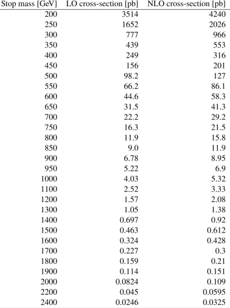
Signal pair-production cross-sections are calculated to next-to-leading order in the strong coupling con- stant, adding the resummation of soft-gluon emission at next-to-leading-logarithmic accuracy (NLO+NLL) [40–44]. The nominal cross-section and its uncertainty are taken from an envelope of cross-section pre- dictions using different PDF sets as well as different factorization and renormalization scales, as described in Ref. [45]. Although the models in this note specify the squark masses, contributions from squarks are not considered in the gluino pair-production cross-sections. The cross-section for single stop resonant production is computed at next-to-leading order in the strong coupling constant [27, 46].

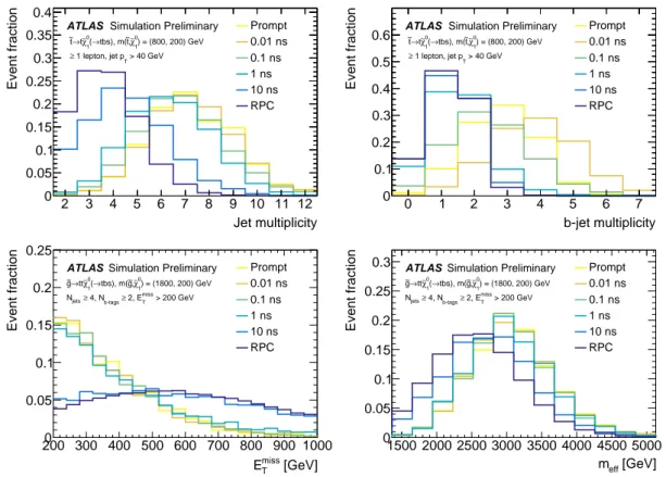
Figure 2 shows the impact of neutralino decays with different lifetimes on four representative distributions.

The number of jets increases once the neutralino decays are sufficiently prompt to be reconstructed in the calorimeter. A similar behavior is also seen in the number of b -tagged jets, but the maximum of the distribution occurs for a lifetime of 0.01 ns, where the additional decay length of the neutralino increases the b -tagging efficiency. Larger lifetimes reduce the number of b -tagged jets as the tracks are no longer reconstructed. The magnitude of the missing transverse momentum, E

T

, is reduced for shorter lifetimes as a larger fraction of decays happen within the detector volume; this reduction of the E

T

signal strongly reduces the sensitivity of RPC searches. The m

variable, defined as the scalar sum of lepton p

, jet p

and E

T

, increases slightly for events where the neutralino decays. This increase of the m

is caused by the momentum and mass of the neutralino being transmitted to the decay products: the scalar sum of the LSP decay products is always larger than the vectorial sum of the LSPs when they contribute to the E

T

.

2.2 R-hadron model

An additional simplified model inspired by Split SUSY is considered in this note, and referred to as the R -hadron model.

In this model, the gluino is kinematically accessible at LHC energies while the squarks have masses that are several orders of magnitude larger, in the PeV range. The gluino decays via a highly virtual intermediate state resulting in macroscopic lifetimes. Unlike the models described above, the long-lived particle is the gluino, which decays to a stable LSP via RPC couplings as shown in the first diagram of Figure 1. The LSP is assumed to be the lightest neutralino, ˜ χ

1

, with a mass of 100 GeV.

If the gluino lifetime is larger than the hadronization timescale of order 10

s, it will form a color-singlet

state with SM quarks and gluons. This bound state is referred to as an R -hadron. The mass of the

R -hadron is dictated by the mass of the gluino with additional contributions from the mass of the bound

SM particles and the binding energy associated with the hadron. The decays of the R -hadrons are largely

defined by the decay of the underlying gluino with a small amount of additional hadronic activity initiated

by the spectator partons.

Jet multiplicity

2 3 4 5 6 7 8 9 10 11 12

Event fraction

0 0.05 0.1 0.15 0.2 0.25 0.3 0.35 0.4

Prompt 0.01 ns 0.1 ns 1 ns 10 ns RPC ATLAS Simulation Preliminary

) = (800, 200) GeV 1

χ∼0 ,

~t tbs), m(

→ 1( χ∼0

→t

~t

> 40 GeV 1 lepton, jet pT

≥

b-jet multiplicity

0 1 2 3 4 5 6 7

Event fraction

0 0.1 0.2 0.3 0.4 0.5

0.6 ^Prompt

0.01 ns 0.1 ns 1 ns 10 ns RPC ATLAS Simulation Preliminary

) = (800, 200) GeV 1

χ∼0 ,

~t tbs), m(

→ 1( χ∼0

→t

~t

> 40 GeV 1 lepton, jet pT

≥

[GeV]

miss

ET

200 300 400 500 600 700 800 900 1000

Event fraction

0 0.05 0.1 0.15 0.2 0.25

Prompt 0.01 ns 0.1 ns 1 ns 10 ns RPC ATLAS Simulation Preliminary

) = (1800, 200) GeV 1

χ∼0 , g~ tbs), m(

→ 1( χ∼0

→tt g~

> 200 GeV miss 2, ET b-tags≥ 4, N jets≥ N

[GeV]

meff

1500 2000 2500 3000 3500 4000 4500 5000

Event fraction

0 0.05 0.1 0.15 0.2 0.25

0.3 _Prompt

0.01 ns 0.1 ns 1 ns 10 ns RPC ATLAS Simulation Preliminary

) = (1800, 200) GeV 1

χ∼0 , g~ tbs), m(

→ 1( χ∼0

→tt g~

> 200 GeV miss 2, ET b-tags≥ 4, N jets≥ N

Figure 2: Impact of neutralino decays with different lifetimes on the number of jets, number of b -tags, E

T

, and m

. All observables are shown at the reconstruction level with full simulation of the ATLAS detector.

Long-lived gluinos may hadronize into gluino-gluon balls ( ˜ gg ), gluino R -baryons ( ˜ gqqq ), or gluino R - mesons ( ˜ gq q ¯ ). In this note, a model of R -hadrons is employed as described in [47–49]. Signal samples are simulated with Pythia 6.428, with the AUET2B tune [35] parameters for the underlying event and the CTEQ6L1 [50] PDF set. Dedicated routines [49, 51, 52] for hadronization of heavy colored particles were used to simulate the production of R -hadrons, while the interactions of the R -hadrons with matter are handled by a dedicated simulation implemented in Geant4 [48].

The decay of the R -hadrons produces a final state with jets and E

T

. In the range of lifetimes where the decay of the R -hadron occurs within the inner detector, it can produce a displaced vertex signature for which dedicated searches exist [15]. For shorter lifetimes the number of sufficiently displaced vertices decreases and the signal resembles an RPC decay.

3 Analyses

A set of nine ATLAS searches that are sensitive to the models described in Section 2 are re-interpreted to set exclusion limits. None of the analyses saw significant excesses above the SM expectation in datasets ranging from 3.2 fb

to 37 fb

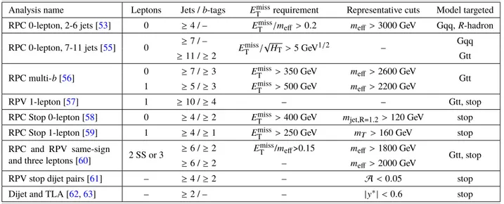
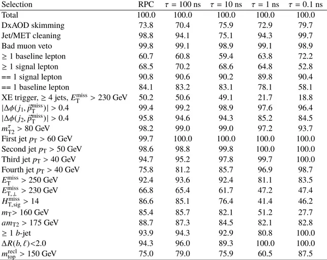
of 13 TeV proton–proton collision data. An outline of each of the included analyses is presented below, and the main characteristics of the most sensitive signal regions used can be found in Table 2. All the signal regions from the corresponding analyses are considered in the limit setting procedure, even if not listed in the table, except where explicitly noted. The requirements on E

T

or related variables are shown for each analysis, highlighting the different approach of RPC and RPV searches.

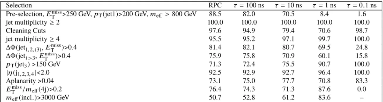
RPC 0-lepton, 2-6 jets: the analysis [53] searches for pair production of squarks or gluinos in final states with jets and E

T

, while vetoing electrons or muons. Two strategies are used: one based on the m

variable, and a second one based on recursive jigsaw reconstruction. Only m

SRs are considered here since they provide the best performance for the chosen neutralino mass. The search sets an exclusion limit on the gluino mass around 2 TeV in a simplified model with RPC, equivalent to the Gqq model considered in this note in the limit of a vanishingly small λ

coupling. The analysis rejects events from detector noise and non-collision background, if at least one of the two leading jets with p

> 100 GeV fails to satisfy the ‘Tight’ quality criteria, as described in Ref. [54]. This requirement places a cut on the jet charged particle fraction, defined as the ratio of the scalar sum of the p

of the tracks associated with the jet to the jet p

. This requirement introduces a high inefficiency for long-lived signals where displaced jets have no associated tracks, and is modified with respect to the original result. The modified requirement is based on the longitudinal calorimeter-sampling profile of these jets, and has been used in ATLAS searches for long-lived particles [15]. The two leading jets are required to have less than 96% of their energy in the electromagnetic calorimeter and less than 80% of their energy in a single calorimeter layer.

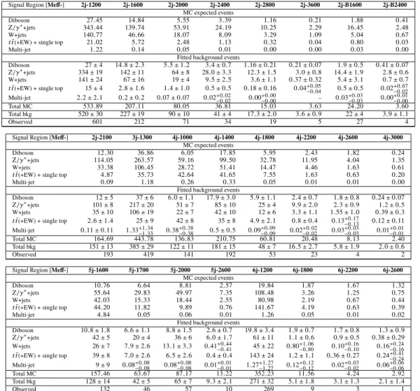
The signal and background yields in all signal and control regions show minimal changes, with all variations with respect to published results being below 4%, and below 2% for most regions. The full yields are provided in Appendix A. No excess of events is observed in any of the signal regions with the modified cleaning procedure.

RPC 0-lepton, 7-11 jets: the analysis [55] searches for gluinos which decay via long chains of particles, yielding a final state with high jet multiplicity and moderate E

T

. The analysis relies on a simplified E

T

significance, defined as E

T

/ √

H

, where H

is the scalar sum of all jet p

. The models targeted by this search do not map directly to the models considered in this note; in simplified models with long decay chains of SUSY particles, the analysis sets limits of up to 1.8 TeV on the gluino mass. Given the high jet multiplicity in events with moderate λ

coupling, and the possibility to obtain moderate E

T

due to misreconstruction of jets from late decays, this search has potential sensitivity to the Gqq and Gtt models.

RPC multi-b: the analysis [56] targets gluino production with the subsequent decay to top quarks and a neutralino, in a scenario equivalent to the Gtt model in the RPC limit. The search requires high jet and b -jet multiplicity, moderate E

T

and large m

. The final states with zero or one lepton are analyzed, and the sensitivity of the search is optimized using a two-dimensional shape-fit of the number of jets and m

. Gluino masses up to 2 TeV are excluded for a 200 GeV neutralino mass.

RPV 1-lepton: the analysis [57] searches for gluinos and stops in models with RPV couplings, yielding final states with at least one lepton, very high jet multiplicity and either no b -jets or many b -jets.

The search sets limit on the stop mass around 1 TeV in a model equivalent to the one considered in this note, in the regime where the LSP decay is prompt and assuming the stop decays only as t ˜ → t χ ˜

1

( → tbs). The search also sets limits on the gluino mass for two models that are similar to the Gtt model considered in this note, in the the regime where the LSP decay is prompt and the gluino decays only to ˜ g → tt χ ˜

1

, or only to ˜ g → tbs .

RPC stop 0-lepton, stop 1-lepton: both analyses [58, 59] search for stop pair production in a t¯ t + E

T

final state, with either both tops decaying hadronically, or one top decaying hadronically and the

other leptonically. Both analyses exploit jet reclustering to reconstruct boosted hadronic top decays,

while requiring that other quantities are incompatible with SM top quark pair production. Both searches set an exclusion limit on the stop mass around 1 TeV in a simplified model with RPC, equivalent to the stop model considered in this note in the limit of a vanishingly small λ

coupling.

RPC and RPV same-sign and 3-leptons (SS/3L): the analysis [60] covers a large variety of models including both RPC and RPV scenarios. Among the targeted scenarios are the three distinct regimes of the Gtt model described before, as well as final states compatible with the stop model with a prompt decay of the neutralino. The requirement of two same-sign or three leptons provides a powerful handle to suppress the Standard Model backgrounds, and allows the search to design SRs with and without an E

T

requirement, in order to cover RPC and RPV scenarios.

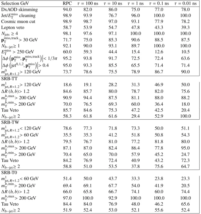
RPV stop dijet pairs: the analysis [61] targets stop pair production with the subsequent decay to a b - quark and s -quark, in a scenario equivalent to the stop model considered in this note in the regime with very high RPV coupling. The analysis requires two pairs of jets with large mass and low mass asymmetry, A . Stop masses up to 610 GeV are excluded assuming decays only to ˜ t → bs .

Dijet and TLA: For very high coupling values, single stop resonant production is also considered, pp → t ˜

→ bs , leading to a di-jet final state. The offline dijet search [62] and the trigger- level-analysis (TLA) dijet search [63] are reinterpreted to set limits in this regime. Both analyses search for a localized excess in the dijet mass spectrum, with small rapidity separation, | y

| .2 No signal samples are generated, and the limits on generic Gaussian resonances are reinterpreted. The procedure to reinterpret the Gaussian resonance limits is outlined in the Appendix of Ref. [64]. It requires the computation of acceptances suitable for the signal, which have been already computed in Ref. [27] and are applied here. The width-to-mass ratio is found to be 5 – 7% over the range of stop masses, and the experimental limits on a generic Gaussian resonance with width 7% are used for the reinterpretation.

4 Objects and systematic uncertainties

The analyses contained in this note are not designed to target long-lived signals, and as such use the standard ATLAS reconstruction of prompt objects. The object definition varies across analyses and can be found in the respective publications. Two choices that are common across analyses and have direct impact on displaced jets and leptons are discussed in the following.

To minimize the contribution from jets arising from pile-up interactions, the jets used by the analyses must satisfy a loose jet vertex tagger (JVT) requirement [65], where JVT is an algorithm that uses tracking and primary vertex information to determine if a given jet originates from the primary vertex. The chosen working point has an efficiency of 94% at a jet p

of 40 GeV and is nearly fully efficient at 60 GeV for jets originating from the hard parton–parton scattering. The JVT requirement is only applied to jets up to 60 GeV and within |η | < 2 . 4.3 Jets above this p

threshold will be accepted by the analyses even if they originate from displaced decays.

2

ATLAS uses a right-handed coordinate system with its origin at the nominal interaction point (IP) in the center of the detector and the z -axis along the beam pipe. The x -axis points from the IP to the center of the LHC ring, and the y -axis points upwards. Cylindrical coordinates (r, φ) are used in the transverse plane, φ being the azimuthal angle around the z -axis.

The pseudorapidity is defined in terms of the polar angle θ as η = − ln tan (θ/2 ) . Angular distance is measured in units of

∆R ≡

q (∆η)

+ (∆φ)

. The distance from the interaction point along the z -axis is denoted as |z| .

3

The RPV 1L analysis applies JVT to all jets within | η | < 2.4, regardless of their p

.

Analysis name Leptons Jets / b -tags E

T

requirement Representative cuts Model targeted RPC 0-lepton, 2-6 jets [53] 0 ≥ 4 / – E

T

/m

> 0 . 2 m

> 3000 GeV Gqq, R -hadron RPC 0-lepton, 7-11 jets [55] 0

≥ 7 / –

E

T

/ √

H

> 5 GeV

– Gqq

≥ 11 / ≥ 2 Gtt

RPC multi- b [56] 0 ≥ 7 / ≥ 3 E

T

> 350 GeV m

> 2600 GeV

Gtt

1 ≥ 5 / ≥ 3 E

T

> 500 GeV m

> 2200 GeV

RPV 1-lepton [57] 1 ≥ 10 / ≥ 4 – – Gtt, stop

RPC Stop 0-lepton [58] 0 ≥ 4 / ≥ 2 E

T

> 400 GeV m

> 120 GeV stop

RPC Stop 1-lepton [59] 1 ≥ 4 / ≥ 1 E

T

> 250 GeV m

> 160 GeV stop RPC and RPV same-sign

and three leptons [60] 2 SS or 3

≥ 6 / ≥ 2 E

T

/ m

>0.15 m

> 1800 GeV

Gtt, stop

≥ 6 / ≥ 2 – m

> 2000 GeV

RPV stop dijet pairs [61] – ≥ 4 / ≥ 2 – A < 0 . 05 stop

Dijet and TLA [62, 63] – ≥ 2 / – – |y

| < 0 . 6 stop

Table 2: Main characteristics of the most sensitive signal region per analysis. Only an illustrative subset of the cuts that define each signal region are included here. A dash (–) is used to indicate that the variable is not used in the analysis selection. The requirement of two same-sign leptons is denoted as SS. The variables used to illustrate the signal region selections are defined in the text.

The leptons used by the different analyses have requirements on their impact parameters in the final state.

The muon (electron) definition requires | z

sin θ | < 0 . 5 mm and | d

|/σ

< 3 ( 5 ) , therefore no displaced leptons are picked up by the analyses.

The performance of the reconstruction and calibration algorithms on displaced signals is studied, and dedicated uncertainties are developed to cover possible discrepancies in the MC simulation of such topologies. All analyses implement the full set of uncertainties described in the respective publication. In addition, the analyses that are sensitive to signals with sizable lifetime include two dedicated uncertainties to account for possible modeling differences between data and simulation of displaced signals, described in this Section. These uncertainties are only applied to signal samples, as the background events in all signal regions originate from promptly-decaying processes.

4.1 Jet energy scale uncertainties for displaced jets

Given the difficulty to study the response of displaced jets in data, an MC-based prescription is designed to evaluate additional uncertainties for displaced jets. The jet response, defined as the p

ratio of the reconstructed jet over the truth jet, is studied in order to understand the effects of jet displacement on the jet energy scale (JES) and the jet energy resolution (JER).

The procedure of construction and investigation of the jet response follows the strategy described in [66].

The jet response is computed from reconstructed jets geometrically matched to truth jets using the distance

measurement ∆R . Truth jets are labeled as originating from a long-lived particle by performing a p

-

dependent ∆R matching to the decaying neutralino or R -hadron. Only isolated jets are used to compute

the jet response to avoid disturbing effects from near-by jets. Reconstructed jets are required to have no

additional reconstructed jets within a cone of ∆R = 0 . 6. Only one truth jet is allowed to be present within

a cone of ∆R = 1 . 0 of the reconstructed jet. Since reconstructed jets are always assumed to originate from

the primary vertex, a geometric correction to θ and φ is applied to the direction of the reconstructed jets, according to the position of the displaced vertex from the long-lived particle. This correction is performed only to improve the matching to truth jets, and the jet response is computed with respect to the uncorrected jet.

The deviation from unity of the observed jet response is affected by the volume of the calorimeter (1 . 0 < R < 3 . 9 m and 2 . 8 < | z| < 6 m) and is taken as an extra systematic uncertainty, and parameterized as a function of the radial decay length of the long-lived particle. The assigned uncertainty is below the percent level for radial decay lengths below 1 m, grows linearly reaching 30% at 1.6 m, and remains approximately constant until it reaches the outside surface. The jet reconstruction efficiency decreases quickly while approaching the outside surface, dropping below 10% for radial decay lengths larger than 3 m.

Usually only a difference between data and MC in the response is considered as an uncertainty [66].

The use of the full response difference is however a conservative choice, since several studies of jets and calorimeter clusters in data with properties similar to displaced jets have shown much smaller levels of disagreement than the uncertainties assigned in this analysis. For example, the longitudinal shower profile in current GEANT physics lists agrees well between data and MC [67]; the modeling of the energy in clusters located in the hadronic calorimeter agrees well with the data [66]; and studies of jets with a large fraction of their energy deposited only in the hadronic calorimeter show that their p

is well modelled [68].

While the applied uncertainty is thus conservative with respect to these studies in data, it does not strongly affect the sensitivity of the searches.

Similarly to what is the done for JES, an extra systematic for JER was considered by studying the evolution of the width of the jet response as a function of the radial decay length. However, the variation of the JER is smaller than the uncertainty associated to it, and is not considered as an additional systematic.

4.2 b-tagging uncertainties for displaced jets

The b -tagging efficiency is expected to be affected by the additional decay length induced by the long-lived particle. For decay lengths of the order of millimeters the b -tagging efficiency improves, while it degrades rapidly once the jets originate after the innermost layer of silicon pixels (IBL), 31 mm < R

< 40 mm [69]. The average b -tagging efficiency for jets originating from the decay of an LSP with τ

= 0 . 01 ns is about 85% for b -jets and 20% for light-jets, compared to 77% and < 1% respectively in simulated t t ¯ events. The contribution from mis-tagged light-jets is therefore not negligible. In order to evaluate the systematic uncertainties associated to the b -tagging of displaced jets a bottom-up approach is used, where the underlying tracking observables are adjusted in MC samples to match those found in data, and the effect is then propagated to the b -tagging observables.

Measurements of tracking performance in both data and simulation are performed. The modeling of the

tracking, such as impact-parameter resolution, track reconstruction efficiency and fake-rate, is adjusted in

simulation to match the data. The b -tagging algorithm is re-evaluated on the adjusted MC to compute

the modified b -tagging efficiency, and the uncertainties on the tracking modeling are propagated to the

efficiency. The difference between nominal and adjusted efficiency is not used to correct the nominal

simulation but is instead taken as an additional uncertainty.

The extra systematic uncertainty assigned is 10% (20%) for event selections with ≥ 2 b -tags ( ≥ 4 b - tags) and signal lifetimes of 1 ns. The size of the uncertainty decreases (increases) for shorter (longer) lifetimes.

4.3 Missing transverse momentum uncertainties

The missing transverse momentum is reconstructed from the negative vector sum of the transverse momenta of the hard objects in the event, and a soft term built from high-quality tracks that are associated with the primary vertex but not with the physics objects. Variations on the hard objects due to systematic uncertainties are propagated to the missing transverse momentum, including the additional JES uncertainty for displaced jets discussed before. Uncertainties on the soft term are taken into account but do not require additional terms due to displaced signals since it is built only from tracks associated with the primary vertex.

The performance of the missing energy trigger and its dependence with the LSP lifetime is evaluated in simulation and no impact on the trigger efficiency turn-on is observed. The online and offline E

T

definitions do not introduce significant differences in the treatment of displaced jets, therefore no additional trigger systematic is considered.

5 Results

Results are provided in the context of three RPV SUSY benchmark models and the R -hadron model discussed in Section 2, using the nine ATLAS analyses described in Section 3. In all cases except for the dijet analyses, the profile likelihood-ratio test [70] is used to establish 95% confidence intervals using the CL

prescription [71]. In the dijet analyses a Bayesian procedure is used to set 95% credibility-level upper limits on generic Gaussian resonances [62]. Individual limits from each analysis are reported, and no combination is performed due to substantial overlaps in signal region definitions and in order to highlight the performance of the approach of each analysis.

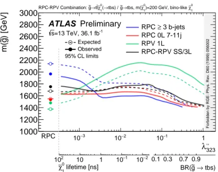
Figure 3 shows the observed and expected lower gluino mass limits obtained in the Gqq model, as a function of the neutralino lifetime and the gluino branching ratio, as well as the equivalent λ

112

coupling strength. The RPC 0L 2-6 jet analysis sets the strongest limits on this model in the RPC and low λ

112

regime. The sensitivity of the analysis falls off rapidly as the lifetime of the ˜ χ

1

decreases and the decays to jets reduce the E

T

. The RPC 0L 7-11 jet analysis, also sets limits, but the moderate jet multiplicity of the signal reduces its efficiency in the small RPV coupling region, while the lack of E

T

reduces its efficiency in the large RPV coupling region. Gluino masses up to 2 TeV are excluded for a neutralino lifetime of 100 ns, and up to 1 TeV for a lifetime of 1 ns. While the generated model had non-zero values only for λ

112

, the limits apply for any λ

with i , 3. No limits are set for λ

112

' 10

. Previous searches in all-hadronic final states have set a limit of about 1.2 TeV on the gluino mass when considering the prompt decay ˜ g → qq χ ˜

1

[72], and 0.9 TeV when considering the prompt and direct decay to light quarks, g ˜ → qqq [73].

Figure 4 shows the observed and expected lower gluino mass limits obtained in the Gtt model, as a function of the neutralino lifetime and the gluino branching ratio, as well as the equivalent λ

323

coupling strength.

The RPC multi- b analysis sets the strongest limits in the RPC limit and for low values of λ

323

. As the

coupling increases and the ˜ χ

1

lifetime decreases, the E

T

in the final state reduces substantially and weakens the limits. Unlike in the Gqq model, though, the high top quark multiplicity in the final state still leads to some E

T

through leptonic decays, which allows the analysis to continue to be sensitive to even higher values of λ

323

. The limits degrade further as the ˜ g decay transitions from the ˜ χ

1

cascade to a direct RPV decay, reducing the jet and top quark multiplicities compared to the direct RPV case and thereby lowering the sensitivity. The RPV 1L analysis sets the strongest limits for moderate and high values of λ

323

. The analysis was optimized for the high-multiplicity final state resulting from the ˜ g → tt χ ˜

1

, χ ˜

1

→ tbs cascade, and indeed its sensitivity is strongest when the branching ratio to this final state is maximized. The peak sensitivity is achieved for signals with τ

≈ 10

ns, due to the improvement in b -tagging efficiency. For higher values of λ

323

, the final state jet multiplicity is reduced, weakening the limits; for lower values of λ

323

, the displaced signature results in some particles escaping the detector and again reducing the final state jet multiplicity. The entire λ

323

range is covered effectively by the various analyses; the weakest limits occur for λ

323

≈ 2 · 10

, where the appreciable ˜ χ

1

lifetime leads to displaced signatures which none of the existing analyses exploit, and at λ

323

≈ 1, where the ˜ g decays directly to fewer jets and is more difficult to separate from the background. The strongest limits occur in the RPC limit for the RPC multi- b analysis, and at λ

323

≈ 3 · 10

for the RPV 1L analysis.

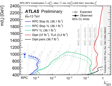
Figure 5 shows the observed and expected lower stop mass limits obtained in the stop model as a function of λ

323

. Contours of ˜ χ

1

lifetime and branching ratios of direct decays, ˜ t → bs , are overlaid since they depend on both the coupling value and the stop mass. In the RPC regime, and for low values of λ

323

, the RPC stop 0L and stop 1L analyses set the strongest limits. The reliance on high E

T

signatures quickly reduces the sensitivity at even moderate values of λ

323

and ˜ χ

1

lifetime. The RPV 1L analysis, in green, begins setting limits for slightly higher values of λ

323

, setting its strongest limits near λ

323

≈ 10

. The gap between the stop 0L/1L and RPV 1L analyses can potentially be closed by new searches utilizing displaced vertices or displaced leptons. At very high values of λ

323

, the stop dijet pairs analysis, in black, sets limits for low values of the stop mass. The single stop resonant production, accessible via the dijet analyses, sets extremely strong limits for these high values of λ

323

. The weakest limits in the plane occur in the transitions between analyses; the strongest are set by the dijet analysis, which excludes stops of mass 2.4 TeV at λ

323

≈ 1.

Figure 6 shows the observed and expected lower gluino mass limits obtained in the R -hadron model, as a function of the lifetime of the R -hadron.4 The re-interpretation of the 0L 2-6 jet analysis places the strongest limits for the lowest lifetime values, and provides strong limits until the decay of the R -hadron reaches the calorimeters. Results from previous ATLAS publications [15, 16, 18, 74] are also shown, excluding gluino masses up to 1.6 TeV over the full range of R -hadron lifetimes. While the sensitivity of analyses searching for the direct interaction of the R -hadron with the detector can be affected by the choice of R -hadron spectrum, the result presented here from the 0L 2-6 jet analysis is insensitive to these effects.

4

Contrary to Figures 3–5, the lifetime increases from left to right on Figure 6.

112

λ

1000 1200 1400 1600 1800 2000 2200 2400 2600 2800 3000

) [GeV] g~ m(

RPC 0L 2-6 jets RPC 0L 7-11 jets

ATLAS Preliminary

1

χ∼0

)=200 GeV, bino-like

1

χ∼0

qqq, m(

→ g~ qqq) /

→

1( χ∼0

→qq g~ RPC-RPV Combination:

=13 TeV, 36.1 fb-1

s

−3 2 10 10−

−1

10 1

2 10 10

lifetime [ns]

1

χ∼0

RPC

Forbidden by RGE: Phys. Lett. B 346 (1995) 69

−4

10 10⁻³ 10⁻²

Expected Observed 95% CL limits

Figure 3: Exclusion limits for the Gqq model as a function of λ

112

and m( g) ˜ . Expected limits are shown with dashed lines, and observed as solid. The RPC-limit is shown on the leftmost part of the axes.

323

λ

1000 1200 1400 1600 1800 2000 2200 2400 2600 2800 3000

) [GeV] g~ m(

3 b-jets

≥ RPC RPC 0L 7-11j RPV 1L

RPC-RPV SS/3L

ATLAS Preliminary

1

χ∼0

)=200 GeV, bino-like

1

χ∼0

tbs, m(

→ g~ tbs) /

→

1( χ∼0

t

→t g~ RPC-RPV Combination:

=13 TeV, 36.1 fb-1

s

−2 1 10 10−

1

2 10 10

lifetime [ns]

1

χ∼0

RPC

Forbidden by RGE: Phys. Rev. D60 (1999) 056002

−3

10 10⁻² 10⁻¹ 1

0.1 0.3 0.7 0.9 tbs)

→ g~ BR(

Expected Observed 95% CL limits

Figure 4: Exclusion limits for the Gtt model as a function of λ

323

and m( g) ˜ . Expected limits are shown with dashed lines, and observed as solid. The RPC-limit is shown on the leftmost part of the axes, while the region λ

323

> 1 . 07

is forbidden by constraints from the renormalization group equations.

323

λ

400 600 800 1000 1200 1400 1600 1800 2000 2200 2400 ) [GeV]

t ~ m(

ns

2

= 10 τ

-2 ns = 10 τ

-3 ns = 10 τ ns

0

= 10 τ ns

1

= 10 τ

-1 ns = 10 τ

bs)=95%→1t~ BR(

bs)=25%→1t~BR( bs)=75%→1t~ BR(

bs)=50%→1t~ BR(

bs)=5%→1t~ BR(

RPC

Forbidden by RGE: Phys. Rev. D60 (1999) 056002

-1) RPC Stop 0L (36.1 fb

-1) RPC Stop 1L (36.1 fb

-1) RPV 1L (36.1 fb

-1) ), TLA (3.2 fb Dijet (37 fb-1

-1) Dijet pairs (36.7 fb

ATLAS Preliminary

−4

10 10⁻³ 10⁻² 10⁻¹ 1

1

χ∼0

)=200 GeV, bino-like

1

χ∼0

bs, m(

→

~t tbs) /

→

1( χ∼0

→t

~t RPC-RPV Combination:

=13 TeV s

Expected Observed 95% CL limits

Figure 5: Exclusion limits for the stop model as a function of λ

323

and m(˜ t ) . Expected limits are shown with dashed lines, and observed as solid. The RPC-limit is shown on the leftmost part of the axes, while the region λ

323

> 1 . 07 is forbidden by constraints from the renormalization group equations. No expected limit is shown for the dijet and TLA results.

[ns]

2

τ

10

10

1 10 10

10

10

) [GeV] g~ m(

500 1000 1500 2000 2500 3000

Expected Observed

-1)

=13 TeV, 36 fb s

RPC 0L 2-6 jets (

-1)

=13 TeV, 33 fb s

Displaced vertices (

-1)

=13 TeV, 3.2 fb s

Pixel dE/dx (

-1)

=13 TeV, 3.2 fb s

Stable charged (

-1)

=7,8 TeV, 5.0,23 fb s

Stopped gluino ( 95% CL limits

Preliminary ATLAS

) = 100 GeV

1

χ∼0

; m(

1

χ∼0

→ qq (R-hadron) g~

γ=1) β η=0,

(r for Beampipe Inner Detector Calo MS

Prompt Stable

τ [m]

c

−3

10 10

10

1 10 10

10

10

Figure 6: Exclusion limits for the R -hadron model, as a function of the R -hadron lifetime and the gluino mass. The

area below the curves is excluded. Results from previous ATLAS publications covering the full range of R -hadron

lifetimes are shown. The dots represent results for which the particle is assumed to be prompt or stable. In this

context, stable means escaping the detector.

6 Conclusions

This note describes the reinterpretation of existing ATLAS analyses in models with variable R -parity

coupling strength and R -hadron lifetime. Four simplified models, three targeting RPV scenarios and one

targeting R -hadrons, are analyzed. The large variations in final state, and therefore in sensitivity, as a

function of the R -parity coupling strength motivate a thorough examination of the full ATLAS SUSY

program’s coverage. Different degrees of sensitivity are observed as a function of λ

: in the gluino

model with large branching fractions to top quarks, gluinos are excluded up to masses of 1.8 TeV, over

the full range of lifetime and RPV coupling strengths. In the gluino model with decays to first and second

generation quarks, the differences are even more striking: for low values of the coupling, gluino masses

are excluded up to 2.0 TeV, but at high values of λ

no limits are set. The stop model shows large

variations in the limits as well: stop masses up to 2.4 TeV can be excluded at high values of λ

, but no

limits can be established for values of λ

≈ 10

, equivalent to neutralino lifetimes around 1 ns. Gluinos

in models with short lived R -hadrons can also be excluded up to masses of 2.0 TeV by the re-interpretation

of existing RPC-targeting analyses.

References

[1] H. Miyazawa, Baryon Number Changing Currents, Prog. Theor. Phys. 36 (1966) 1266.

[2] R. Ramond, Dual Theory for Free Fermions, Phys. Rev. D 3 (1971) 2415.

[3] Yu. A. Golfand and E. P. Likhtman,

Extension of the Algebra of Poincare Group Generators and Violation of p Invariance, JETP Lett. 13 (1971) 323, Pisma Zh. Eksp. Teor. Fiz. 13 (1971) 452.

[4] A. Neveu and J. Schwarz, Factorizable dual model of pions, Nucl. Phys. B 31 (1971) 86.

[5] A. Neveu and J. Schwarz, Quark Model of Dual Pions, Phys. Rev. D 4 (1971) 1109.

[6] J. Gervais and B. Sakita, Field theory interpretation of supergauges in dual models, Nucl. Phys. B 34 (1971) 632.

[7] D. V. Volkov and V. P. Akulov, Is the Neutrino a Goldstone Particle? Phys. Lett. B 46 (1973) 109.

[8] J. Wess and B. Zumino, A Lagrangian Model Invariant Under Supergauge Transformations, Phys. Lett. B 49 (1974) 52.

[9] J. Wess and B. Zumino, Supergauge Transformations in Four-Dimensions, Nucl. Phys. B 70 (1974) 39.

[10] P. Fayet, Supersymmetry and Weak, Electromagnetic and Strong Interactions, Phys. Lett. B 64 (1976) 159.

[11] H. K. Dreiner, An Introduction to explicit R-parity violation,

Adv. Ser. Direct. High Energy Phys. 21 (2010) 565, arXiv: hep-ph/9707435 [hep-ph] . [12] R. Barbier et al., R-parity violating supersymmetry, Phys. Rept. 420 (2005) 1,

arXiv: hep-ph/0406039 [hep-ph] .

[13] G. F. Giudice and A. Romanino, Split supersymmetry, Nucl. Phys. B 699 (2004) 65, arXiv: hep-ph/0406088 , Erratum: Nucl. Phys. B 706 (2005) 65.

[14] N. Arkani-Hamed and S. Dimopoulos, Supersymmetric unification without low energy supersymmetry and signatures for fine-tuning at the LHC, JHEP 06 (2005) 073, arXiv: hep-th/0405159 .

[15] ATLAS Collaboration, Search for long-lived, massive particles in events with displaced vertices and missing transverse momentum in

√ s = 13 TeV pp collisions with the ATLAS detector, (2017), arXiv: 1710.04901 [hep-ex] .

[16] ATLAS Collaboration, Search for metastable heavy charged particles with large ionization energy loss in pp collisions at

√ s = 13 TeV using the ATLAS experiment, Phys. Rev. D 93 (2016) 112015, arXiv: 1604.04520 [hep-ex] .

[17] ATLAS Collaboration, Search for direct top squark pair production in events with a Higgs or Z boson, and missing transverse momentum in

√ s = 13 TeV pp collisions with the ATLAS detector, JHEP 08 (2017) 006, arXiv: 1706.03986 [hep-ex] .

[18] ATLAS Collaboration, Search for long-lived stopped R-hadrons decaying out of time with pp collisions using the ATLAS detector, Phys. Rev. D 88 (2013) 112003,

arXiv: 1310.6584 [hep-ex] .

[19] J. Alwall, M.-P. Le, M. Lisanti, and J. G. Wacker,

Searching for Directly Decaying Gluinos at the Tevatron, Phys. Lett. B 666 (2008) 34, arXiv: 0803.0019 [hep-ph] .

[20] J. Alwall, P. Schuster, and N. Toro,

Simplified Models for a First Characterization of New Physics at the LHC, Phys. Rev. D 79 (2009) 075020, arXiv: 0810.3921 [hep-ph] .

[21] D. Alves et al., Simplified Models for LHC New Physics Searches, J. Phys. G 39 (2012) 105005, arXiv: 1105.2838 [hep-ph] .

[22] C. Csaki, Y. Grossman, and B. Heidenreich, MFV SUSY: A Natural Theory for R-Parity Violation, Phys. Rev. D 85 (2012) 095009, arXiv: 1111.1239 [hep-ph] .

[23] H. K. Dreiner and G. G. Ross, R-parity violation at hadron colliders, Nucl. Phys. B 365 (1991) 597.

[24] W. Porod, SPheno, a program for calculating supersymmetric spectra, SUSY particle decays and SUSY particle production at e+ e- colliders, Comput. Phys. Commun. 153 (2003) 275,

arXiv: hep-ph/0301101 [hep-ph] . [25] W. Porod and F. Staub,

SPheno 3.1: Extensions including flavour, CP-phases and models beyond the MSSM, Comput. Phys. Commun. 183 (2012) 2458, arXiv: 1104.1573 [hep-ph] .

[26] F. Staub, SARAH 4 : A tool for (not only SUSY) model builders,

Comput. Phys. Commun. 185 (2014) 1773, arXiv: 1309.7223 [hep-ph] .

[27] A. Monteux, New signatures and limits on R-parity violation from resonant squark production, JHEP 03 (2016) 216, arXiv: 1601.03737 [hep-ph] .

[28] J. L. Goity and M. Sher, Bounds on ∆B = 1 couplings in the supersymmetric standard model, Phys. Lett. B 346 (1995) 69, arXiv: hep-ph/9412208 [hep-ph] .

[29] B. C. Allanach, A. Dedes, and H. K. Dreiner, Two loop supersymmetric renormalization group equations including R-parity violation and aspects of unification, Phys. Rev. D 60 (1999) 056002, arXiv: hep-ph/9902251 [hep-ph] , Erratum: Phys. Rev. D 86 (2012) 039906.

[30] N. Zwane, Long-Lived Particle Searches in R-Parity Violating MSSM, J. Phys. G 44 (2017) 105003, arXiv: 1505.03479 [hep-ph] .

[31] M. Litos et al., Search for Dinucleon Decay into Kaons in Super-Kamiokande, Phys. Rev. Lett. 112 (2014) 131803.

[32] ATLAS Collaboration, The ATLAS Simulation Infrastructure, Eur. Phys. J. C 70 (2010) 823, arXiv: 1005.4568 [physics.ins-det] .

[33] S. Agostinelli et al., GEANT4: A Simulation toolkit, Nucl. Instrum. Meth. A 506 (2003) 250.

[34] T. Sjöstrand, S. Mrenna, and P. Z. Skands, A Brief Introduction to PYTHIA 8.1, Comput. Phys. Commun. 178 (2008) 852, arXiv: 0710.3820 [hep-ph] . [35] ATLAS Collaboration, Further ATLAS tunes of Pythia 6 and Pythia 8,

ATL-PHYS-PUB-2011-014, 2011, url: http://cds.cern.ch/record/1400677 . [36] A. Sherstnev and R. Thorne, Parton Distributions for LO Generators,

Eur. Phys. J. C 55 (2008) 553, arXiv: 0711.2473 [hep-ph] .

[37] J. Alwall et al., The automated computation of tree-level and next-to-leading order differential cross sections, and their matching to parton shower simulations, JHEP 07 (2014) 079,

arXiv: 1405.0301 [hep-ph] .

[38] ATLAS Collaboration, ATLAS Pythia 8 tunes to 7 TeV data, ATL-PHYS-PUB-2014-021, 2014, url: https://cds.cern.ch/record/1966419 .

[39] R. D. Ball et al., Parton distributions with LHC data, Nucl. Phys. B 867 (2013) 244, arXiv: 1207.1303 [hep-ph] .

[40] W. Beenakker, R. Hopker, M. Spira, and P. Zerwas,

Squark and gluino production at hadron colliders, Nucl. Phys. B 492 (1997) 51, arXiv: hep-ph/9610490 .

[41] A. Kulesza and L. Motyka,

Threshold resummation for squark-antisquark and gluino-pair production at the LHC, Phys. Rev. Lett. 102 (2009) 111802, arXiv: 0807.2405 .

[42] A. Kulesza and L. Motyka, Soft gluon resummation for the production of gluino-gluino and squark-antisquark pairs at the LHC, Phys. Rev. D 80 (2009) 095004, arXiv: 0905.4749 . [43] W. Beenakker et al., Soft-gluon resummation for squark and gluino hadroproduction,

JHEP 12 (2009) 041, arXiv: 0909.4418 .

[44] W. Beenakker et al., Squark and gluino hadroproduction, Int. J. Mod. Phys. A 26 (2011) 2637, arXiv: 1105.1110 .

[45] C. Borschensky et al.,

Squark and gluino production cross sections in pp collisions at

√ s = 13, 14, 33 and 100 TeV, Eur. Phys. J. C 74 (2014) 3174, arXiv: 1407.5066 .

[46] T. Plehn, Single stop production at hadron colliders, Phys. Lett. B 488 (2000) 359, arXiv: hep-ph/0006182 [hep-ph] .

[47] R. Mackeprang and A. Rizzi, Interactions of Coloured Heavy Stable Particles in Matter, Eur. Phys. J. C 50 (2007) 353, arXiv: hep-ph/0612161 .

[48] R. Mackeprang and D. Milstead,

An Updated Description of Heavy-Hadron Interactions in GEANT-4, Eur. Phys. J. C 66 (2010) 493, arXiv: 0908.1868 [hep-ph] .

[49] A. C. Kraan, Interactions of heavy stable hadronizing particles, Eur. Phys. J. C 37 (2004) 91, arXiv: hep-ex/0404001 .

[50] J. Pumplin et al.,

New generation of parton distributions with uncertainties from global QCD analysis, JHEP 07 (2002) 012, arXiv: hep-ph/0201195 [hep-ph] .

[51] G. R. Farrar and P. Fayet, Phenomenology of the Production, Decay, and Detection of New Hadronic States Associated with Supersymmetry, Phys. Lett. B 76 (1978) 575.

[52] M. Fairbairn et al., Stable massive particles at colliders, Phys. Rept. 438 (2007) 1, arXiv: hep-ph/0611040 [hep-ph] .

[53] ATLAS Collaboration, Search for squarks and gluinos in final states with jets and missing transverse momentum using 36 fb

of

√ s =13 TeV pp collision data with the ATLAS detector,

(2017), arXiv: 1712.02332 [hep-ex] .