5 Conservation Equations for Turbulent Flows

5 Conservation Equations for Turbulent Flows

5.1 Conservation Equations for Mean Variables in a Turbulent Flow

The most fundamental approach to describe – and hence simulate – a hydro- dynamic flow consists of setting up a set of conservation equations for mass, energy and momentum and trying to find a solution to this set of non-linear coupled differential equations. It is well known that for atmospheric flows this set of equations has, generally, no analytical solution. Therefore, either they are simplified (e.g., by neglecting ‘unimportant’ terms) until a solution is possible or they are solved numerically on a grid. In the latter approach the differentials are replaced by differences and for example a term like

€

∂χ ∂x will become

€

(χ

− χ

) Δ x , where

€

χ is just some general variable and

€

Δ x represents the grid spacing between grid point i and grid point i+1

. This general approach is employed in essentially all atmospheric models ranging from global climate and weather prediction models down to very detailed local flow models. In principle, this is also the case for models aiming at describing a turbulent flow. However, as we have seen, turbulence continuously covers all scales from a few millimeters up to the dimensions of the entire boundary layer (Table 2.1) and this would make it necessary to employ extremely high spatial and hence temporal resolution when attempting to fully resolve turbulence in such a model

. Therefore, for any practical application the concept of Reynolds decomposition and averaging is applied to the conservation equations, which separates the turbulence scales from those of the mean flow (Chapter 3.3). Models, which use this type of Reynolds averaged conservation equations are referred to as Ensemble models, thus emphasizing the fact that Reynolds averaging is employed as a surrogate for a (desired) ensemble mean (see Chapter 3).

The set of conservation equations as they are well known are summarized in Table 5.1. Before starting to look at the individual members of this set in some detail, we set out the general procedure how to proceed with Reynolds decomposition and averaging:

Step 1: Formulate the conservation equation (Table 5.1).

Step 2: Simplify where appropriate.

Step 3: Apply Reynolds decomposition.

1 There are many different ways to achieve this ‘discretisation’ on a grid such as finite differences (a variety of which is the simple example presented above), finite volumes or finite elements and even more numerical techniques to optimally set up such a scheme.

However it is not the focus of the present book to go into detail in this respect.

2 Indeed this is done in research applications over very limited domains (mostly for technical flows, like modelling the flow through a valve) and called direct numerical simulation (DNS).

If the turbulence is partly resolved by filtering the conservation equations at an appropriate wave-number in phase space, this is referred to as Large Eddy Simulation (LES). The latter approach constitutes the most advanced modelling technique available for present-day computing power.

- 2 -

Step 4: Reynolds-average the resulting equation to obtain the conservation equation for the mean flow variable.

Step 5: Express the result of step 4 in flux form (if appropriate).

Step 6: Subtract the result of step 4 from that of step 3 to obtain the conservation equation for the fluctuating variable.

Step 7: Multiply the result of step 6 with another fluctuating variable to obtain an equation for the corresponding second order moment.

Step 8: Reynolds-average the result of step 7 to obtain the conservation equation for this mean second order moment.

(Step 9: Repeat steps 6-8 to obtain conservation equations for even higher order moments).

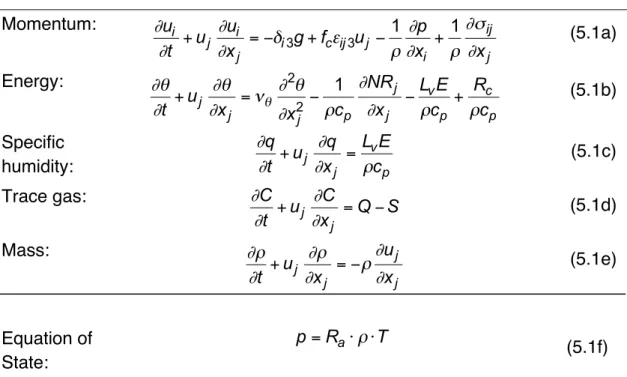
Table 5.1: Conservation equations for atmospheric flows Momentum:

€

∂ u

∂ t + u

∂ u

∂ x

= − δ

^g + f

ε

^u

− 1 ρ

∂ p

∂ x

+ 1 ρ

∂σ

∂ x

(5.1a) Energy:

€

∂θ

∂t + u

∂θ

∂x

= ν

∂

θ

∂x

− 1 ρc

∂NR

∂x

− L

E ρc

+ R

ρc

^(5.1b)

Specific

humidity:

€

∂ ^q

∂ t + u

∂ ^q

∂ x

= L

E

ρ c

(5.1c)

Trace gas:

€

∂ ^C

∂ t + u

∂ ^C

∂ x

= Q − S (5.1d)

Mass:

€

∂ρ

∂ ^{t + u}

∂ρ

∂ ^x

^{= −} ρ ∂ u

∂ ^x

(5.1e)

Equation of State:

€

p = R

⋅ ρ ⋅ T

(5.1f)

g: acceleration due to gravity;

€

f_c Coriolis parameter; p pressure,

€

σ shear stress tensor;

€

ε_ijk=1 if (i,j,k) cyclic, =1 if (i,j,k) anti-cyclic and zero otherwise;

€

ν_θ thermal viscosity;

€

NR_j component of net radiation in j-direction;

€

L_v latent heat of evaporation,

€

R_c energy released from chemical reactions (or other processes); E evaporation; Q source for trace gas; S sink for trace gas;

€

R_a

‘ideal gas’ constant for air (

€

≡R/M_a≈286Jkg⁻¹K⁻¹, where

€

M_a is the molecular weight of dry air).

5.1.1 Equation of State for ideal gases

Starting from eq. (5.1f), applying Reynolds decomposition yields

€

p + p' = R

( ρ T + ρ T '+ ρ ' T + ρ ' T') . (5.2)

Reynolds averaging according to the rules outlined in Table 3.2 then leads to

€

p = R

( ρ ^T + ρ ^{' T'). (5.3)}

The fluctuations of density and temperature are highly correlated, but still since

€

T ' = O( 1K) and

€

ρ '= O(

€

10

kgm

) the covariance term in (5.2) becomes much smaller than the first term on the rhs so that

€

p ≈ R

( ρ T ) (5.4)

to good accuracy. Subtracting (5.4) from (5.2) yields an equation for the fluctuating pressure

€

p' = R

( ρ T '+ ρ ' T + ρ ' T') . (5.5)

Equation (5.5) can easily be divided by

€

p / R

= ρ T and brought to the form

€

p' p = T '

T + ρ' ρ + ρ' T'

ρ T ^{. (5.6)}

Both the fluctuating density and temperature are much smaller than their mean counterparts, so that the last term on the rhs of (5.6) can safely be neglected. We know that

€

p' = O( 0.1hPa) and hence

€

p' /p = O(

€

10

) while

€

T ' /T = O(

€

10

) (see above: temperature fluctuations). Therefore, from (5.6) it follows that also the density fluctuations must be the same order of magnitude as the temperature fluctuations and hence

€

ρ ' ρ = − T '

T ^{. (5.7)}

This relation is, first of all, obvious since warm eddies will have a smaller density. Second it will help us to replace the density fluctuations as they appear in some of the equations below to be replaced by the more easily obtainable temperature fluctuations.

5.1.2 Continuity Equation (Conservation of Mass)

The incompressibility assumption states that the density changes are much smaller than the divergence of the flow field under typical atmospheric conditions and can thus be neglected. Indeed this is a very good approximation for essentially all ABL flows. Therefore, steps 3,4 and 6 to eq.

(5.1e) yields

€

∂ u

∂ x

= 0 ; ∂ u'

∂ x

= 0 (5.8)

Equation (5.8) states that the continuity equation is (to good accuracy) valid for both the mean flow and the velocity fluctuations.

We employ the continuity equation to derive the so-called flux form of the advection terms (see step 5 above). The advection term for a general variable

€

χ ^is

€

u

∂χ ∂ ^x

and we therefore have with the aid of (5.8)

∂ ^(u

χ ⁾

∂ ^x

⁼ χ ∂ ^u

∂ ^x

^{+ u}

∂χ

∂ ^x

^{= u}

∂χ

∂ ^x

(5.9)

- 4 -

The rhs of (5.9) is what we usually will encounter in the various conservation equations while the lhs is what we want, i.e. the flux divergence for any quantity

€

χ . According to (5.8) we can use (5.9) for both the mean and fluctuating terms.

5.1.3 Conservation of momentum

The three equations (summation on index i) for conservation of momentum on a rotating Earth are generally referred to as Navier-Stokes Equations and are repeated here for convenience:

€

∂u

∂ t + u

∂u

∂ x

= −δ

g + f

ε

u

− 1 ρ

∂p

∂ x

+ 1 ρ

∂σ

∂ x

I II III IV V VI ^(5.1a) The terms denote, respectively: the local temporal change (I); the advection term (II); acceleration due to gravity (III); the Coriolis term (IV); the pressure gradient (V) and the shear stress due to molecular friction (VI).

Step 2: Simplifications and Assumptions

The most straightforward assumption is that of a Newtonian fluid (see BOX

‘Tools to describe atmospheric flows’ in Chapter 2). With this, term (IV) becomes

€

1 ρ

∂σ

∂x

= ν ∂

u

∂ x

^{. (5.10)}

Note that in this formulation we have already used the assumption of incompressibility.

The next simplification that is usually invoked in describing the conservation of momentum deals with density fluctuations and is known as Boussinesq Approximation. To better understand what it is all about we consider the conservation equation for the vertical velocity component (i=3) for a horizontally homogeneous flow, in which the viscosity is constant:

€

dw

dt = −g − 1 ρ

∂ ^p

∂ ^{z +} ν ∂

^w

∂ ^z

(5.11) (Note that we have employed the total temporal derivative – simply for convenience). We now apply Reynolds decomposition and multiply the whole equation with

€

ρ = ρ '+ ρ

€

( ρ '+ ρ ) d(w + w')

dt = −( ρ '+ ρ )g − ∂ ^(p + p')

∂ ^{z +} η ∂

^(w + w')

∂ ^z

, (5.12)

where

€

η = ρν (eq. (2.6)). Dividing (5.12) by the mean density yields

€

(1+ ρ'

ρ ) d(w + w') dt = − ρ'

ρ g - g − 1 ρ

∂p

∂ z − 1 ρ

∂p'

∂ z + ν ∂

(w + w')

∂ z

< - - - - -- >

, (5.13)

where we have employed that

€

η /( ρ '+ ρ ) ≈ η / ρ = ν . The gravity and the pressure gradient terms (underlined with double arrow in eq. (5.13) are by far the largest (on the order of

€

10ms

). These two terms can, in fact, be rearranged to yield the hydrostatic equation (

€

∂ p = − g ρ∂ z). Often for large- scale flows it can be assumed that it is in hydrostatic equilibrium. This is justified if no steep topography or other obstacles are producing local pressure effects and usually this assumption may hold down to a spatial grid- resolution of around 10km. Under the hydrostatic assumption these two terms cancel each other in (5.13)

. Analyzing the orders of magnitude of the remaining terms in (5.13) shows that

€

1+ ρ' ρ ≈ 1 and hence the density fluctuations can be neglected as compared to the mean. However,

€

ρ' ρ also appears in connection with

€

g and this term proves to be the second largest term after the two leading terms, which cannot be neglected. The Boussinesq approximation therefore demands

Neglect the density fluctuations with respect to the mean (

€

ρ ' ρ ≈ 0 ), but not in the gravity term.

A practical way to introduce the Boussinesq approximation in a set of equations (e.g. for a numerical model) therefore consists of replacing the density by the mean density (

€

ρ → ρ ) and the acceleration due to gravity

€

g by

€

g(1 − θ ' θ ) (where we have used (5.7))

.

The Boussinesq approximation is valid if the so-called shallow convection conditions are fulfilled (Stull 1988), i.e. if

- the domain height (in our case: the boundary layer height) is much smaller than the scale height (

€

≈ 8km ), i.e. that height where the pressure in an isothermal atmosphere has dropped to its e

fraction.

- the density fluctuations (and hence the temperature fluctuations and the pressure fluctuations – see discussion in connection with eq. (5.6)) can be neglected with respect to their mean

- the flow is incompressible

- the stratification is unstable (or slightly stable at most).

Applying all these assumptions to (5.1a) yields

€

∂ u

∂t + u

∂ u

∂x

= −δ

(g − θ '

θ ) + f

ε

u

− 1 ρ

∂ p

∂x

+ ν ∂

u

∂x

^{. (5.14)}

3 Note that what is usually referred to as a hydrostatic model, essentially makes this scale analysis of (5.13) and only keeps the hydrostatic equation. Thus the conservation equation for vertical velocity component is simply this hydrostatic equation.

4 This is basically what we have done in eqs. (5.11) to (5.13).

- 6 -

Steps 3/4: Reynolds decomposition and averaging

Reynolds decompositions has, of course, not to be applied to the gravity term (this has been done already in the Boussinesq approximation) and we obtain after applying the Reynolds averaging rules

€

∂ u

∂ t + u

∂ u

∂ x

+ u'

∂ u'

∂ x

= −δ

g + f

ε

u

− 1 ρ

∂ p

∂ x

+ ν ∂

u

∂ x

^{. (5.15)} We note, first of all, that the Boussinesq approximation has no effect at all on the conservation equation for mean momentum. It will only become instrumental in the conservation equations for higher order moments.

Comparing further (5.15) with (5.1a) reveals that – apart from replacing all variables by their mean – only one additional term (three terms per equation by invoking the Einstein summation, of course) has appeared in (5.15), i.e. the third on the lhs.

Step 5: Flux form

Using (5.9) on this new term in (5.15) yields

€

∂ u

∂t + u

∂ u

∂x

+ ∂

∂x

(u

u

) = −δ

g + f

ε

u

− 1 ρ

∂ p

∂x

+ ν ∂

u

∂x

^{. (5.16)} The new terms in (5.16) are related to the divergence of the turbulent fluxes (covariances). Even if there is only one additional term between (5.1a) and (5.16) due to the introduction of turbulence through Reynolds decomposition and averaging, it is clear that in the ABL, where the turbulent fluxes are substantial this is a crucial step for an appropriate description of the flow.

5.1.4 Conservation of Energy

We start with the first law of thermodynamics to show that conserving (internal) energy essentially (in the atmospheric boundary layer) means conserving potential temperature. The first law of thermodynamics reads

€

δQ = c

dT − pdα . (5.17)

where

€

δ ^Q is the increment of energy,

€

c

the specific heat at constant volume and

€

α = 1/ ρ . With the aid of the equation of state and writing out the total differential

€

d α , (5.17) can be written as

€

δ Q = c

dT − R

T dp

p . (5.18)

Now, considering the total differential of the potential temperature we find – by introducing the definition of potential temperature –

€

d θ = ( p

p )

dT − κ ^{T ( p}

p )

p

p

dp = θ ^{( dT}

T − R

c

dp p )

. (5.19)

Therefore, the product

€

dθ Tc

θ = c

dT − R

T dp

p (5.20)

is equal to the rhs of (5.18). Using again the definition of the potential temperature we have

€

δ Q = T

θ c

d θ = ( p

p )

c

d θ

. (5.21)

For

€

p

= 1000hPa and

€

p = 900hPa, say,

€

δ ^Q ≈ 0.97c

d θ ^{, and for}

€

p = 800hPa the factor is about 0.94. Thus to good accuracy the conservation equation for potential temperature can be taken as a surrogate for conserving (inner) energy.

In the conservation equation for potential temperature (5.1b)

€

∂θ

∂t + u

∂θ

∂x

= ν

∂

θ

∂x

− 1 ρc

∂NR

∂x

− L

E ρc

+ R

ρc

^(5.1b)

the terms on the rhs are due to, respectively: the molecular diffusion of heat;

the divergence of radiation (

€

NR

= the component of net radiation in j- direction); phase changes of water; any other source/sink such as from chemical reactions (

€

R

denoting just a generic energy portion released or required for such a process). The last three are all ‘essentially external’, i.e.

independent of the flow itself. They may therefore be summarized to one

€

1 ρ c

∂ ^NR

∂ x

− L

E ρ c

+ R

ρ c

≡ 1

ρ c

QR (5.22)

Finally, applying Reynolds decomposition and averaging as well as bringing the result into flux form yields

€

∂θ

∂ t + u

∂θ

∂ x

+ ∂

∂ x

(u'

θ ') = ν

∂

θ

∂ x

+ 1

ρ c

QR (5.23)

Again, as for the conservation equation for momentum, the only difference between the original equation (5.1b) and the final result (5.23) is, that the variables now are mean variables and the additional term on the lhs, which describes the divergence of the turbulent flux of sensible heat.

5.1.5 Mass Conservation for a trace constituent The conservation of specific humidity (

€

q) and an arbitrary trace gas such as a

pollutant are treated in the same way because at this stage we do not have

any simplifications to introduce. Therefore steps 3,4 and 5 are applied all

together and the conservation equations for a mean trace constituent in a

turbulent flow read

- 8 -

€

∂ ^q

∂ t + u

∂ ^q

∂ x

+ ∂

∂ x

(u

q') = L

E

ρ c

(5.24)

€

∂ ^C

∂ t + u

∂ ^C

∂ x

+ ∂

∂ x

(u

C') = Q − S

. (5.25)

5.1.6 Summary of first order conservation equations

Table 5.2 summarizes all the conservation equations we have to deal with in order to describe a mean turbulent flow. All the equations differ from the original ones (Table 5.1) only through the fact that the variables are mean variables now and, most important, the additional flux divergence terms.

Having noticed the importance of turbulent fluxes in general within the ABL, we observe then that the ‘turbulence enters the conservation equations for mean variables’ through the Reynolds decomposition procedure and manifests itself as the often even dominating flux divergence term in each of the equations.

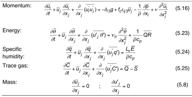
Table 5.2: Conservation equations for mean variables in turbulent flows.

Assumptions are the Boussinesq approximation, incompressible flow and a Newtonian fluid.

Momentum:

€

∂ u

∂ ^{t + u}

∂ u

∂ ^x

⁺

∂

∂ ^x

^(u

'

u

) = − δ

g + f

ε

u

− 1 ρ

∂ p

∂ ^x

⁺ ν ∂

u

∂ x

(5.16)

Energy:

€

∂θ

∂ t + u

∂θ

∂ x

+ ∂

∂ x

(u'

θ') = ν

∂

θ

∂ x

+ 1

ρ c

QR ^(5.23) Specific

humidity:

€

∂ ^q

∂ ^{t + u}

∂ ^q

∂ ^x

⁺

∂

∂ ^x

^(u

'

q') = L

E

ρ ^c

^(5.24)

Trace gas:

€

∂ ^C

∂ ^{t + u}

∂ ^C

∂ ^x

⁺

∂

∂ ^x

^(u

'

C') = Q − S (5.25) Mass:

€

∂ u

∂ ^x

^{= 0 ;}

∂ u'

∂ ^x

^{= 0}

(5.8)

Equation of State:

€

p = R

ρ T

(5.4)

In Chapter 2 it was stated that the turbulent diffusion is some

€

10

larger than the molecular diffusion (Table 2.2). Hence the terms describing the molecular diffusion can safely be neglected as compared to the turbulent flux divergence (they are only kept here for completeness).

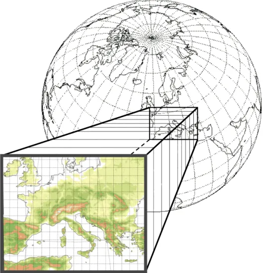
The equations summarized in Table 5.2 constitute the basis for setting up a

model for boundary layer flows. These equations are solved on a grid (i.e. at

each grid point) as shown in Fig. 5.1 by replacing the derivatives with finite differences. Restricting ourselves for the moment to the pure flow (without trace gas, but with specific humidity taken into account) we have seven equations and seven mean variables (i.e., first order moments). This system could numerically be solved. However, in addition there are a number of second order moments (covariances) introduced through the Reynolds decomposition. These additional variables may be treated by introducing conservation equations for higher-order moments (see Section 5.1.7).

Alternatively, we may use similarity theory (Chapter 4) to directly describe these ‘new’ variables. Since most of the similarity relations are in one way or the other dependent on surface fluxes (Chapter 4), many models employ surface layer similarity theory (MOST) to estimate the surface fluxes from the information at the first model level. In other words it is assumed that the first model level is within the SL.

Figure 5.1 Conceptual sketch showing a model grid domain as embedded

(nested) in a larger (global) domain to provide the boundary and initial

conditions.

- 10 -

For the Situation given in Fig. 5.2 one may assume that – for a given integration time – all the conservation equations have been solved and a set of mean variables is available at the first model level. In very general terms for the variable

€

χ we may express its surface flux

€

w' χ'

= −C

u r

L1

(χ

− χ

) . (5.26)

Here,

€

C

is the exchange coefficient and the subscript ‘L1’ denotes the first model level. If

€

χ is the horizontal velocity component, the exchange coefficient is called drag coefficient and usually gets the subscript ‘D’:

€

w' u'

= − C

u

. (5.27)

Using MOST

€

C

can easily be determined to

€

C

= k

ln z

z

− Ψ

(z / L)



  

 

(5.28)

To evaluate the Obukhov length (eq. 4.12) a first guess can be based on the surface fluxes

from the previous time step and an iterative procedure is used to solve for

€

L . Since this is usually considered to be too cpu-time demanding,

€

Ψ

is then approximated in a simplified form (e.g., Louis, 1979).

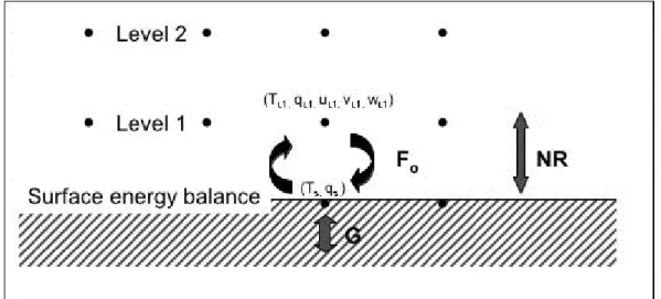
Figure 5.2 First model levels in a numerical model. The surface fluxes

€

F

(e.g., for momentum, latent and sensible heat) are determined using the prognostic variables at the first model level,

€

χ

, and those at the surface,

€

χ

. The velocity components vanish at the surface by definition. The surface temperature and humidity are usually determined using the surface energy balance and hence the radiation balance (net radiation, NR) and the ground heat flux, G.

5 The turbulent surface heat flux is determined in an analogous manner with

€

χ=θ in (5.26).

5.1.7 Conservation equations for higher order moments

Having introduced a number of ‘new variables’ in the conservation equations for the mean flow variables through Reynolds decomposition one may want to find conservation equations for those. This is done, in general, by steps 6 to 8 in the general outline at the beginning of Section 5.1. Here, it is demonstrated on the example of the momentum equation.

The starting point in this exercise is eq. (5.16)

€

∂u

∂t + u

∂u

∂x

+ ∂

∂x

(u

u

) = −δ

g + f

ε

u

− 1 ρ

∂p

∂x

+ ν ∂

u

∂x

^{. (5.16)} This has – according to step 6 – to be subtracted from the fully expanded momentum equation, which is written out here for convenience

€

∂ ^u

∂ ^{t +}

∂ ^u

∂ ^{t + u}

∂ ^u

∂ ^x

^{+ u}

∂ ^u

∂ ^x

^{+ u}

^'

∂ ^u

∂ ^x

^{+ u}

^'

∂ ^u

∂ ^x

⁼

− δ

^g + δ

θ ' θ



  

  g + f

ε

^u

+ f

ε

^u

− 1 ρ

∂ p

∂ x

− 1 ρ

∂ p'

∂ x

+ ν ∂

u

∂ x

+ ν ∂

u

∂ x

(5.29) Subtracting (5.16) from (5.29) yields a prognostic equation for the fluctuating wind components

€

∂ ^u

∂ ^{t + u}

∂ ^u

∂ ^x

^{+ u}

^'

∂ ^u

∂ ^x

^{+ u}

'

∂ ^u

∂ ^x

⁼ + δ

θ '

θ



  

  g + f

ε

u

− 1 ρ

∂ p'

∂ x

+ ν ∂

u

∂ x

(5.30)

We now multiply (5.30) by

€

2u

to yield

€

2u

∂ u

∂ t + 2u

u

∂ u

∂ x

+ 2u

u

' ∂ u

∂ x

+ 2u

u

∂ u

∂ x

= +2 δ

u

θ '

θ



  

  g + 2f

ε

u

u

− 2 u

ρ

∂ p'

∂ x

+ 2 ν u

∂

u

∂ x

(5.31)

Note that with this multiplication we have introduced a summation. While in (5.30) the subscript ‘i’ was not summed (i.e., referring to three equations according to Einstein summation rules), eq. (5.31) now contains this subscript in each term twice so that summation has to be invoked. We further note that, e.g.,

€

∂ ^u'

∂ ^t = 2u

⋅ ∂ ^u

∂ ^t and eq. (5.31) can be rearranged

- 12 -

€

∂ u'

∂ t + u

∂ u'

∂ x

+ 2u'

u'

∂ u

∂ x

+ u

∂ u'

∂ x

= +2 δ

u

θ ^'

θ



  

  g + 2f

ε

u

u

− 2 u

ρ

∂ ^p'

∂ ^x

^{+ 2} ν u

∂

^u

∂ ^x

^(5.32)

This is still summed. Reynolds averaging then leads to

€

∂ ^u'

∂ ^{t + u}

∂ ^u'

∂ ^x

^{+ 2u}

'

u

∂ ^u

∂ ^x

^{+ u}

'

∂ ^u'

∂ ^x

⁼

+ 2 δ

^u

θ ' θ



  

  g + 2f

ε

^u

^u

− 2 u

ρ

∂ p'

∂ ^x

^{+ 2} ν ^u

∂

u

∂ x

(5.33)

Finally, bringing (5.33) into flux form and rearranging yields

€

∂ u'

∂t + u

∂ u'

∂x

= − 2u

u

∂ u

∂x

− ∂ u

u'

∂x

+ 2 δ

u

θ ' θ



  

  g + 2f

ε

u

u

− 2

ρ u'

∂ p'

∂x

+ 2 ν u'

∂

u'

∂x

^(5.34)

Due to the summation introduced in step 6, equation (5.34) is, first of all, the conservation equation for TKE (cf. the definition of TKE, eq. 3.25). We will come back to its meaning and application in Chapter 6. We only note here, that the Boussinesq approximation has now its effect in that the buoyancy term remains even if otherwise density fluctuations are neglected.

If the Einstein summation convention is interpreted only weakly, (5.34) may also yield 3 conservation equations for the three velocity variances. What does this mean? Grouping all the terms in (5.34) with

€

i = 1 ,

€

i = 2 and

€

i = 3 together, denoting these groups with A, B and C, respectively and finally bringing all the terms to one side of the equation, (5.33) can be expressed as

€

A + B + C = 0 . This is consistent with

€

A = 0 (

€

i = 1 ),

€

B = 0 (

€

i = 2 ) and

€

C = 0 (

€

i = 3 ), although this is only one special solution to the full equation. Still, this weak interpretation of the summation rules is used to obtain the conservation equations for the velocity variances:

€

∂ ^u'

∂ ^{t + u}

∂ ^u'

∂ ^x

^{= − 2u}

'

u

∂ ^u

∂ ^x

⁻

∂ ^u

^u'

∂ ^x

+ 2f

u

u

− 2 ρ

∂ u'

p'

∂ x

+ 2 ρ ^p'

∂ u'

∂ x

− 2 ν ^u _'1 ∂

u'

∂ x

(5.35)

€

∂ u'

∂ ^{t + u}

∂ u'

∂ ^x

^{= −2u}

'

u

∂ u

∂ ^x

⁻

∂ u

u'

∂ ^x

−2f

u

u

− 2 ρ

∂ ^u'

^p'

∂ ^x

⁺ 2 ρ ^p'

∂ ^u'

∂ ^x

^{− 2} ν u'

∂

^u'

∂ ^x

^(5.36)

€

∂ ^u'

∂ ^{t + u}

∂ ^u'

∂ ^x

^{= −2u}

'

u

∂ ^u

∂ ^x

⁻

∂ u

u'

∂ ^x

+ 2g θ ^u

'

θ

− 2 u

u

∂ ^u

∂ ^x

⁻ 2 ρ

∂ u'

p'

∂ ^x

⁺ 2 ρ ^p'

∂ u'

∂ ^x

^{− 2} ν ^u'

∂

u'

∂ ^x

^(5.37)

5.2 Closure Problem and Closures

In the previous sections of this chapter the conservation equations for the first moments (mean variables) in a turbulent flow were derived with the result that through Reynolds decomposition second order variables entered the problem.

As a possible solution it was offered to use conservation equations for those second order moments as additional constraints to solve the set of equations.

However, inspecting eq. (5.33) as one example for the second order moment equations, it becomes immediately clear that even more unknowns (third order moments) appear in these equations. In fact, it can be shown that the higher the order of moments for which conservation equations are derived, the larger the number of unknowns becomes. This dilemma – the higher the order of moments for which conservation equations are taken into account, the more unknowns – is called the closure problem. The set of equations is never closed.

So, very generally when trying to describe a turbulent flow through its conservation equations we always get into trouble: either we have to resolve the entire spectrum of turbulent fluctuations and this leads to enormous requirements of computing resources (cpu-problem). Alternatively, we treat the turbulence in a statistical manner and introduce Reynolds decomposition and averaging – and this leads to the closure problem. The former problem may be solvable in some distant time when computers will have become even much more powerful than they are today. The latter, the closure problem, is solved by making a closure assumption. A closure is characterized by its order:

Closure of order

€

n : conservation equations are taken into account for statistical moments up to order

€

n . The moments of order

€

n + 1 , which appear in these equations are found from parameterizations.

For example, a closure of first order would use the equations of Table 5.2 for

the mean variables (first order moments) and parameterize all the (co-)

variances (second order moments). If we denote the j

moments of order n

- 14 - with

€

M

and allow for

€

P

n+1

parameters, the unknown moments of order

€

n + 1 can be parameterized through

Closure of order

€

n :

€

M

= f (M

, M

, ...M

, P

n+1

) . Clearly, not all the moments of order

€

n must be used in every parameterization for the higher order moments – but they may.

Parameterizations may be looked at as a ‘short cut’ for complicated physics or, sometimes, as an emergency solution for unknown physics. In finding these parameterizations, however, one has to follow some basic rules:

- The parameterization must be consistent with the unknown in terms of physical units and tensor symmetries.

- The parameterization must be invariant with respect to transformations (e.g. coordinates)

- Global constraints and conservation principles for the unknown must not be violated.

According to the above notation, the conservation equations of Table 5.2 are sufficient for a first-order closure. If, for example, a model is to be set up for the flow in the SL, Monin-Obukhov similarity theory (Chapter 4) may be used to derive the parameterizations

for the second order moments.

So, which closure should be chosen? One may think that ‘the higher order the closure, the better’. This is certainly not true. We know quite little for moments higher than third (sometimes fourth) order. So, any parameterization becomes pure guesswork. So the highest realistic and feasible order for turbulence closures is two (sometimes three). In the following we will introduce some of the most common and most frequently used closure schemes.

5.2.1 First order closure

In first order closures all the second order moments must parameterized. We first note that this means that in such a framework the entire information on turbulence for this flow is then buried in the closure. Still, due to its relative simplicity this closure is the most often used and hence best investigated closure approach. Due to the commonly used notation (see below) first order closure is often referred to as ‘K-Theory’. We introduce this approach by looking at the exchange of momentum.

In analogy to molecular diffusion where the local shear stress is described as proportional to the deformation rate (see box ‘Tools to describe atmospheric flows’ in Chapter 2)

€

σ

= ρνs

=: ρν ∂u (

∂x

+ ∂u

∂ xi ) ^(5.38)

6 This is why MOST is sometimes referred to as ‘zero order closure’ (no conservation equations at all) – to be consistent with the closure notation. However, it is clear that the similarity principles are more than just parameterizations.

a similar approach if followed for the Reynolds stress tensor

€

τ because its (off diagonal) elements describe the turbulent transport of momentum due to the turbulent shear stress:

€

τ

ρ ^{= − (K}

⁾

( ∂ u

∂ x

+ ∂ u

∂ _xi ) ^{, (5.39)}

where the minus sign is introduced for convenience to take into account the fact that the turbulent flux is usually directed opposite to the mean gradients.

The subscript ‘m’ stands here for momentum and the exchange coefficient

€

(K

)

is most generally also a two dimensional tensor. Its elements are sometimes also referred to as ‘turbulent diffusivity’ or ‘eddy viscosity’. For an ideal horizontally homogeneous flow with its x-axis aligned to the mean wind direction (5.38) simplifies to

€

τ

ρ ^{= u'}

^u'

^{= −(K}

⁾

∂ u

∂ x

(5.40)

and

€

(K

)

is often denoted simply as

€

K

.

It is first noted that ‘K-Theory’ is a local approach in that the turbulent fluxes at a certain height are parameterized by the gradient of the mean variables at the same level. It is hence valid if small-scale turbulence prevails, i.e. if the eddies are not much larger than the height range where this gradient occurs.

In the ABL this is the case in the SL at least if the stratification is not too convective, in the entire neutral ABL and to some extent also in the SBL.

Equation (5.39) can be generalized to other turbulent fluxes that need to be parameterized according to

€

w'a' = −K

∂ a

∂ x

^{, (5.41)}

where ‘

€

a ’ may denote the potential temperature (

€

θ ), the specific humidity (

€

q ) or the concentration of a trace constituent of the atmosphere (

€

C ). In the form of (5.40) and (5.41) and with

€

i = 3 first order closure or ‘K-Theory’ is most commonly employed.

Clearly, with the ‘K-approach’ we have only shifted the problem of parameterizing the unknown turbulent fluxes towards specifying the unknown

€

K . The simplest approach would certainly be to assume

€

K = const. but this proves not to be the best assumption (e.g., Stull 1988). In the early 20

century Prandtl proposed the so-called mixing length approach for momentum

€

K

= l

∂ ^u

∂ ^x

^{, (5.42)}

and v. Kàrmàn has introduced a simple parameterization for the mixing

length, l = kz (with k ≈ 0.4 the v. Kàrmàn constant). If we insert this in (5.40),

use the definition of the friction velocity (3.42) and rearrange we obtain

- 16 -

€

∂ u

∂ x

z u

= 1

k ^{. (5.43)}

Thus the Prandtl / v. Kàrmàn approach is consistent with Monin-Obukhov Similarity Theory (MOST) for neutral stratification (cf. equation (4.14)) or, in other words, the latter is an extension of the former for general stability. Note, however, that in the framework of MOST for neutral stratification,

€

K

= kzu

and thus the exchange coefficient is itself dependent on the surface flux of momentum.

For each regime the similarity relations (Chapter 4) may therefore help to find appropriate formulations for the exchange coefficients. Stull (1988) gives an overview (his Table 6-4). We may add here a word of caution. Even if parameterizations for the exchange coefficients can be found for convective conditions (as for example in Stull’s table), first order closure is not appropriate in the ML. We will come back to this issue below (Section 5.2.3).

5.2.2 Closure of order 1.5

In the literature one not only finds closures with an integral number order but also mixed (fractional) orders. As an example the so-called

€

e − ε ^closure model is briefly outlined, which is of order 1.5. In this approach the turbulent fluxes are parameterized according to (5.41) but the model for the exchange coefficients uses the turbulent kinetic energy (

€

e ) and the dissipation rate for TKE (

€

ε )

€

K

∝ e

ε ^{, (5.44)}

and solves prognostic equations for these variables (e.g., equation (5.34) for TKE – see also Chapter 6). This approach (apart from being dimensionally consistent) thus recognizes the fact the TKE and the dissipation rate of TKE are both important variables for the turbulent exchange. This closure is therefore first order in principle, but some higher order moments are also taken into account (hence the notation). Note that there are a number of similar 1.5 order turbulence closure models in the literature, which employ a similar approach as described here, but with various extensions or additional constraints being invoked.

5.2.3 Non-local closure

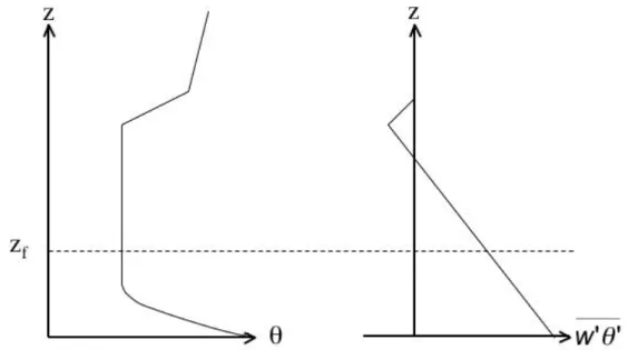
Up to now all the closures presented were local in the sense that a turbulent flux (or any other higher order moment) at a certain height is parameterized using the gradient of the mean variable at this very height. In Fig. 5.3 typical profiles of the potential temperature and the turbulent flux of sensible heat are sketched to show the failure of such an approach in the CBL. At any height

€

z

outside the surface layer it is readily seen that

€

∂θ ∂ z ≈ 0 while the turbulent flux of sensible heat is different from zero. Thus any formulation for the exchange coefficient of the type (5.42) must fail. This is due to the fact that in the CBL large eddies of order

€

z

dominate the turbulent exchange and the

local gradient of the mean potential temperature is not a good measure to represent this process.

A pragmatic way to solve this problem is to introducing a ‘counter gradient term’ in the parameterization for, e.g., the turbulent heat flux, viz.

€

w' θ ^' = − K

( ∂θ

∂ ^{z −} γ

^{) , (5.45)}

which may itself be parameterized from using some knowledge of the CBL (e.g., Holtslag and Boville 1993). Such approaches may be used if computing efficiency is important as for example in global atmospheric models.

Figure 5.3 Sketch of potential temperature and turbulent heat flux profiles in the CBL.

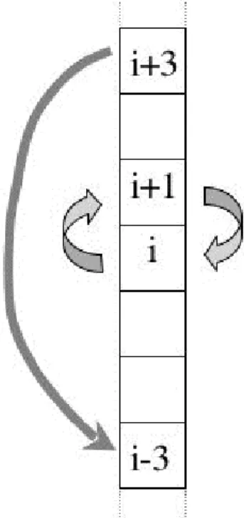
Another non-local closure model is known as Transilient Turbulence Theory and is described in detail by Stull (1988). Its basic idea consists of requiring that the turbulent exchange at any point in space may be, in principle, influenced from any other point in the domain. If the domain is sub-divided into boxes (Fig. 5.4) small eddies would be represented by exchange between neighboring boxes while large eddies are described by exchange between distant boxes. Similar to a ‘K-Theory’ approach the exchange is then described as proportional to the difference in the mean property between all the possible pairs of boxes. For this the mixing of a property

€

C in a column with

€

n boxes is formally described as how this property at position i changes (after a time step

€

Δ t , say) due to exchange with all the other boxes:

C

(t + Δ t ) = M

(t, Δ t ) ⋅

j=1 n

∑ C

(t ). (5.46)