Simulation of Recent Southern Hemisphere Climate Change
Nathan P. Gillett
1* and David W. J. Thompson
2Recent observations indicate that climate change over the high latitudes of the Southern Hemisphere is dominated by a strengthening of the circumpolar westerly flow that extends from the surface to the stratosphere. Here we demonstrate that the seasonality, structure, and amplitude of the observed climate trends are simulated in a state-of-the-art atmospheric model run with high vertical resolution that is forced solely by prescribed stratospheric ozone depletion. The results provide evidence that anthropogenic emissions of ozone- depleting gases have had a distinct impact on climate not only at stratospheric levels but at Earth’s surface as well.
Recent climate change in the Southern Hemi- sphere (SH) is marked by a strengthening of the circumpolar westerlies in both the strato- sphere (1– 4) and the troposphere (1, 4). In the stratosphere, the trends are largest during the spring months (2–5); in the troposphere, they are largest during the summer months (4). In both the stratosphere and the tropo- sphere, the trends are reflected as a bias in the leading mode of SH extratropical variability, the so-called Southern Hemisphere annular mode (SAM) (6).
Recently, Thompson and Solomon (4) (hereafter TS) have argued that the trend in the tropospheric component of the SAM during the summer months is consistent with forcing by stratospheric ozone depletion. Their argument is based on the observations that (i) the strato- spheric polar vortex has strengthened during the spring season over the past few decades in response to the development of the Antarctic ozone hole (2,3) and (ii) anomalies in the SH stratospheric vortex during the spring season tend to descend in time and are reflected as similarly signed anomalies in the tropospheric circulation during the early summer months (4, 7,8). TS went on to argue that the summertime trends in the SAM are consistent with the ob- served cooling of Antarctica during the summer season and, to a lesser extent, the warming observed over the Antarctic Peninsula [see (9) for a recent synopsis of observed trends in Antarctic surface temperature].
Here we use results from a state-of-the-art atmospheric model with high vertical resolution coupled to a mixed-layer ocean model to test the hypothesis outlined in TS. We demonstrate that the seasonality, vertical structure, horizon- tal structure, and amplitude of the simulated
response to prescribed SH stratospheric ozone depletion bear a striking resemblance to the observed trends not only in the SH stratosphere but in the SH troposphere as well. The study follows from results reported in previous stud- ies (10 –12), which also examine the response of the SAM to prescribed stratospheric ozone losses. However, none of these studies examine the seasonally varying vertical structure of the response, assess the attendant impacts on sur- face temperature, or provide a quantitative comparison with observations. Additionally, two of the studies (10,11) draw from experi- ments run with prescribed sea-surface temper- atures (which provide an additional constraint on the tropospheric response), and the experi- ments in (12) are based on exaggerated levels of stratospheric ozone depletion (13).
We used simulations from a 64-level ver- sion of the third Hadley Centre slab model, denoted HadSM3-L64. Details of the model are given in (12). The model has a horizontal resolution of 2.5°latitude by 3.75°longitude, a 50-m-deep mixed-layer ocean, a dynamic and thermodynamic sea-ice model, and a 64-level atmosphere extending up to 0.01 hPa (14).
The impact of ozone depletion on the SH circulation was assessed by comparing two simulations run with different seasonally varying ozone distributions; all other external variables were held fixed. The control simu-
lation was run with a seasonally varying re- construction of preindustrial ozone based on an observed climatology (15); the perturbed simulation was integrated with prescribed stratospheric ozone losses based on observed trends over the 18-year period 1979 to 1997 (16) (Fig. 1). The response of the model to the prescribed stratospheric ozone depletion is examined by differencing temperatures, geopotential heights, and wind velocities be- tween the equilibrium climates of the per- turbed and control simulations (17), which gives changes representative of the difference between current and pre–ozone hole condi- tions. To facilitate comparison, the observa- tions presented in TS are reproduced here, and simulated geopotential height anomalies are averaged at locations corresponding to the seven stations listed in table 1 of TS. At all levels, the corresponding indices are a surro- gate for the strength of the circumpolar flow and hence the SAM. In practice, virtually identical results are obtained for the zonal wind averaged along 60°S.
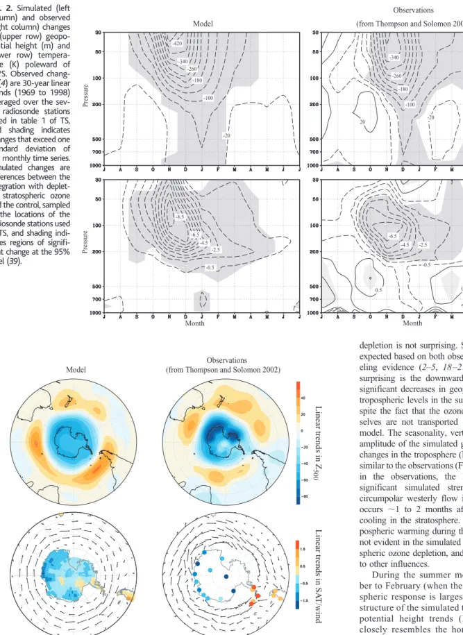
In the stratosphere, the prescribed ozone depletion induces cooling over the polar cap as a result of reduced absorption of ultraviolet radiation (Fig. 2, bottom left). Consistent with observations (4,5,18), the response is largest when sunlight returns to the polar region in November, and it persists through the summer months. The simulated stratospheric cooling is accompanied by a strengthening of the strato- spheric circumpolar flow that also peaks during November (Fig. 2, top left) and is consistent with the observed increased persistence of the stratospheric vortex (2–5). During the spring and summer months, both the vertical structure and the amplitude of the simulated stratospheric geopotential height and temperature trends are similar to the observations presented in TS (Fig.
2, right panels). The most pronounced differ- ence between the observed and simulated stratospheric trends occurs during April and May, when the observations exhibit a pro- nounced decrease in geopotential height, which is not simulated by the model.
The simulation of a large response in the extratropical stratosphere to prescribed ozone
1School of Earth and Ocean Sciences, University of Victoria, Post Office Box 3055, Victoria, BC V8W3P6, Canada.2Department of Atmospheric Science, Foot- hills Campus, Colorado State University, Fort Collins, CO 80523, USA.
*To whom correspondence should be addressed. E-
mail: gillett@uvic.ca Month
Pressure
-20%
0 -40%
-60%
-80%
Prescribed ozone losses (%) Fig. 1. Prescribed change in ozone plotted as a function of month and pressure at 70°S, based on observed ozone trends from 1979 to 1997 (16).
R
E P O R T Swww.sciencemag.org SCIENCE VOL 302 10 OCTOBER 2003
273
depletion is not surprising. Such a response is expected based on both observations and mod- eling evidence (2–5, 18 –21). What is more surprising is the downward extension of the significant decreases in geopotential height to tropospheric levels in the summer months, de- spite the fact that the ozone anomalies them- selves are not transported downward by the model. The seasonality, vertical structure, and amplitude of the simulated geopotential height changes in the troposphere (Fig. 2, top left) are similar to the observations (Fig. 2, top right). As in the observations, the largest and most significant simulated strengthening of the circumpolar westerly flow in the troposphere occurs ⬃1 to 2 months after the maximum cooling in the stratosphere. The observed tro- pospheric warming during the other seasons is not evident in the simulated response to strato- spheric ozone depletion, and thus is likely due to other influences.
During the summer months of Decem- ber to February (when the simulated tropo- spheric response is largest), the horizontal structure of the simulated tropospheric geo- potential height trends (Fig. 3, top left) closely resembles the horizontal structure of the observed trends shown in TS (Fig. 3, top right). Both reveal falling geopotential heights poleward of 60°S and rising geopo- tential heights in the middle latitudes (22).
In both the observations and the model, the trends in the 500-hPa height field strongly resemble the structure of the SAM. Consis-
30-yr linear trends in Z
Month
30-yr linear trends in T
Pressure
-20 -260
-100
-100
20 -180
-340
20
-2.5
-0.5 -4.5 -6.5
0.5 0.5 -20
-260
-100 -420
-180 -340
Month
Pressure -2.5
-0.5 -4.5 -6.5 -8.5
Model
Observations
(from Thompson and Solomon 2002) Fig. 2. Simulated (left
column) and observed (right column) changes in (upper row) geopo- tential height (m) and (lower row) tempera- ture (K) poleward of 65°S. Observed chang- es (4) are 30-year linear trends (1969 to 1998) averaged over the sev- en radiosonde stations listed in table 1 of TS, and shading indicates changes that exceed one standard deviation of the monthly time series.
Simulated changes are differences between the integration with deplet- ed stratospheric ozone and the control, sampled at the locations of the radiosonde stations used in TS, and shading indi- cates regions of signifi- cant change at the 95%
level (39).
Linear trends in Z500Linear trends in SAT/wind Observations
Model (from Thompson and Solomon 2002)
Fig. 3.Simulated (left column) and observed (right column) changes in (upper row) 500-hPa geopotential height (m) and (lower row) near-surface temperature (K) and winds. Observed changes (4) are 22-year linear trends in 500-hPa geopotential height and 925-hPa winds (1979 to 2000), and 32-year linear trends in surface temperature (1969 to 2000) averaged over December to May (22). Simulated changes are differences between the perturbed and control integrations in 500-hPa geopotential height, 950-hPa winds, and land surface temperature averaged over December to February. The longest wind vector corresponds to⬃4 m/s.
R
E P O R T S10 OCTOBER 2003 VOL 302 SCIENCE www.sciencemag.org
274
tent with the dynamics associated with a shift toward the positive polarity of the SAM (23–26), the simulated tropospheric trends are accompanied by increases in the poleward eddy flux of momentum across
⬃50°S (not shown). Hence, the simulated trends in the tropospheric circulation are reinforced by the attendant changes in tro- pospheric eddy activity. The details of the mechanisms whereby stratospheric anoma- lies influence the circulation of the tropo- sphere are still under investigation (27).
The simulated trend in the SAM during the summer months is accompanied by a significant surface cooling over most of Ant- arctica (28) and by a strengthening of the surface westerly flow at around 50°S to 60°S (Fig. 3, bottom left), also consistent with the observations (Fig. 3, bottom right). The cool- ing within the region of enhanced tropospher- ic westerlies is consistent with adiabatic changes in temperature driven by thermally indirect rising motion there (4,24). However, radiative cooling due to decreased down- welling longwave radiation may also have played a role in cooling the polar troposphere (29). The relatively weak warming over the Antarctic Peninsula and Patagonia is also consistent with the observations and likely reflects the impact of temperature advection by the anomalous westerly flow streaming from the relatively warm waters west of the Drake Passage. Consistent with the hemi- spheric scale structure of the SAM (6), both the simulated and observed trends in the near- surface flow contain easterly anomalies at around 30°S, with changes of up to⬃1 m/s to the east of Australia and across the southern Atlantic and Indian Oceans (Fig. 4).
Several factors have been proposed as capable of driving a trend in the SAM.
Simulations run with increasing greenhouse gases reveal trends in the SAM that are of the same sign as the observed trends (12, 30,31), but the amplitude of the simulated trends is considerably smaller than that ob- served. At least one study has suggested that increases in tropical sea-surface tem- peratures have played a role in driving analogous trends in the Northern Hemi-
sphere (32), but to what extent these results apply to the SAM remains to be demonstrated.
The results reported in this study support the hypothesis outlined in TS that photochemical ozone depletion has played a critical role in driving recent climate change not only in the SH stratosphere but in the SH troposphere as well. Both the “downward propagation” of the simulated circulation anomalies during the spring months and the vertical and horizontal structure of the simulated trends during the summer months bear a striking resemblance to observations of recent SH climate change. The discrepancy between the simulated and ob- served trends during the months of April and May implies that the observed trends during this season are not attributable to the prescribed ozone depletion.
The results in this study add to an in- creasing body of both observational (7,33, 34) and modeling (35, 36) evidence that suggests stratospheric processes play an important role in driving climate variability at the surface of the Earth on a range of time scales, particularly at high latitudes.
Taken together with the observations pre- sented in TS, the findings reported here strongly suggest that human emissions of ozone-depleting gases have demonstra- bly affected surface climate over the past few decades.
References and Notes
1. J. W. Hurrell, H. van Loon,Tellus46A, 325 (1994).
2. D. W. Waugh, W. J. Randel, S. Pawson, P. A. Newman, E. R. Nash,J. Geophys. Res.104, 27191 (1999).
3. S. T. Zhou, M. E. Gelman, A. J. Miller, J. P. McCormack, Geophys. Res. Lett.27, 1123 (2000).
4. D. W. J. Thompson, S. Solomon, Science296, 895 (2002).
5. W. J. Randel, F. Wu,J. Clim.12, 1467 (1999).
6. The structure of the SAM is discussed in, for example, (23), (24), (37), and (38).
7. D. W. J. Thompson, M. P. Baldwin, S. Solomon, in preparation.
8. A similar lag has also been observed between the stratospheric and tropospheric circulations in the Northern Hemisphere (33,34).
9. D. G. Vaughan, G. J. Marshall, W. M. Connolley, J. C.
King, R. Mulvaney,Science293, 1777 (2001).
10. D. M. H. Sexton,Geophys. Res. Lett.28, 3697 (2001).
11. I. T. Kindem, B. Christiansen,Geophys. Res. Lett.28, 1547 (2001).
12. N. P. Gillett, M. R. Allen, K. D. Williams, Q. J. R.
Meteorol. Soc.129, 947 (2003).
13. The prescribed ozone losses used in (12) are as much as two times as large as the observed estimates presented in (16) during certain seasons.
14. As noted in (12), the response of HadSM3 to strato- spheric ozone depletion is sensitive to the vertical resolution below 10 hPa. Hence, the 19-level version of the model used in (10) yields a weaker response than that used in this study.
15. D. M. Li, K. P. Shine, “A 4-dimensional ozone clima- tology for UGAMP models,”Internal Rep. 35, UK Universities Global Atmospheric Modelling Pro- gramme (1995).
16. W. J. Randel, F. Wu,Geophys. Res. Lett. 26, 3089 (1999).
17. Both the control and the perturbed simulations were integrated for 30 years. Equilibrium was reached after 11 years in the control simulation and after 5 years in the perturbed simulation.
18. V. Ramaswamyet al.,Rev. Geophys.39, 71 (2001).
19. K. P. Shine,Geophys. Res. Lett.13, 1331 (1986).
20. J. T. Kiehl, B. A. Boville,J. Atmos. Sci.45, 1798 (1988).
21. J. D. Mahlman, J. P. Pinto, L. J. Umscheid,J. Atmos. Sci.
51, 489 (1994).
22. The observed trends presented in Fig. 3 are based on the months December to May, because they are reproduced from TS. The simulated results presented in Fig. 3 are based on the months December to February, because the model does not reproduce the observed trends during April and May. In practice, the observed trends for the limited season December to February are similar to those presented in Fig. 3.
23. D. L. Hartmann, F. Lo,J. Atmos. Sci.55, 1303 (1998).
24. D. W. J. Thompson, J. M. Wallace,J. Clim.13, 1000 (2000).
25. D. J. Lorenz, D. L. Hartmann,J. Atmos. Sci.58, 3312 (2001).
26. V. Limpasuvan, D. L. Hartmann,J. Clim.13, 4414 (2000).
27. M. P. Baldwin, D. W. J. Thompson, E. F. Shuckburgh, W. A. Norton, N. P. Gillett,Science301, 317 (2003).
28. The 0.46-K simulated surface cooling averaged over Antarctica is significant at the 95% level based on the tstatistic.
29. M. Lal, A. K. Jain, M. C. Sinha,Tellus39B, 326 (1987).
30. J. C. Fyfe, G. J. Boer, G. M. Flato,Geophys. Res. Lett.
26, 1601 (1999).
31. P. J. Kushner, I. M. Held, T. L. Delworth,J. Clim.14, 2238 (2001).
32. M. P. Hoerling, J. W. Hurrell, T. Y. Xu,Science292, 90 (2001).
33. M. P. Baldwin, T. J. Dunkerton,J. Geophys. Res.104, 30937 (1999).
34. M. P. Baldwin, T. J. Dunkerton, Science 294, 581 (2001).
35. B. A. Boville,J. Atmos. Sci.41, 1132 (1984).
36. L. M. Polvani, P. J. Kushner,Geophys. Res. Lett.29, 10.1029/2001GL014284 (2002).
37. J. W. Kidson,J. Clim.1, 1177 (1988).
38. D. J. Karoly,Tellus42A, 41 (1990).
39. The significance of the differences in means between experiments was assessed at the 95% level using a two-samplettest.
40. E. Kalnayet al.,Bull. Am. Meteorol. Soc.77, 437 (1996).
41. We thank S. Solomon and J. Arblaster for discussion of the results; D. Karoly and two anonymous review- ers for their insightful comments; L. Donner, W.
Randel, and P. Kushner for helpful suggestions and comments on an earlier version of the manuscript;
and A. Iwi, J. Kettleborough, and M. Palmer for help running the model. The model integrations were funded under the Upper Troposphere Lower Strato- sphere Ozone program of the UK Natural Environ- ment Research Council, ref. NERC/T/S/2000/00114.
N.P.G. is supported in Victoria by Canadian Climate Variability Research Network funding from the Nat- ural Sciences and Engineering Research Council of Canada and the Canadian Foundation for Climate and Atmospheric Sciences. D.W.J.T. is supported by the NSF under grants CAREER:ATM-0132190 and ATM- 0320959.
30 May 2003; accepted 26 August 2003 Model
Observations Fig. 4.Simulated (up-
per panel) and ob- served (lower panel) changes in near-sur- face winds, as shown in Fig. 3, but for the SH low–middle lati- tudes. The observed trends are calculated as in TS Fig. 2 using data described in (40).
R
E P O R T Swww.sciencemag.org SCIENCE VOL 302 10 OCTOBER 2003