Multivariate Association
Theory and Applications to Financial Data
Inauguraldissertation zur
Erlangung des Doktorgrades der
Wirtschafts- und Sozialwissenschaftlichen Fakult¨at der
Universit¨at zu K¨oln
2010
vorgelegt von
Dipl.-Math. oec., MSc Sandra Caterina Gaißer aus
Stuttgart
Referent: Prof. Dr. Friedrich Schmid, Universit¨at zu K¨oln Korreferent: Prof. Dr. Karl Mosler, Universit¨at zu K¨oln Tag der Promotion: 17. Dezember 2010
I would like to thank Professor Friedrich Schmid for giving me the opportunity to pursue this doctorate at the Department of Economic and Social Statistics at the University of Cologne. I am deeply grateful for his excellent guidance and supervision and the stimulating research environment during the entire phase of my doctoral work.
I am also indebted to Professor Karl Mosler for his willingness to act as a referee of my dissertation. I would like to thank him for his support and helpful comments.
Further, I would like to thank Professor Eckart Bomsdorf for his advice and many fruitful discussions.
My special gratitude belongs to Dr. Christoph Memmel and Dr. Carsten Wehn for giving me the opportunity for a joint research project at the Banking and Financial Supervision Department at the Deutsche Bundesbank. Various theoretical results of this thesis have been inspired by the practical questions and problems from risk mea- surement and management revealed during this project. I would also like to thank Dr.
Thilo Liebig and the Deutsche Bundesbank for making this collaboration possible and for the financial support.
Moreover, I am very thankful to Professor Ragnar Norberg who introduced me to the world of academic research during my time at the Department of Statistics at the London School of Economics. He filled me with enthusiasm in many fields of actuarial, financial and statistical sciences. Further, I am indebted to Dr. Jeremy Penzer for his guidance during my studies at the aforementioned department.
I am also very grateful to Professor R¨udiger Kiesel and Professor Hans-Joachim Zwiesler and many others at the Faculty of Mathematics and Economics at the Uni- versity of Ulm. The foundation for my academic knowledge and interest has been laid during my studies there. In particular, I would like to mention the excellent supervision and guidance of Professor R¨udiger Kiesel.
Many thanks also to my colleagues and friends at the University of Cologne for their support and many helpful discussions. I would like to name Dr. Oliver Grothe, PD Dr.
Gabriel Frahm, Thomas Blumentritt, Carsten K¨orner, Michael Stegh, Dr. Bernhard Babel, Michel Becker-Peth, and Leila Samad-Tari. Moreover, I would like to thank my colleague Martin Ruppert for the successful research collaboration.
Finally, I am very much indebted to Rafael, my parents and the rest of my family for supporting, motivating and encouraging me during all stages of my life.
Sandra Gaißer
K¨oln, 10th December 2010
1 Introduction 7 2 Statistical modeling and measurement of association 15
2.1 Association in financial data . . . 15
2.2 Modeling multivariate association - the concept of copulas . . . 20
2.2.1 Definition, properties, and examples . . . 20
2.2.2 Statistical inference: The empirical copula (process) . . . 25
2.3 Measuring multivariate association . . . 37
2.3.1 Concordance, positive dependence, and comonotonicity . . . 37
2.3.2 Properties of measures of multivariate association . . . 39
2.3.3 Spearman’s rho, Kendall’s tau, and Blomqvist’s beta . . . 41
3 A multivariate version of Hoeffding’s Phi-Square 47 3.1 Preliminaries . . . 47
3.2 Multivariate Hoeffding’s Phi-Square . . . 48
3.3 Statistical inference for multivariate Hoeffding’s Phi-Square . . . 53
3.3.1 Nonparametric estimation . . . 54
3.3.2 Small sample adjustments . . . 60
3.4 Empirical study . . . 64
3.5 Calculations and proofs . . . 66
3.5.1 Derivation of the functionsh(d)−1 andg(d)−1 . . . 66
3.5.2 Derivation of the estimator Φb2n . . . 67
3.5.3 Proofs . . . 68
4 Estimating multivariate association based on weighted observations 71 4.1 Preliminaries . . . 71
4.2 Multivariate weighted Spearman’s rho . . . 73
4.2.1 Weighted nonparametric estimation . . . 73
4.2.2 Asymptotic behavior . . . 74
4.3 Time-dynamic weighted Spearman’s rho . . . 85
4.4 Empirical study . . . 91
4.5 Appendix . . . 96
5 Testing equality of pairwise rank correlations in a multivariate ran- dom vector 97 5.1 Preliminaries . . . 97
5.2 Statistical tests for equi rank-correlation . . . 100
5.2.1 Test statistics Tn,1 andTn,2 . . . 100
5.2.2 Test statistics Tn,3 andTn,4 . . . 106
5.3 Classical tests for equi linear-correlation . . . 109
5.4 Simulation study . . . 110
5.4.1 Modeling the set of alternative hypothesis . . . 110
5.4.2 Simulation results . . . 112
5.5 A test for stochastic independence . . . 115
5.6 Empirical study . . . 116
5.7 Appendix . . . 118
5.7.1 Rank correlation coefficient ρ . . . 118
5.7.2 Simulation results referring to the estimation of the asymptotic covariance matrix . . . 119
6 Time dynamic and hierarchical dependence modeling of a supervisory portfolio of banks 123 6.1 Motivation . . . 123
6.2 Control charts . . . 125
6.3 Time-dynamic and hierarchical testing for long-term level changes of Spearman’s rho . . . 127
6.3.1 Detecting long-term level changes of Spearman’s rho over time . 135 6.3.2 Hierarchical testing . . . 137
6.4 The standardized profits and losses of the supervisory portfolio . . . 139
6.5 Empirical results . . . 140
6.5.1 Standardized returns . . . 141
6.5.2 Multivariate Spearman’s rho of the supervisory portfolio . . . 142
6.5.3 Level changes of Spearman’s rho of the supervisory portfolio over time . . . 144
6.5.4 Hierarchical considerations for the supervisory portfolio . . . 146
Bibliography 151
List of Tables 161
List of Figures 165
Index 168
Abbreviations
U(0,1) continuous uniform distribution with support [0,1] . . . 22
N(µ, σ2) univariate normal distribution . . . 43
N(µ,Σ) multivariate normal distribution . . . 99
χ2m univariate χ2-distribution with m degrees of freedom . . . 101
Φ distribution function of the univariate standard normal distribution 24 tv distribution function of the univariate t-distribution with ν degrees of freedom . . . 24
Γ(·) Gamma function . . . 66
l∞([0,1]d) space of uniformly bounded, real functions on [0,1]d . . . 27
C([0,1]d) space of continuous functions on [0,1]d. . . 29
D([0,1]d) space of cadlag functions on [0,1]d. . . 29
IN natural numbers . . . 86
Z integer numbers . . . 35
IR real numbers . . . 26
IR¯ extended real numbers, [∞,∞] . . . 29
IRd d-dimensional real space . . . 21
C copula function C: [0,1]d→ [0,1] . . . 20
C˘ survival copula . . . 22
G survival function of a distribution functionG . . . 22
G−1 generalized inverse of a distribution functionG . . . 21
G,B Gaussian processes . . . 28
RanX range of random variableX . . . 23
β(X) strictly monotone transformation ofX. . . 23
δ measure of association . . . 39
αX mixing coefficient associated with sequence{Xj}j∈Z of multivariate random vectors . . . 35
∨ maximum . . . 31
∧ minimum . . . 28
≺ concordance ordering . . . 37
−→w weak convergence . . . 31
−→d convergence in distribution . . . 43
−→IP convergence in probability . . . 106
EWMA exponentially weighted moving average . . . 10
SE standard error . . . 96
VaR Value-at-Risk . . . 124
P&L (trading) profits and losses . . . 124
E(X) expectation of random variableX. . . 53
V ar(X) variance of random variableX. . . 41
Cov(X, Y) covariance of random variablesX, Y . . . 41
Introduction
Concepts of association or dependence play a central role when considering multiple random sources in statistical models as they describe the relationship between two or more random variables. Several questions are of relevance in this context:
1. How can association be measured and detected in empirical data?
2. How can association between random variables be modeled in general?
3. Which estimation and statistical test procedures are available?
Especially in financial applications, the analysis and modeling of association has gained a lot of attention recently and is subject to an increasing research activity. We mention multivariate portfolio theory, risk analysis and management, valuation, hedging, and pricing of complex financial instruments such as basket default options. In particular, the concept of copulas has proven to be useful in those fields of application and re- search. Before going into detail as far as the modeling and measurement of association by means of copulas is concerned, we briefly describe the role of association within some of the aforementioned fields.
Within portfolio theory, prominent concepts such as the Mean-Variance Markowitz model (Markowitz (1987)), the Capital Asset Pricing Model (CAPM), and the Ar- bitrage Pricing Theory (APT) (see e.g. Elton et al. (2010)) make use of Pearson’s correlation coefficient as a measure of association between the asset returns in order to determine an optimal portfolio choice for a given utility function. In this context, Pearson’s correlation coefficient has proven to be a tractable measure while offering an appealing way to describe association between multivariate normally distributed asset returns. The latter distributional assumption, however, is essential for the applicabil- ity of Pearson’s correlation coefficient as a measure of association, as we will explain below. Pearson’s correlation coefficient is also frequently used in the context of risk measurement and management of multivariate asset portfolios. This can partly be put down to the fact that the common risk measure Value-at-Risk (VaR) may be expressed as a simple function of the correlation matrix of the multivariate normally distributed
asset returns in the underlying portfolio, representing a coherent risk measure in this case. In particular, the one-factor portfolio model proposed in Pillar I of the regulatory Basel II framework (cf. Basel Committee on Banking Supervision (2006)) makes use of an elegant relationship between the correlation structure of the underlying portfolio and the VaR. We further recall the widely used methodology by RiskMetrics (1996) for measuring market risk, which is based on the assumption of normally distributed returns and the VaR concept. In particular, weighted averages of past observations are used here to forecast and estimate volatility and correlation.
Many researchers and practitioners have extended the above and many other appli- cations to more general concepts of association than Pearson’s correlation coefficient.
The reasons for those extensions are numerous. For example, Pearson’s correlation coefficient is known to be sensitive towards extreme events and, thus, more robust measures of association such as trimmed correlation coefficients have been suggested (see e.g. Maronna et al. (2006)). Further, Pearson’s correlation coefficient measures the degree of linear association between two random variables. Usually, however, this does not sufficiently describe association between non-normally or, more generally, non- elliptically distributed random variables (related pitfalls are discussed in Embrechts et al. (2002)). In particular, the concept of correlation does not exist for very heavy-tailed distributions such as alpha-stable distributions where the second moments do not ex- ist (see e.g. Rachev and Mittnik (2000)). In addition, we mention complex non-linear financial products such as basket default options where the correlation coefficient as a second-order approximation to association represents a less adequate measure (cf.
Laurent and Gregory (2005) and references therein). Another extension of the cor- relation coefficient, which measures association between two random variables only, refers to the simultaneous measurement of association between more than two random variables as described by their multivariate distribution function. This type of multi- variate measures of association will be developed and investigated in the present thesis.
Amongst those various extensions, the concept of copulas has proven to be the most general and sophisticated concept of describing and modeling association or dependence between the components of a random vector (see e.g. Joe (1997) and Nelsen (2006) for a detailed overview of copulas). Copula techniques are also frequently applied in the quantitative finance literature, we mention Patton (2002), Embrechts et al. (2003), McNeil et al. (2005), Savu and Trede (2008), and Giacomini et al. (2009). Copulas split the multivariate distribution function of a random vector into the univariate marginal distribution functions and the dependence structure represented by the copula. In particular, the copula is invariant with respect to strictly increasing transformations of the components of the random vector. Commonly, it is precisely this property which justifies to call the copula the dependence structure of a random vector. Naturally, measures of association or dependence should be a functional of the copula only. The most prominent measures of this type are Spearman’s rho and Kendall’s tau. Especially the former measure will be the subject of several analyses and results in this thesis.
Outline and summary
The main aim of this dissertation is the modeling, the estimation and the statisti- cal inference of multivariate versions of copula-based measures of association such as Spearman’s rho. Special focus is put on the analysis of the statistical properties of related estimators as well as the derivation of statistical hypothesis tests. The latter may be used to verify specific modeling assumptions on the one hand. On the other hand, statistical tests are developed to test whether association changes over time or whether it differs between random sources such as multivariate asset returns. Only a few statistical tests of those types exist for multivariate measures of association in the copula framework. This thesis addresses this gap and illustrates the theoretical results with applications to financial data. Further, several simulation studies are carried out to investigate the performance of the proposed estimators or statistical hypothesis tests.
All theoretical results in this thesis on the modeling and measuring of association between several random variables use the concept of copulas. In fact, copulas allow to study the dependence structure of a multivariate random vector irrespective of its univariate marginal distribution functions. We consider measures of association which depend on the copula of the underlying random vector only and are invariant with re- spect to the marginal distribution functions. As a direct functional of the copula, non- parametric estimators for those measures are obtained based on the so called empirical copula, which is derived from the multivariate empirical distribution function. Statis- tical inference for these measures is established using recent results on the asymptotic weak convergence of the empirical copula process, also for serially dependent observa- tions. The derived results and hypothesis tests are mainly of nonparametric nature and may thus be applied in very general settings. Only weak assumptions on the distribu- tion function, such as continuity of the marginal distributions and continuous partial differentiability of the copula, are made.
One aspect in this thesis is the measurement of multivariate association. As out- lined above, measures of multivariate association are naturally based on the copula of the underlying random vector. Various copula-based measures have been proposed in the literature. For example, Wolff (1980) introduces a class of multivariate measures of association which is based on the L1- andL∞-norms of the difference between the cop- ula and the independence copula (see also Fern´andez-Fern´andez and Gonz´alez-Barrios (2004)). Other authors generalize existing bivariate measures of association to the mul- tivariate case. For example, multivariate extensions of Spearman’s rho are considered by Nelsen (1996) and Schmid and Schmidt (2006, 2007a, 2007b). Blomqvist’s beta is generalized by ´Ubeda-Flores (2005) and Schmid and Schmidt (2007c), whereas a mul- tivariate version of Gini’s Gamma is proposed by Behboodian et al. (2007). Further, Joe (1990) and Nelsen (1996) discuss multivariate generalizations of Kendall’s tau. A multivariate version of Spearman’s footrule is considered by Genest et al. (2010). Joe (1989a, 1989b) investigates multivariate measures which are based on the Kullback- Leibler mutual information. Most of these measures have the often undesirable prop- erty that they may be zero even though the components of the underlying random
vector are not stochastically independent. In chapter 3 of this thesis, we propose a multivariate version of the bivariate measure Hoeffding’s Phi-Square which takes the value zero if and only if the components of the random vector are stochastically in- dependent. It is based on a Cram´er-von Mises functional and is of importance in the context of tests for (multivariate) stochastic independence. In particular, it is a direct functional of the copula only. The asymptotic distribution of a nonparametric estima- tor for Hoeffding’s Phi-Square is established for the case of independent observations as well as of dependent observations from a strictly stationary strong mixing sequence.
Another important topic of this thesis is the derivation of a weighted version for Spearman’s rho, which is addressed in chapter 4. A shared feature of such weighted statistics is to allocate different, non-identical weights to the observations. In a time- dynamic context, for example, different weights are put on past observations to model the evolving correlation over time. A popular representative of this type of weighted statistics is the Exponentially Weighted Moving Average (EWMA) model, introduced by RiskMetrics (1996). Based on observationsXt−n+1, ...XtandYt−n+1, . . . , Yt,respec- tively, the estimator for the (linear) correlation at time tis here given by
rt=
Pn
j=1λj−1(Xt−j+1−X)(Y¯ t−j+1−Y¯) qPn
j=1λj−1(Xt−j+1−X)¯ 2qPn
j=1λj−1(Yt−j+1−Y¯)2
(1.1)
with ¯X = 1/nPn
i=jXt−j+1and ¯Y = 1/nPn
j=1Yt−j+1and decay factor 0< λ <1.The decay factorλdetermines the relative weight which is assigned to each observation. In contrast to a simple moving average model based on equally weighted observations (i.e., withλ= 1), the above estimator reacts faster to (sudden) changes of the correlation as higher weight is allocated to more recent observations. The RiskMetrics methodology is based on the assumption that the underlying multivariate distribution is (condition- ally) normally distributed. As outlined above, other concepts of association than linear correlation are more appropriate when the underlying distributions are non-elliptical.
This motivates the introduction of a weighted estimator for the copula-based measure Spearman’s rho. As the estimation of Spearman’s rho is based on the ranks of the observations, the proposed weighted estimator places different weights to the ranks of the observations and not to the observations themselves, as e.g. in the EWMA model.
The asymptotic distribution of this estimator is derived from the weak convergence of weighted empirical processes. Those results allow, for example, to test for significant changes of Spearman’s rho over time. A generalization to the multivariate case is also considered.
An assumption frequently made in many financial and statistical models is that pairwise correlations between the underlying random variables are equal. For exam- ple, the one-factor portfolio model used in the Basel II framework (BCBS (2006)), which determines the minimum capital requirements for credit risk, is based on the assumption that the asset returns between any two obligors have the same correlation.
Engle and Kelly (2009) consider equal pairwise correlations in the context of dynamic conditional correlation modeling. They describe further applications in collateralized
debt obligation (CDO) pricing, derivative trading, and portfolio choice. Another field of research where the assumption of equal pairwise correlations plays a central role is the interclass correlation modeling, which is applied within the analysis of familial data. The latter investigates the degree of resemblance between family members and is subject to increasing research activity, see e.g. Helu and Naik (2006), Seo et al. (2006), Naik and Helu (2007), and Wu et al. (2009) and references therein. The assumption of equal pairwise correlations can be verified utilizing adequate statistical tests. Various tests for the null hypothesis of equal linear Pearson’s correlation coefficients (or equi linear-correlation) in a multivariate normally distributed random vector have been in- vestigated e.g. by Bartlett (1950, 1951), Anderson (1963), Lawley (1963), and Aitkin et al. (1968). Due to the aforementioned shortcomings of Pearson’s correlation coef- ficient, it is natural to study alternative measures of association such as Spearman’s rho. In chapter 5, we develop four (asymptotic) tests for the null hypothesis of equi Spearman’s rank-correlation, i.e., that all pairwise Spearman’s rho coefficients in a multivariate random vector are equal. The proposed tests for equi rank-correlation are nonparametric and can be applied without further assumptions on the marginal distributions except their continuity. As demonstrated, the proposed tests may also be applied in the context of multivariate distribution modeling. All tests are easy to implement and can be performed with low computational complexity. A simulation study to investigate the power of the tests identifies especially two tests showing a good performance for all considered dimensions and copula models. The test setting also allows the derivation of a test for stochastic independence based on all distinct pairwise Spearman’s rho coefficients.
As mentioned before, the analysis of the association in a portfolio of risky assets has attracted increasing interest over the last decade. First, the globalizing and interdepen- dence of financial markets require a thorough portfolio risk modeling and management, which can quickly react to changing market situations. This is particularly important when market conditions deteriorate and the association between asset returns increases – which is also known as the ‘correlation breakdown’, see e.g. Karolyi and Stulz (1996), Campbell et al. (2002), Bae et al. (2003), Patel (2005), Rodriguez (2007) or Bartram et al. (2007). Simultaneously, the rising awareness of modeling the association in a portfolio may certainly be put down to the recent market turbulence in the entire fi- nancial sector. Further, the internal model approach in the context of the regulatory Basel II framework allows banks to use their own portfolio risk models for determining the amount of regulatory capital to be maintained. Hence, a proper understanding of the portfolio’s cross correlation structure and diversification may be essential to preserve the financial stability of a bank on the one hand. On the other hand, increas- ing association between financial asset returns may also lead to increasing association between banks’ trading results and, thus, to the risk of simultaneous large losses at several banks. A comprehensive analysis of the association between the banks’ trading results may give information about the systemic fragility of the financial system. From a supervisory perspective, we develop two test procedures in chapter 6 to analyze the association between the trading results of a hypothetical portfolio of banks both over time and across banks. In particular, we use Spearman’s rho to quantify the association
in this supervisory portfolio. Several theoretical results on the asymptotic behavior of the difference of two Spearman’s rho coefficients - either between two different samples or for different points in time - form the basis for the formulation of the two test proce- dures. On the one hand, a time-dynamic two-step test procedure, which is partly based on a nonparametric control chart for Spearman’s rho, is designed to detect significant long-term level changes of Spearman’s rho. On the other hand, we propose a statistical hypothesis test for significant differences between two Spearman’s rho coefficients of different samples by taking into account all respective lower-dimensional Spearman’s rho coefficients. This test can be used to simultaneously identify those groups of banks that show significant changes of association around some specific point in time. The theoretical results are applied to real profits and loss data and corresponding Value- at-Risk estimates of eleven German banks which had a regulatory approved internal market-risk model during the years 2001 to 2006. Our empirical study of the super- visory portfolio identifies significant changes in the level of Spearman’s rho at three time points during the observation period. At two of those time points the second test procedure reveals a significant change in association for all sub-portfolios comprising more than eight banks. The proposed methods are general and can be applied to any series of multivariate asset returns in finance where the assumption of independent standardized returns holds.
Detailed outline
Chapter 2 deals with the statistical modeling and measurement of multivariate as- sociation. We start by describing several properties of association in financial data by introducing different statistical tools and concepts to measure and detect associa- tion. The concept of copulas is introduced in section 2.2.1 and several properties of copulas are presented. In section 2.2.2, we discuss the nonparametric estimation of copulas based on the empirical copula. The weak convergence of the empirical copula process is investigated for both independent and serially dependent observations from strictly stationary strong mixing sequences. We further give a brief introduction to the nonparametric bootstrap which can be used to approximate the distribution of the empirical copula process. After introducing several concepts of multivariate associa- tion such as concordance or positive dependence in section 2.3.1, section 2.3.2 discusses important properties of multivariate measures of association. Finally, we introduce the (bivariate) copula-based measures of association Spearman’s rho, Kendall’s tau, and Blomqvist’s beta, describe how they can be generalized to the multivariate case, and address their estimation based on the empirical copula in section 2.3.3.
A multivariate version of the measure of association Hoeffding’s Phi-Square is dis- cussed in chapter 3. Some of its analytical properties are investigated in section 3.2. We give the explicit value of multivariate Hoeffding’s Phi-Square for some copulas of simple form and describe a simulation algorithm to approximate its value when the copula is of a more complicated form. In section 3.3, a nonparametric estimator for multivari- ate Hoeffding’s Phi-Square based on the empirical copula is derived. We establish its
asymptotic behavior both in the case of independent observations and dependent ob- servations from strictly stationary strong mixing sequences. The asymptotic variance can consistently be estimated by means of a nonparametric (moving block) bootstrap method. We show how the estimator can be adapted to account for small sample sizes.
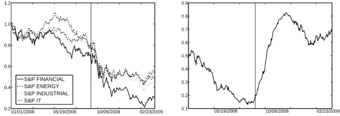
Section 3.4 finally illustrates the applicability of multivariate Hoeffding’s Phi-Square to financial data by using it to analyze financial contagion related to the bankruptcy of Lehman Brothers Inc. in September 2008.
In chapter 4, a weighted nonparametric estimator for multivariate Spearman’s rho is proposed and its statistical properties are investigated. After providing relevant definitions and background material in section 4.1, the weighted estimator for multi- variate Spearman’s rho is introduced in section 4.2. It is derived from the ordinary nonparametric estimator of Spearman’s rho based on the empirical copula by allocat- ing nonidentical weights to the ranks (section 4.2.1). In section 4.2.2, we first establish the weak convergence of the weighted empirical copula process under minimal condi- tions on the weights, which is deduced from the weak convergence properties of general weighted empirical processes. In a second step, the asymptotic behavior of the weighted estimator for Spearman’s rho is derived. A bootstrap procedure is described to esti- mate the asymptotic variance of this estimator. Section 4.3 deals with the application of the weighted estimator for evaluating Spearman’s rho over time while placing more weight to recent observations. Several weighting schemes for this purpose are discussed.
Finally, the theoretical results are applied to the analysis of association between equity return series of several international banks in section 4.4.
Chapter 5 addresses the statistical testing of the null hypothesis of equi-rank cor- relation, i.e., that all pairwise Spearman’s rho coefficients in a multivariate random vector are equal. After providing relevant definitions and some preliminary results on Spearman’s rho in section 5.1, four (asymptotic) nonparametric hypothesis tests for equi rank-correlation are derived in section 5.2. We establish their asymptotic distri- bution based on empirical process theory. We show that a nonparametric bootstrap method to determine unknown parameters or critical values works. Further, a brief overview of the existing literature on tests for equi linear-correlation is given in section 5.3. The results of a simulation study carried out to investigate the power of the tests are discussed in section 5.4. They are compared to the classical test for equal linear Pearson’s correlation coefficients developed by Lawley (1963). Section 5.5 briefly dis- cusses the derivation of a test for stochastic independence based on Spearman’s rho before the applicability of the four tests for equi-rank correlation to financial data is demonstrated in section 5.6.
Finally, the last chapter of this thesis, chapter 6, is devoted to the statistical analysis of association in a supervisory portfolio of banks both over time and across banks. After a short motivation in section 6.1, an introduction to the basic theory of control charts is given in section 6.2. The relevant theoretical results on the difference of two Spearman’s rho coefficients both over time and across different samples are established in section
6.3. In particular, the test procedure for detecting significant long-term level changes of Spearman’s rho is developed in section 6.3.1. The statistical test procedure designed to analyze the statistical properties of multiple Spearman’s rho coefficients is derived in 6.3.2. Section 6.4 states relevant definitions and assumptions for the analysis of the supervisory portfolio. The theoretical findings are applied to real profits and loss data and corresponding Value-at-Risk estimates of eleven German banks in section 6.5.
Statistical modeling and
measurement of association
2.1 Association in financial data
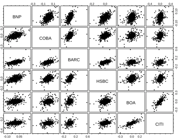
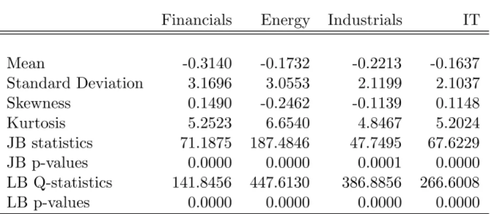
As outlined in the previous chapter, the notion of association plays a central role in many applications in financial theory. In the following, we describe some aspects of detecting and measuring association in financial data by using different statistical con- cepts. Throughout this section, our analysis is based on daily equity (log-) return series from the six international banks BNP Paribas (BNP), Commerzbank (COBA), Bar- clays (BARC), HSBC, Bank of America (BOA), and Citigroup (CITI) from May 1997 to April 2010.
Figure 2.1 shows a scatter plot matrix for the return series of all pairs of banks.
The distinct scatter plots give a first impression of the degree and type of association between the return series. In particular, they show that association in financial data is quite different. This observation is confirmed by figure 2.2, which provides contour plots of the empirical densities of two selected pairs of banks. Whereas the level curves of the empirical density in the right panel of figure 2.2 are rather elliptic, the level curves in the left panel have a quite different shape.
The most common measure to quantify the degree of association between two ran- dom variables is Pearson’s linear correlation coefficient. For the d-dimensional random vector X = (X1, . . . , Xd) whose components are assumed to have nonzero finite vari- ances, the linear correlation coefficient between Xi and Xj is defined as
rij =rXi,Xj = Cov(Xi, Xj) pV ar(Xi)p
V ar(Xj). (2.1)
Further, the d×d matrix R = (rij)1≤i,j≤d is called the linear correlation matrix of the random vector X. The linear correlation coefficient measures the degree of linear association between the random variables Xi and Xj. In particular, it can be shown
BNP
-0.3 -0.1 0.1 -0.2 0.0 -0.4 0.0 0.4
-0.100.10
-0.30.00.2
COBA
BARC
-0.20.20.6
-0.20.0 HSBC
BOA
-0.30.00.3
-0.10 0.05
-0.40.2
-0.2 0.2 0.6 -0.3 0.0 0.2
CITI
Figure 2.1: Bivariate scatter plots for the daily return series of the banks BNP, COBA, BARC, HSBC, BOA, and CITI for the observation period May 1997 to April 2010.
that |rXi,Xj|= 1 if and only if Xi =aXj +b almost surely with a∈ IR\ {0}, b ∈ IR, i.e., if there exists a perfect positive or negative linear functional relationship between the random variables. Otherwise, −1 < rXi,Xj <1. The linear correlation coefficient is invariant with respect to strictly increasing linear transformations of the margins of X,i.e.,
raXi+b,cXj+d= sign(ac)rXi,Xj,
with a, c ∈ IR\ {0}, b, d ∈ IR, and sign(x) = 1 if x > 0 and sign(x) = −1 if x < 0;
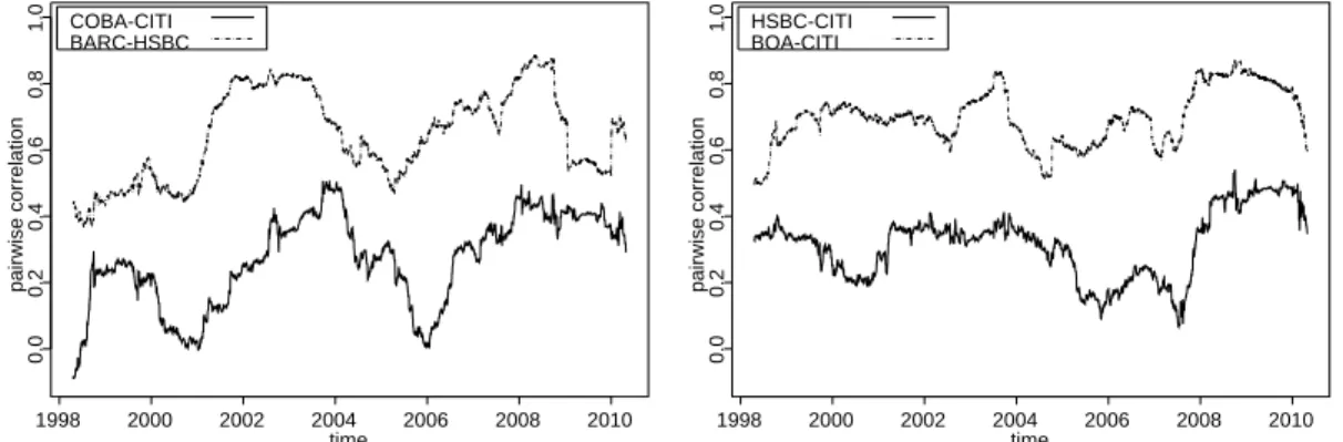
cf. Embrechts et al. (2003). Figure 2.3 shows the estimated evolution of the linear correlation coefficient between the returns of selected pairs of banks. In general, the degree of association between the return series (as e.g. measured by linear correlation) can largely differ. Further, association between financial asset returns is not constant but may change over time.
The linear correlation coefficient is frequently used to measure the amount of associa- tion between two random variables since it is quite tractable from a user perspective and has numerous applications; cf. chapter 1. It represents the natural measure of associa- tion between random variables with a joint normal or elliptical distribution (provided the second moments exist). As already mentioned in the previous chapter, the linear
COBA
BOA
-0.04 -0.02 0.0 0.02 0.04
-0.04-0.020.00.020.04
BOA
CITI
-0.04 -0.02 0.0 0.02 0.04
-0.04-0.020.00.020.04
Figure 2.2: Contour plots of the empirical density of the daily returns of the banks BOA and COBA (left panel) and CITI and BOA (right panel) for the observation period May 1997 to April 2010.
1998 2000 2002 2004 2006 2008 2010
0.00.20.40.60.81.0pairwise correlation
time COBA-CITI
BARC-HSBC
1998 2000 2002 2004 2006 2008 2010
0.00.20.40.60.81.0pairwise correlation
time HSBC-CITI
BOA-CITI
Figure 2.3: Estimated evolution of the linear correlation coefficient between the daily returns of selected pairs of banks for the observation period May 1997 to April 2010, based on a moving window with window size 250.
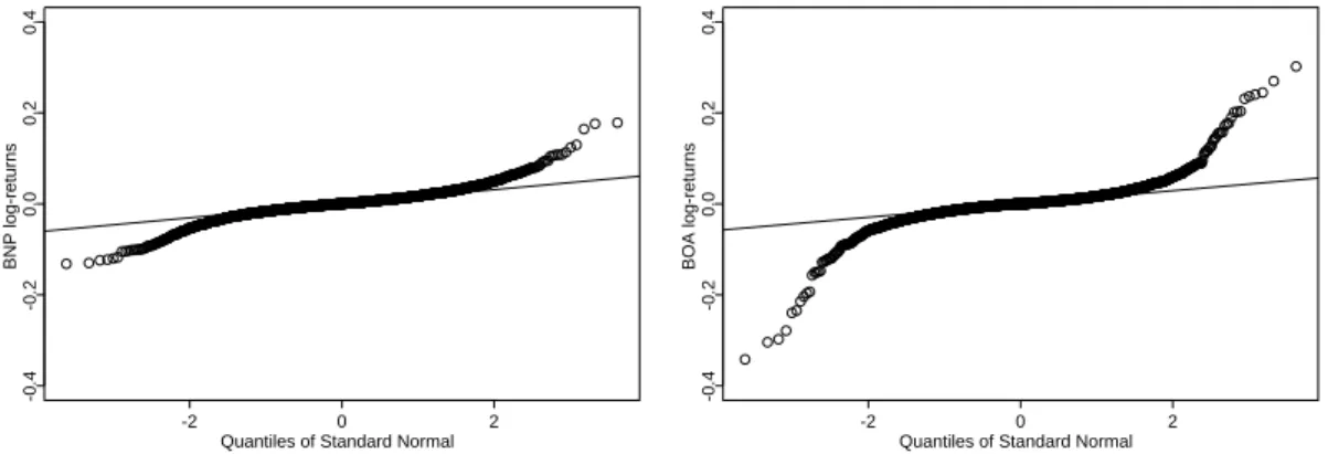
correlation coefficient is a less appropriate measure of association between two random variables if the underlying distribution is non-elliptical. The theory of copulas allows for a more sophisticated modeling of the dependence structure instead. For example, consider the QQ-Plots in figure 2.4 which graphically compare the empirical quantiles of the returns of banks BNP and BOA with the (theoretical) quantiles of a normal distribution. Together with figure 2.2 (left panel), they give strong evidence that the distributions of the two return series are of different tail behavior. In the context of multivariate distribution modeling, note that all marginal distribution functions of a multivariate elliptical distribution have the same shape (except location and scaling).
Copulas allow for the construction of multivariate distribution functions having differ- ent marginal distribution functions.
Quantiles of Standard Normal
BNP log-returns
-2 0 2
-0.4-0.20.00.20.4
Quantiles of Standard Normal
BOA log-returns
-2 0 2
-0.4-0.20.00.20.4
Figure 2.4: QQ-Plots of daily returns of banks BNP and BOA for the observation period May 1997 to April 2010.
As discussed before, measures of association such as Spearman’s rho and Kendall’s tau represent alternatives to the linear correlation coefficient (see section 2.3.3 for their definition). In contrast to the latter, those measures solely depend on the copula of the underlying random variables and are invariant with respect to the marginal distribu- tions. Figure 2.5 provides contour plots of the empirical densities of realizations from two differently distributed bivariate random vectors. Their distributions have differ-
X1
X2
0.0 0.5 1.0 1.5 2.0 2.5
0.00.51.01.52.02.5
Y1
Y2
0.0 0.5 1.0 1.5 2.0 2.5
0.00.51.01.52.02.5
Figure 2.5: Left panel: Contour plot of the empirical density of 10,000 realizations of a random vector (X1, X2) having an equi-correlated Gaussian copula and equally exponentially distributed marginal distributions. Right panel: Contour plot of the empirical density of 10,000 realizations of a random vector (Y1, Y2) having a Clayton copula and equally exponentially distributed marginal distributions.
ent copulas though identical exponentially distributed marginal distribution functions.
Though the plots imply that the association between the components of the random vectors differs, this is not reflected by the value of the linear correlation coefficient, which is almost the same in both samples (see table 2.1). For comparison, we addition- ally give the corresponding values of Spearman’s rho and Kendall’s tau. In contrast
Table 2.1: Estimated values of the linear correlation coefficient, Spearman’s rho, and Kendall’s tau of the realizations of the two random vectors (X1, X2) and (Y1, Y2) as described in figure 2.5.
Linear correlation Spearman’s rho Kendall’s tau
(X1, X2) 0.246 0.293 0.198
(Y1, Y2) 0.243 0.403 0.279
to the linear correlation coefficient, both measures indicate a quantitative difference in the degree of association between the components of the random vectors.
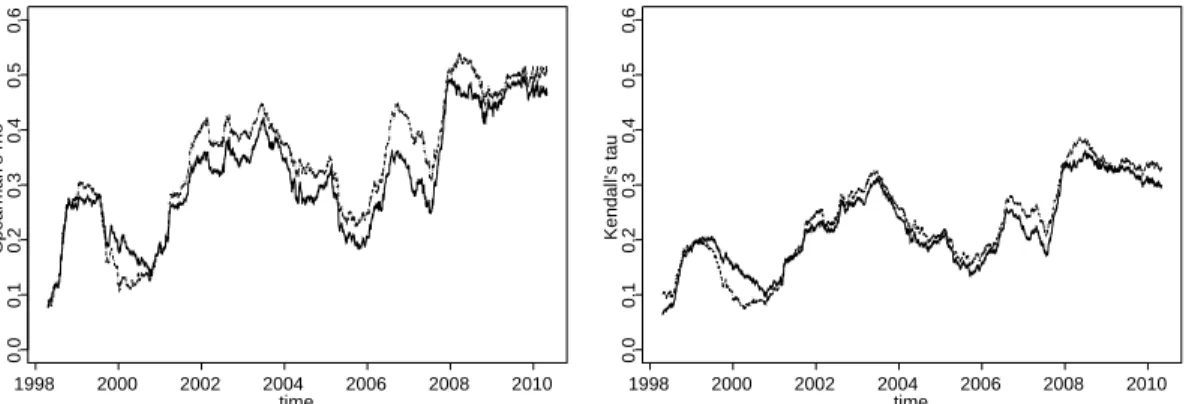
Beside the adequate measurement of association between financial asset returns, it is also of interest to analyze and study diversification effects in a portfolio, especially in portfolio theory. For example, it is important to a portfolio manager how the diversifi- cation in a portfolio changes if one or several assets are replaced. Such diversification effects can be measured using multivariate versions of Spearman’s rho and Kendall’s tau. For illustration, figure 2.6 shows the evolution of Spearman’s rho and Kendall’s tau between the daily returns of two portfolios of five banks each, where the second portfolio results from the first by substituting one bank by another. It becomes appar- ent that the degree of association in the two distinct portfolios differs in several time periods.
1998 2000 2002 2004 2006 2008 2010
0.00.10.20.30.40.50.6Spearman’s rho
time
1998 2000 2002 2004 2006 2008 2010
0.00.10.20.30.40.50.6Kendall’s tau
time
Figure 2.6: Estimated evolution of five-dimensional Spearman’s rho (left panel) and Kendall’s tau (right panel) of the daily returns of banks COBA, BARC, HSBC, BOA, and CITI (solid) and of the daily returns of banks BNP, COBA, BARC, HSBC, and BOA (dotted) for the observation period May 1997 to April 2010.
Measures of association such as Spearman’s rho or Kendall’s tau quantify the de- gree of association between the components of a random vector as determined by its entire distribution function. Another important dependence concept, which we briefly
mention for completeness, is tail dependence. Tail dependence is used in the mod- eling and measurement of association between extreme values such as e.g. extremely negative asset returns and plays a role in financial theory; cf. Joe (1997). In contrast to the mentioned measures of association, measures for tail dependence focus on the tail of the distribution function. For example, the coefficient of upper tail dependence of two random variables X and Y with continuous distribution functions F and G, respectively, is defined as
λU = lim
u→1−IP(Y > G−1(u)|X > F−1(u)),
provided that the limit λU ∈ (0,1] exists. If λU = 0, then X and Y are said to be asymptotically independent in the upper tail. It can be shown that the tail dependence coefficient is a functional of the copula of the underlying random vector.
2.2 Modeling multivariate association - the concept of copulas
Copulas provide a way to analyze the relationship between a multivariate distribu- tion function and its univariate marginal distribution functions. The notion of copulas has been introduced by Sklar (1959) who showed that copulas are functions which bind or join univariate distribution functions to obtain multivariate distribution func- tions. In fact, copulas themselves are multivariate distribution functions with univariate marginal distributions being uniform on the interval [0,1]. The study of copulas is of interest in many fields of research and application. In probability and statistics, copu- las play an important role basically for the following two reasons: They can be used to construct multivariate distribution functions by modeling each univariate marginal dis- tribution function and the copula separately. Further, copulas allow for a sophisticated analysis and modeling of the association between random variables. Especially in the fields of financial and actuarial sciences, copulas have gained in immense importance over the last two decades as they have opened up many new possibilities to consider association between risky assets.
2.2.1 Definition, properties, and examples
We start with the definition of copulas (see Nelsen (2006), p. 10). Note that although the term copula was established by Sklar (1959), many basic results on copulas can be find earlier in the literature, e.g. in the papers by Hoeffding (see Fisher and Sen (1994) for his collected works).
Definition 2.2.1 Let C : [0,1]d → [0,1] be a d-dimensional distribution function on [0,1]d. Then C is called a copula if it has uniformly distributed univariate marginal distribution functions on the interval [0,1].
It immediately follows that all k-dimensional margins of a d-dimensional copula are again copula functions, 2≤k≤d.
The next theorem gives the representation of a multivariate distribution function in terms of its univariate marginal distribution functions and the copula.
Theorem 2.2.2 (Sklar’s theorem) Let F be a d-dimensional distribution function with univariate marginal distribution functions F1, . . . , Fd. Then there exists a d- dimensional copula C such that for all x= (x1, . . . , xd) in Rd,
F(x1, . . . , xd) =C{F1(x1), . . . , Fn(xd)}. (2.2) If F1, . . . , Fd are continuous, then C is unique.
Contrary, if C is a d-dimensional copula and F1, . . . , Fd are univariate distribution functions, then the right-hand side of (2.2) is a d-dimensional distribution function with univariate marginal distribution functions F1, . . . , Fd.
The proof is given in Sklar (1959). It follows from Sklar’s theorem that a multivariate distribution function can be separated into the univariate (continuous) marginal dis- tribution functions and the multivariate dependence structure, which is represented by the copula. Deheuvels (1978) refers to copulas as ’dependence functions’.
For a univariate distribution function G, we define the generalized inverse of G as G−1(u) = inf{x ∈ IR ∪ {∞}|G(x) ≥ u} for all u ∈ (0,1] and G−1(0) = sup{x ∈ IR∪ {−∞}|G(x) = 0}.
Corollary 2.2.3 LetFbe ad-dimensional distribution function with univariate marginal distribution functions F1, . . . , Fd and corresponding copula C satisfying (2.2). Assum- ing that F1, . . . , Fd are continuous, an explicit representation of C is given by
C(u1, . . . , ud) =F{F1−1(u1), . . . , Fd−1(ud)}, u= (u1, . . . , ud)∈[0,1]d. (2.3) This result is a direct consequence from theorem 2.2.2 and is important for the con- struction of copulas from multivariate distributions. If not stated otherwise, we always assume that the univariate marginal distribution functionsF1, . . . , Fd are continuous.
Remarks.
1. According to theorem 2.2.7 in Nelsen (2006), the partial derivatives DiC(u) =
∂C(u)/∂ui of C exist for almost all ui, i = 1, . . . , d. As shown in section 2.2.2, weak convergence of the empirical copula process can be established under mini- mal conditions on those partial derivatives.
2. If ad-dimensional random vector X= (X1, . . . , Xd),defined on some probability space (Ω,F,IP),has distribution functionF with univariate marginal distribution functions F1, . . . , Fd, we also call C as determined by (2.2) the copula ofX.It is denoted by CX orCX1,...,Xd if necessary.
If the marginal distribution functionsF1, . . . , Fdof F are continuous, the transfor- mationXi→ Fi(Xi) is referred to as probability-integral transformation to uniformity
sinceUi =Fi(Xi) ∼U(0,1) in this case , i= 1, . . . d. As implied by (2.2), the copula C (of X having distribution function F) represents the distribution function of the random vector U = (U1, . . . , Ud) and coincides with the copula of the latter random vector. Therefore, many probabilistic investigations concerning copulas can be reduced to the uniform case (see e.g. the proofs of theorems 2.2.8 and 5.2.2 in sections 2.2.2 and 5.2.1, respectively).
We further denote byCthe survival function of the random vectorU= (U1, . . . , Ud) whose distribution function is the copulaC, i.e.,
C(u) = IP(U>u) = IP(U1 > u1, . . . , Ud> ud) for all u∈[0,1]d. (2.4) The survival copula is defined as
C(u) = IP(U˘ >1−u), (2.5)
where 1−u = (1−u1, . . . ,1−ud). The copulaC is said to be radially symmetric if, and only if, it equals its survival copula, i.e.
C(u) = IP(U≤u) = IP(U>1−u) = ˘C(u) for allu∈[0,1]d. (2.6) Every copula is further bounded in the sense that the so called Fr´echet-Hoeffding- bounds inequality holds (see e.g. theorem 2.10.12 in Nelsen (2006)): For ad-dimensional copula C, we have
W(u)≤C(u)≤M(u) for everyu∈[0,1]d, (2.7) with functions M and W, defined on [0,1]d as
M(u1, . . . , ud) = min{u1, . . . , ud}
W(u1, . . . , ud) = max{u1+· · ·+ud−d+ 1,0}.
The upper bound functionM is ad-dimensional copula for all dimensionsd≥2 and is known as the comonotonic copula. If the random vector X has copulaM, each of the random variables X1, . . . , Xd can (almost surely) be represented as strictly increasing function of any of the others. The copula M is also said to describe perfect positive dependence.
In contrast, the lower bound function W is only a copula for dimension d= 2 and is also referred to as the countermonotonic copula in this case. It represents the copula of the bivariate random vector (X1, X2) if there exists a strictly decreasing relationship betweenX1 and X2.Here, the copulaW describes the case of perfect negative depen- dence. According to theorem 2.10.13 in Nelsen (2006), there exists for any d >2 and for anyu∈[0,1]dad-dimensional copulaC⋆such thatC⋆(u) =W(u).The functionW in (2.7) represents thus the ’best-possible’ lower bound and every dependence structure represented by the copula always lies between those two extreme cases. The fact that W fails to be a copula if d > 2 is also closely related to the absence of the concept of perfect negative dependence in this case: For example, if the bivariate random vectors
(X1, X2) and (X2, X3) are perfectly negatively dependent, respectively, then (X1, X3) is perfectly positively dependent and, thus, a three-dimensional perfectly negatively dependent random vector does not exist.
Another important copula is the independence copulaΠ, defined on [0,1]d as Π(u1, . . . , ud) =u1·. . .·ud.
Being a copula for all d ≥ 2, it describes the dependence structure of stochastically independent random variables X1, . . . , Xd.
The behavior of copulas with respect to strictly monotone transformations is es- tablished in the next theorem. Let thereforeβk be a strictly monotone transformation of the kth componentXk of the random vectorX whose domain contains the range of Xk,denoted byRanXk.
Theorem 2.2.4 Let X = (X1, . . . , Xd) be a d-dimensional random vector with dis- tribution function F, continuous marginal distribution functions Fi, i = 1, . . . , d, and copula CX1,...,Xd.
(i) Ifβ1, . . . , βd are strictly increasing on RanX1, . . . , RanXd, respectively, then CX1,...,Xd(u) =Cβ1(X1),...,βd(Xd)(u), u∈[0,1]d.
(ii) Assume thatβ1, . . . , βdare strictly monotone onRanX1, . . . , RanXd, respectively, and let βk be strictly decreasing for some k, without loss of generality let k= 1.
Then, for all u= (u1, . . . , ud)∈[0,1]d,
Cβ1(X1),...,βd(Xd)(u1, . . . , ud) = Cβ2(X2),...,βd(Xd)(u2, . . . , ud)
−CX1,β2(X2),...,βd(Xd)(1−u1, u2, . . . , ud).
For the proof, we refer the reader to Embrechts et al. (2003). Part (i) of the theorem implies that the copula is invariant with respect to strictly increasing transformations of the components ofX.This behavior together with theorem 2.2.2 forms the basis for the role of copulas in the study of multivariate association. According to Schweizer and Wolff (1981), the copula describes precisely those properties of a joint distribution function which do not change under strictly increasing transformations of the margins.
This property is also referred to as ’scale-invariance’ since the study of multivariate association based on copulas is, hence, independent of the scale of the margins. Natu- rally, this is a desirable property of (multivariate) measures of association.
Suppose for the time being that all transformations βi, i = 1, . . . , d, in theorem 2.2.4 are strictly decreasing. Applying part (ii) recursively, we obtain the following relation- ship between the survival copula/survival function and the copula, which we use e.g.
in chapter 4:
Cβ1(X1),...,βd(Xd)(1−u) = X
A⊆Sd
(−1)|A|C(u(A)) = ˘C(1−u) =C(u), (2.8)
where Sd = {1, . . . , d} and, in general, u(A) = (u(A)1 , . . . , u(A)d ) corresponds to the d- dimensional vector u through u(A)j = uj if j ∈ A and u(A)j = 1 otherwise for all sets A ⊆ Sd with cardinality 0 ≤ |A| ≤ d. Note that, if A = {i1, . . . , i|A|}, we also write u(i1,...,i|A|) instead of u(A). The first identity on the left-hand side of formula (2.8) is also studied in Wolff (1980), theorem 2. In particular, it holds that Cβ1(X1),...,βd(Xd) is independent of the particular choice of the transformationsβi, i= 1, . . . , d.For the rep- resentation of ˘CandCin terms of the copula, see also Cherubini et al.(2004), chapter 4.
For more results and background reading on copulas, consult the monographs by Joe (1997) and Nelsen (2006). Regarding their application in finance and risk manage- ment, good references are Embrechts et al. (2003), Cherubini et al. (2004), and McNeil et al. (2005). Let us complete this section by briefly discussing two well-known families of copulas, the elliptical and the Archimedean copulas.
Elliptical Copulas. Elliptical copulas are the copulas of the class of elliptical distributions (see Fang et al. (1990) for a discussion of elliptical distributions) and are constructed according to equation (2.3). In the following, we list two important exam- ples.
Examples. (i) The family of thed-dimensional Gaussian copulas is defined as CG(u1, . . . , ud;K)
=
Z Φ−1(u1)
−∞ · · ·
Z Φ−1(ud)
−∞
(2π)−d2det(K)−12exp
−1
2x′K−1x
dxd. . . dx1, (2.9) with d×d correlation matrix K = (κij)i,j=1,...,d and function Φ denoting the distri- bution function of the univariate standard normal distribution with generalized in- verse function Φ−1.The Gaussian copula CG is called equi-correlated if K =K(κ) = κ1d1′d+ (1−κ)Idwith parameterκsatisfying −1/(d−1)< κ <1.For generalk∈IN, Ik denotes the k-dimensional identity matrix and 1k and 0k correspond to the k- dimensional vectors which solely consist of ones or zeroes, respectively.
(ii) The family of d-dimensional t-copulas is given by
Ct(u1, . . . , ud;K, ν) =tν,K{t−1ν (u1), . . . , t−1ν (ud)}, (2.10) where tν,K denotes the multivariate t-distribution with ν degrees of freedom, location vector zero and correlation matrix K = (κij) (assuming ν > 2) and corresponding univariate marginal distribution functiontν with generalized inverse functiont−1ν .
Random number generation for elliptical copulas is e.g. described in Embrechts et al. (2003), p. 26-27.
Archimedean Copulas. Consider a continuous and strictly decreasing function φ: [0,1]→[0,∞] such that φ(1) = 0.The function C given by
C(u, v) =φ[−1]{φ(u) +φ(v)} (2.11)
is a bivariate Archimedean copula if and only ifφis convex; cf. Nelsen (2006), chapter 4. Here, the function φ[−1] denotes the pseudo-inverse of φ, defined by
φ[−1](t) =
φ−1(t) f or 0≤t≤φ(0) 0 f or φ(0)≤t≤ ∞
The function φis called the generator of the copulaC. Ifφ(0) =∞,the generatorφis is said to be strict andφ[−1]=φ−1.
The approach in formula (2.11) can naturally be extended to d(d≥2) dimensions by imposing additional assumptions onφ.With continuous, strictly decreasing functionφ such that φ(1) = 0 and φ(0) =∞,a d-dimensional Archimedean copula is given by
C(u1, . . . , ud) =φ−1{φ(u1) +· · ·+φ(ud)}
if and only if the inverseφ−1is completely monotone on [0,∞),i.e., if it has derivatives of all orders which alternate in sign; formally, (−1)k ddtkkφ−1(t)≥0 for all t≥0 and all k∈IN.
Examples. (i) Let φ(t) = (−lnt)θ, θ ≥ 1, which generates the d-dimensional Gumbel family
CGu(u1, . . . , ud;θ) = exp [−{(−lnu1)θ+· · ·+ (−lnud)θ}1/θ]. (2.12) (ii) With φ(t) = (t−θ)/θ, θ >0,we obtain thed-dimensional Clayton family
CCl(u1, . . . , ud;θ) = (u−θ1 +· · ·+u−θd −d+ 1)−1/θ. (2.13) A statistical hypothesis test based on the copula-based measure of association Spearman’s rho (cf. section 2.3.3) which can be used to verify whether the choice of an Archimedean copula is appropriate in multivariate distribution modeling is discussed in chapter 5. In general, there exist several methods to generate random numbers from a given Archimedean copula; if needed, we use the method proposed by Marshall and Olkin (1988). For the discussion of the general class of hierarchical Archimedean cop- ulas and related random number generation, we refer to Savu and Trede (2008) and Hofert (2008).
2.2.2 Statistical inference: The empirical copula (process)
Depending on the assumptions made on the joint and the univariate marginal distri- bution functions, we distinguish three general methods for the estimation of copula functions: parametric, semiparametric and nonparametric methods. The parametric and semi-parametric estimation approaches are usually based on maximum-likelihood
methods, we mention Genest and Rivest (1993), Genest et al.(1995), Joe and Xu (1996), Joe (2005), Chen and Fan (2006), and Kim et al.(2007). For an overview see also Malev- ergne and Sornette (2005), chapter 5. In this thesis, we solely consider nonparametric estimation methods for which the joint and the marginal distribution functions are assumed to be unknown. In particular, this method is not exposed to possible misspec- ifications of the underlying distributions, see Charpentier et al. (2007) for related pit- falls. Nonparametric estimation of copulas was first considered by R¨uschendorf (1976) and Deheuvels (1979) who proposed the so called empirical copula as a nonparametric estimator.
Nonparametric estimation
Consider thed-dimensional random vectorXwith distribution functionF,continuous univariate marginal distribution functionsFi, i= 1, . . . , d, and copula C. Assume that F, C,andFi are completely unknown and letX1, . . . ,Xn be a random sample fromX.
The empirical copula is built in two steps. First, every univariate marginal distribution functionFi is estimated by its univariate empirical distribution function, i.e.,
Fbi,n(x) = 1 n
Xn j=1
1{Xij≤x} fori= 1, . . . , dand x∈R.
The estimated marginal distribution functions are then used to obtain the so called pseudo-observationsUbij,n =Fbi,n(Xij) with Ubj,n = (Ub1j,n, ...,Ubdj,n) for i= 1, ..., d, j = 1, ..., n.Finally, an estimate of the copula Cis given by the empirical distribution func- tion of the sampleUb1,n, . . . ,Ubn,n.The latter is typically called the empirical copula and was introduced by Deheuvels (1979) under the name ’empirical dependence function’.
Definition 2.2.5 Let X be a d-dimensional random vector with distribution function F,continuous univariate marginal distribution functionsFi, i= 1, . . . , d, and copulaC.
Based on a random sample X1, . . . ,Xn from X, the empirical copula is defined as Cbn(u) = 1
n Xn j=1
Yd i=1
1{Ub
ij,n≤ui}, for u∈[0,1]d, (2.14) withUbij,n as introduced above.
Since Ubij,n = 1/n(rank ofXij inXi1, ..., Xin),the empirical copula represents a rank- based estimator for the copulaC, i.e., only the (normalized) ranks of the observations are included in the estimation. According to definition 2.2.1, the empirical copula itself is a copula. In particular, it is invariant under strictly increasing transformations of the margins (cf. theorem 2.2.4, part (i)) due to the invariance property of the ranks with respect to such transformations. According to Genest and Favre (2007), the ranks as- sociated with the random sampleX1, . . . ,Xn are the statistics that retain the greatest amount of information among all statistics fulfilling this invariance property. For fixed