Structure and distribution of a threatened muddy biotope in the south-eastern
1
North Sea
2
3
Lars Gutow1*, Carmen-Pia Günther2, Brigitte Ebbe1, Sabine Schückel2, Bastian Schuchardt2, 4
Jennifer Dannheim1,3, Alexander Darr4, Roland Pesch2,5 5
6
1Alfred Wegener Institute Helmholtz Centre for Polar and Marine Research, Am Handelshafen 7
12, 27570 Bremerhaven, Germany 8
2BioConsult Schuchardt & Scholle GbR, Auf der Muggenburg 30, 28217 Bremen, Germany 9
3Helmholtz Institute for Functional Marine Biodiversity, Ammerländer Heerstraße 231, 26129 10
Oldenburg, Germany 11
4Leibniz Institute for Baltic Sea Research, Seestraße 15, 18119 Rostock-Warnemünde, 12
Germany 13
5Institute for Applied Photogrammetry and Geoinformatics (IAPG), University of Applied 14
Sciences, Oldenburg 15
16
*Corresponding author: email: lars.gutow@awi.de; phone: +49 471 4831 1708 17
18
Abstract 19
Understanding the distribution and structure of biotopes is essential for marine conservation 20
according to international legislation, such as the European Marine Strategy Framework 21
Directive (MSFD). The biotope ‘Sea Pen and Burrowing Megafuna Communities’ is included in 22
the OSPAR list of threatened and/or declining habitats. Accordingly, the MSFD prescribes a 23
monitoring of this biotope by the member states of the EU. In the German North Sea, 24
however, the distribution and spatial extent of this biotope as well as the structuring of its 25
benthic species inventory is unknown. We used an extensive geo-referenced dataset on 26
occurrence, abundance and biomass of the benthic infauna of the south-eastern North Sea to 27
estimate the distribution of the biotope and to characterize the associated infauna 28
assemblages. Sediment preferences of the burrowing megafauna, comprising decapod 29
crustaceans and echiurids, were identified and the core distribution areas of the burrowing 30
megafauna were modelled using Random Forests. Clusters of benthic infauna inside the core 31
distribution areas were identified by fuzzy clustering. The burrowing megafauna occurred on 32
a wide range of sediments with varying mud contents. The core distribution area of the 33
burrowing megafauna was characterized by elevated mud content and a water depth of 25- 34
55 m. The analysis of the benthic communities and their relation to sedimentological 35
conditions identified four infauna clusters of slightly varying species composition. The biotope 36
type ‘Sea Pen and Burrowing Megafuna Communities’ is primarily located inside the paleo 37
valley of the river Elbe and covers an area of 4980 km2. Dedicated monitoring will have to take 38
into account the spatial extent and the structural variability of the biotope. Our results can 39
provide a baseline for the evaluation of the future development of the environmental status 40
of the biotope. The maps generated herein will facilitate the communication of information 41
relevant for environmental management to authorities and policy makers.
42 43
Keywords: Marine benthos, marine conservation, German Bight, spatial modelling, sediment 44
preference 45
46
Introduction 47
The biotope is a basic concept in marine benthic conservation and spatial planning. In this 48
context, a benthic biotope is defined by its distinct physico-chemical and geo-morphological 49
seafloor environment (i.e. the habitat) and the specific assemblage of species inhabiting this 50
particular environment (Olenin and Ducrotoy 2006). The composition of benthic species 51
assemblages is strongly shaped by the environmental conditions, with sediment 52
characteristics and water depth being, among others, important determinants of species’
53
occurrence (Gray 1974, Reiss et al. 2011, Armonies et al. 2014). The vast geomorphological 54
heterogeneity of the seafloor at various spatial scales and the high diversity of the benthic 55
biota has led to the classification of numerous different seafloor biotopes in European waters 56
and beyond (Davies et al. 2004). According to international legislative frameworks to protect 57
the marine environment, such as the European Marine Strategy Framework Directive (MSFD, 58
2008/56/EC), member states of the European Union are obliged to carry out an assessment 59
and continuous monitoring of widespread and specific benthic biotopes. The results from the 60
mandatory monitoring programs provide the basis for an evaluation of the environmental 61
status of the marine environment and the effectiveness of management and conservation 62
measures.
63
The development and implementation of successful biotope monitoring programs requires 64
knowledge of the distribution, the spatial extent and the structure of biotopes in order to 65
determine the appropriate temporal and spatial resolution of sampling activities (Van der 66
Meer 1997). Often, however, information on the exact geo-morphological characteristics, the 67
faunal composition, and the spatial distribution of specific biotopes is limited. Additionally, 68
functional aspects are being increasingly considered in the definition of biotopes accounting 69
for the importance of crucial ecological processes for achieving and maintaining a good 70
environmental status of sensitive marine ecosystems (Berg et al. 2015). Decades of research 71
have generated extensive, highly resolved datasets on the distribution of benthic species and 72
environmental variables in many shelf sea areas. Along with an advanced understanding of 73
the factors that shape benthic communities (Pesch et al. 2008) these datasets suggest a 74
complex structuring of benthic biotopes, which are on a regional scale often linked with broad 75
sediment features, such as mud content (Degraer et al. 2008).
76
Continuous discharge of large quantities of suspended organic matter and finest sediment 77
fractions by major rivers have formed extensive areas of muddy sediments in the German 78
Bight (south-eastern North Sea), especially off the mouth of the river Elbe and along its paleo 79
river valley extending towards the central North Sea. The organic content of muddy sediments 80
sustains a considerable species richness and biomass of the benthic fauna (Duineveld et al.
81
1991), which itself provides a valuable food resource for organisms at higher trophic levels of 82
the marine food web, such as (commercially important) fish (Greenstreet et al. 1997).
83
Moreover, muddy biotopes are sensitive to environmental and physical stressors such as 84
oxygen limitation, pollution, and bottom trawling (Rachor 1977, Kaiser et al. 2006).
85
An ecologically important functional attribute of mud is the cohesiveness of the sediment 86
that allows certain infaunal organisms to construct and sustain persistent burrows. The 87
penetration depth for oxygen in fine-grained muddy sediment is low (Brotas et al. 1990) and 88
high microbial activity may lead to oxygen depletion and formation of toxic hydrogen sulfide 89
(Rachor 1977). Burrowing organisms, including some decapod crustaceans and echiurids, 90
enhance the ventilation of the sediment by flushing their burrows, a process referred to as 91
bio-irrigation (Meysman et al. 2006). By providing oxygen and nutrients to micro-organisms in 92
deeper sediment layers burrowing organisms support important sediment-bound bio- 93
geochemical processes, the recycling of nutrients from organic matter and, thus, marine 94
primary and secondary production (Lohrer et al. 2004). To account for these important 95
ecological functions and for the sensitivity of benthic organisms to, for example, mechanical 96
damage induced by continuous bottom trawling, the biotope type ‘Sea pen and burrowing 97
megafauna communities’ was included in the OSPAR list of threatened and/or declining 98
habitats (OSPAR 2008a). The biotope is defined as “Plains of fine mud, at water depths ranging 99
from 15-200 m or more, which are heavily bioturbated by burrowing megafauna with burrows 100
and mounds typically forming a prominent feature of the sediment surface. The habitat may 101
include conspicuous populations of seapens, typically Virgularia mirabilis and Pennatula 102
phosphorea. The burrowing crustaceans present may include Nephrops norvegicus, Calocaris 103
macandreae or Callianassa subterranea. In the deeper fjordic lochs, which are protected by 104
an entrance sill, the tall seapen Funiculina quadrangularis may also be present. The burrowing 105
activity of megafauna creates a complex habitat, providing deep oxygen penetration. This 106
habitat occurs extensively in sheltered basins of fjords, sea lochs, voes and in deeper offshore 107
waters such as the North Sea and Irish Sea basins” (OSPAR 2008b). Sea pens are entirely 108
lacking in the south-eastern North Sea. However, according to the above definition the 109
occurrence of sea pens is not mandatory for this biotope to be present.
110
As a threatened or declining habitat according to OSPAR, the biotope ‘Sea pen and 111
burrowing megafauna communities’ has to be considered as a specific biotope according to 112
the MSFD in the mandatory environmental monitoring programs of member states of the EU.
113
Besides this muddy biotope, a single additional MSFD specific biotope (‘Species-rich coarse 114
sand and shell gravel bottoms’ – protected under the German Federal Law of Nature 115
Conservation) exists in offshore regions of the German North Sea. The remaining extensive 116
seafloor areas in this region constitute the MSFD broad biotope ‘Offshore sands’. Detailed 117
characterizations of the biotopes, including sedimentological and ecological characteristics, as 118
well as information on their spatial extent and distribution in the German North Sea are still 119
lacking. Furthermore, only little is known about the structural variations of the benthic faunal 120
assemblages associated with the biotopes. However, this information is essential for 121
successful marine environmental management and conservation according to the MSFD, 122
which aims at achieving a good environmental status of European marine waters. Defining the 123
good environmental status and evaluating the actual status requires a proper monitoring 124
based on sound knowledge on the distribution and structure of biotopes and the inherent 125
spatial and temporal variability. Additionally, this knowledge is needed for marine spatial 126
planning, for example, for the designation of marine protected areas (Degraer et al. 2008).
127
This study on a protected seafloor biotope generates important information for 128
management and conservation from an extensive geo-referenced data set on the benthic 129
macro-infauna of the German North Sea. Specifically, we describe the distribution and 130
sedimentological preferences of organisms belonging to the burrowing benthic megafauna, 131
including thalassinidean crustaceans (‘mud shrimps’) and echiurids. The full coverage 132
distribution of the muddy biotope is modelled based on the occurrence of the burrowing 133
benthic megafauna in combination with sedimentological and topographical geodata. Finally, 134
the benthic infauna assemblages associated with the biotope are described in terms of 135
characteristic species to achieve a comprehensive sedimentological, bathymetric and 136
biological characterization of the OSPAR biotope type of the German North Sea. Maps are 137
provided, which will facilitate the planning of an appropriate monitoring of the protected 138
biotope in the German North Sea to support management and conservation according to 139
international legislative frameworks.
140 141
Material and methods 142
Study area 143
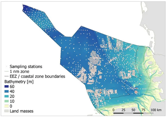
This study addresses the German Exclusive Economic Zone (EEZ) and the German coastal 144
waters >1 nm off the coast in the south-eastern North Sea (Figure 1). The area covers about 145
35,000 km2 and stretches from the North and East Frisian coasts towards the easternmost 146
offset of the Dogger Bank, which separates the coastal waters of the south-eastern coastal 147
North Sea from the waters of the more oceanic central North Sea. The sediment types cover 148
the full range from extensive areas dominated by muddy and sandy sediments to more patchy 149
stretches of coarse sand and scattered glacial depositions of rocks and boulders, which are 150
primarily found around the rocky island of Helgoland, the Sylt Outer Reef, Borkum Reef 151
Ground and off the island of Sylt (Diesing et al. 2006, Michaelis et al. 2019). A dominant 152
geomorphological structure of the southern North Sea is the paleo valley of the river Elbe, 153
which extends from the present day Elbe river mouth in north-western direction towards the 154
central North Sea. The seafloor of the paleo river valley is characterized by sediments with 155
elevated mud content and it traverses extensive areas of fine sandy sediments (Figge 1981).
156
The discharge of the river Elbe enhances the organic load of the muddy sediment inside the 157
river valley.
158 159
160
Figure 1: Bathymetry of the south-eastern North Sea with sampling stations for benthic 161
infauna 162
163
Major associations of benthic infauna species broadly match the distribution of the 164
dominant sediment types in the south-eastern North Sea (Salzwedel et al. 1985, Reiss et al.
165
2010, Neumann et al. 2013). The south-eastern North Sea is a shallow marine region with 166
water depths off the intertidal Wadden Sea ranging from 20 to 60 m (Bockelmann et al. 2018).
167
The benthic system of the region is strongly influenced by exceptional meteorological events, 168
such as extremely low winter temperatures (Reiss et al. 2006). Moreover, bottom-near 169
hypoxia can develop during seasonal stratification of the water body, especially in summer.
170
The average sea surface temperature in the southern North Sea ranges from 3°C in winter to 171
18°C in summer (Elliot et al. 1991). The salinity varies between 30 PSU in coastal waters and 172
35 PSU in offshore waters (Skov and Prins 2001). Dominant hydrographic and oceanographic 173
features, including persistent frontal systems and gyres, shape the distribution and residence 174
time of water masses and the dissolved and suspended matter therein (Dippner 1993).
175
176
Data origin 177
The analyses performed in this study are based on an extensive dataset on the benthic 178
infauna of the German North Sea. Over the years 1997 to 2016 data were collected from 8883 179
infauna stations within various ecological long-term programs, research projects, and impact 180
assessments studies for approval procedures for industrial offshore projects, including wind 181
farm constructions and underwater cables. For 64 % of the stations the data on the infauna 182
were generated from a single van Veen grab (area: 0.1 m2, weight: 90 kg) whereas three grab 183
samples per station were taken at 36 % of the stations. The samples were sieved (mesh size:
184
1000 µm), and stored in buffered 4 % formalin-seawater solution for further processing in the 185
laboratory. In the laboratory, the samples were washed with freshwater. All organisms of the 186
benthic macro-infauna were extracted and determined to the lowest taxonomic level possible.
187
All individuals were counted and the biomass (wet weight) was determined at the species 188
level. Colonial organisms were not counted but recorded as present. Sedimentological 189
information was available for 4549 stations sampled between the years 2000-2016. Sub- 190
samples for the sediment analysis were taken either from a fourth grab or from one of the 191
infauna grabs. Each sub-sample was dried and sieved through a sieve cascade (Wentworth 192
1922). The fraction that passed through the sieve with a mesh size of 63 µm was weighed to 193
determine the mud content (%).
194 195
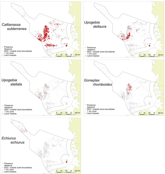
Borrowing megafauna occurrence and sediment composition 196
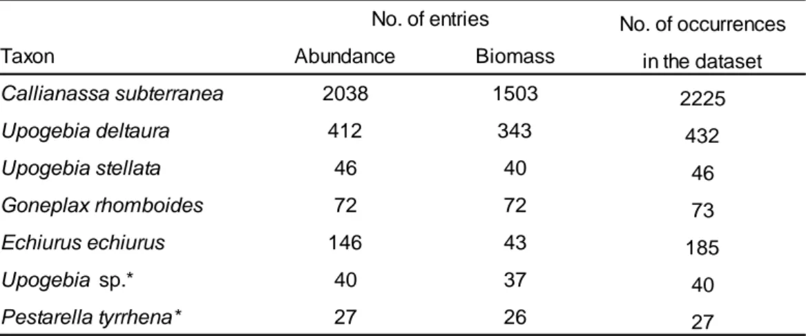
Five species of the burrowing megafauna were considered for the analysis: Callianassa 197
subterranea, Goneplax rhomboides, Echiurus echiurus, Upogebia deltaura and Upogebia 198
stellata (for data availability and selection of species for analysis see the supplementary 199
material as well as Figure S1 and Table S1). The relationship between sedimentological 200
characteristics and the occurrence of species of the burrowing megafauna was analysed from 201
abundance and biomass data (averaged by station) at those stations, for which information 202
was available on both abundance and/or biomass of the species and the mud content of the 203
sediment. For 2200 stations abundance data were available for at least one megafauna 204
species. For 1600 of these stations additional data on biomass were available. For each taxon, 205
abundance and biomass were tested for correlation with the mud content of the sediment 206
using correlation analysis. To account for non-normality in the data distributions and missing 207
linear relationships between abundance/biomass and mud content, coefficients of correlation 208
were calculated according to Spearman (1904).
209
All stations were assigned to one of six classes according to the mud content of the 210
sediment: <5 %, 5-10 %, >10-20 %, >20-50 %, >50-80 %, and >80 %. Each taxon was tested for 211
differences in abundance and biomass between the classes using non parametric pairwise 212
tests according to Wilcoxon as available in the R package ‘coin’ (Hothorn et al. 2008). Test 213
statistics were calculated from permutations of the input data by Monte Carlo approximations 214
based on 10,000 permutations drawn from the original data set. Variations in taxon specific 215
abundances and biomasses among sediments with different mud contents are displayed in 216
Box-Whiskers-graphs with statistically significant differences being indicated by different 217
letters.
218 219
Core areas of distribution of the burrowing megafauna in the German North Sea 220
Core areas of the distribution of the burrowing megafauna in the German North Sea (i.e., 221
German EEZ plus coastal waters of ≥1 nm distance from the shore) were identified using 222
Random Forests (Breimann 2001). Random Forests is a machine learning method to derive 223
prediction models for target variables of either metric, ordinal or nominal levels of 224
measurement from chosen predictor variables. Due to its robustness Random Forests has 225
successfully been applied in previous studies to predict both biotic and abiotic characteristics 226
of the seafloor (Darr et al. 2014, Diesing et al. 2014, Gonzalez-Mirelis et al. 2011, Lindegarth 227
et al. 2014, Šiaulys and Bučas 2012). Derived from Classification and Regression Trees (CART 228
– Breimann et al. 1984) Random Forests calculates a multitude of independent decision trees 229
from bootstrap samples of the original data. The decision trees can then be used to predict 230
the variable of interest for objects (here: grid cells), where information on the predictor 231
variables is available. If the target variable is categorical, the category is assigned to a given 232
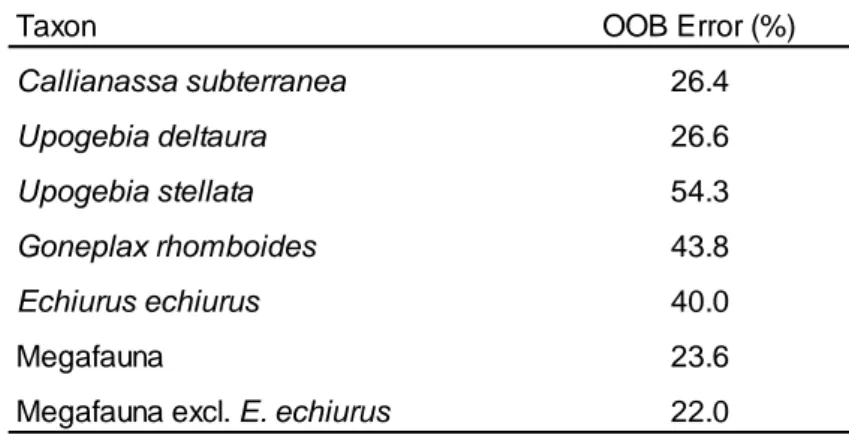
object that was predicted from most of the independent decision trees. Globally, the quality 233
of Random Forests models can be described by the Out of Bag (OOB) Error, which is calculated 234
by the above mentioned independent decision trees produced within Random Forests. As all 235
decision trees rely on randomly chosen bootstrap samples from the total data set they can 236
each be applied to the remaining data to quantify whether true or observed categories were 237
classified correctly. Correspondingly, the OOB Error is the average error rate over all 238
categories and observations and is given as percentage. A further global reliability measure of 239
classification is the Kappa coefficient of agreement according to Cohen (1960), which can be 240
calculated from the confusion matrix provided by Random Forests. Cohen’s Kappa 241
corresponds to the proportion of agreement corrected for chance and takes values between 242
0 (highest possible classification disagreement) and 1 (highest possible classification 243
agreement).
244
In total, data from all 8883 stations from the years 1997-2016 were used for the modelling 245
of core distribution areas via Random Forests. The occurrence (presence/absence) of the 246
megafauna taxa were used as target variables because high spatial and temporal variability of 247
abundance and biomass led to constantly low degrees of explained variance in corresponding 248
random forest models (each r2 < 0.3). As predictors we used the UTM 32-coordinates 249
(according to recommendations given by Evans et al. 2011), full coverage data on bathymetry 250
(Populus et al. 2017), geo-statistically interpolated sand, gravel and mud fractions (Schönrock 251
2016) as well as an ordinal mud index derived from the map on sediment types for the German 252
North Sea according to the classification by Figge (1981). The map was available at a spatial 253
resolution of 1:250,000 (Laurer et al. 2013) and provided information on 22 sediment types 254
including coarse sands, medium coarse sands, medium sands, fine sands, and mud for most 255
parts of the German North Sea. For some areas in the outer German EEZ (i.e. 2.1 % of the 256
entire study area) no information on sediment types were given in the map due to missing 257
primary data on grain sizes (Laurer et al. 2013). These areas could, thus, not be considered in 258
the Random Forests modelling. The percentages mud content were assigned for each sand 259
fraction to one of the following classes: <5 %, 5-10 %, >10-20 %, >20-50 %, >50-80 %, and >80 260
%. These classes were used to derive the ordinal mud index ranging from 1 (<5 % mud) to 6 261
(>80 % mud). All presence/absence data for the megafauna taxa were intersected with the 262
full coverage maps, which were harmonized to a 230 x 230 m grid according to the resolution 263
provided by the map on the geostatistical grain size maps by Schönrock (2016). The application 264
of the grid led to the aggregation of records within single cells, which may have affected the 265
model performance (in terms of OOB Error and Kappa). However, given the great spatial 266
coverage of the data set we expect no effects on the modelled core distribution areas of the 267
burrowing megafauna. All geo-processing tasks were performed using the software packages 268
QGIS 2.18 and ArcGIS 10.4.
269
Random forests modelling was done based on 5000 classification trees for each taxon, and 270
three out of the seven predictors were chosen for the bootstrap samples. The random forests 271
modelling was performed in R version 3.4.0. using the package ‘random forests’ (Liaw and 272
Wiener 2002). The adequate presence threshold for each taxon was determined using the R 273
package ‘Presence Absence’ (Freeman and Moisen 2008). Thresholds were derived using the 274
method ‘Sens=Spec’ so that modelled positive observations are equally likely to be wrong as 275
negative observations.
276
Random Forests models were calculated individually for each taxon of the burrowing 277
megafauna. However, for most of the taxa the OOB Errors were high, especially for E. echiurus, 278
G. rhomboides and U. stellata (Table S2). Therefore, an additional model was calculated using 279
the combined occurrence data of all taxa of the burrowing megafauna resulting in an 280
acceptable rate of misclassification of <25 %. An additional model was calculated excluding 281
the species E. echiurus, which showed a distribution that was largely disconnected from the 282
other species, resulting in a further improvement of the rate of misclassification to 22 %.
283
Therefore, the core distribution areas of the burrowing megafauna presented in this study, 284
were subsequently based on the model, which was calculated excluding E. echiurus. The 285
modelled core distribution areas were described by the above described full coverage 286
information on bathymetry and the station-specific mud content (%) and contrasted with the 287
remaining areas of the German North Sea.
288 289
Infauna communities inside the core areas 290
Specific infauna communities were identified from a total of 4251 stations sampled inside 291
the core distribution areas of the burrowing megafauna during the years 1997-2016 using the 292
fuzzy k means clustering approach (Bezdek 1981) as available in the R package fclust (Ferraro 293
and Giordani 2015). Different from commonly used hierarchical cluster approaches in benthic 294
ecology, fuzzy k means clustering is an iterative, partitioning clustering algorithm to achieve 295
optimal cluster homogeneity accounting for non-crisp assignments of objects (here: stations 296
attributed by taxon abundances) to the resulting clusters. The uncertainty of assigning a given 297
cluster to a chosen monitoring station is quantified in terms of a fuzzy membership ranging 298
from 0 (i.e. minimum strength of affiliation to a given cluster) to 1 (i.e. maximum strength of 299
affiliation to a given cluster). A fuzzy clustering approach was preferred over other crisp 300
clustering techniques, such as hierarchical clustering, because previous applications in biotope 301
mapping identified plausible infauna communities in the German North Sea (Fiorentino et al.
302
2017; Pesch et al. 2015). Furthermore, fuzzy clustering results allow for alternative mapping 303
procedures for selected biotopes of interest (Schönrock et al. in press) and calculating the 304
Fuzzy Silhouette index as an alternative clustering validity measure (Ferraro and Giordani 305
2015). The Fuzzy Silhoutte criterion performs equally well or even better than other cluster 306
validity criteria (Campello and Hruschka 2006). Therefore, the Fuzzy Silhouette index was 307
selected to evaluate different numbers of benthic infauna clusters (Ferraro and Giordani 308
2015).
309
The fuzzy k means clustering algorithm was applied to Hellinger transformed abundance 310
data from all stations sampled inside the core areas (Rao 1995, Legendre and Legendre 1998, 311
Legendre and Gallagher 2001, Borcard et al. 2011). Solutions with two, three, four and five 312
clusters, respectively, were calculated and the highest quality of the cluster solution was 313
identified at maximum values of the Fuzzy Silhouette index (Campello and Hruschka 2006).
314
For each cluster solution, characteristic species of the infauna community were identified 315
according to Salzwedel et al. (1985) modified after Rachor and Nehmer (2003) and Rachor et 316
al. (2007). A species was accepted as characteristic for an assemblage if at least three out of 317
the following five criteria were met:
318
(1) Numerical dominance – ND: numerical dominance within the assemblage (abundance 319
of a species divided by the total abundance of the assemblage) 320
(2) Presence – P: presence within the association (proportion of stations within the 321
assemblage the species was found at) 322
(3) Fidelity in abundance – FA: degree of association regarding individuals (number of 323
individuals of a species in the assemblage divided by the number of individuals of that 324
species in the entire study area) 325
(4) Fidelity in presence – FP: degree of association regarding stations (number of stations 326
within an assemblage the species was found at divided by number of stations that 327
species was found at in the entire study area) 328
(5) Rank of dissimilarity – RD: rank of species contribution to dissimilarity of a cluster group 329
compared with all other stations determined by SIMPER analysis (Clarke and Warwick 330
1994) 331
Threshold values were set to ND > 3 %, P > 60 %, FA > 50 %, FP > 50 % and RD according to 332
ranks 1 to 8. These threshold values were less strict than those applied by Rachor et al. (2007), 333
which did not allow to identify characteristic species for each cluster because of the high 334
structural similarities among the clusters in the muddy sediments.
335
The definition of the OSPAR biotope ‘Sea pen and burrowing megafauna communities’
336
specifically refers to muddy habitats as the cohesiveness of muddy sediments allows for the 337
construction and maintenance of complex infaunal burrow structures. The cohesiveness of 338
sediment is fundamentally dependent on the clay content. At a clay content of about 10 %, 339
the erosion behaviour of sediment shifts from non-cohesive to cohesive (van Ledden et al.
340
2004). In our data set, the mud fraction of the sediment was characterized by a grain size <63 341
µm without distinguishing between silt and clay. Therefore, we defined sediments as being 342
muddy at a mud content >10 %. The average (± SD) mud content of the sediment was 343
calculated for each cluster and tested for deviation from 10 % using the perm Test routine of 344
the R package jmuOutlier (Higgins 2004, Garren 2017). All cluster solutions were spatially 345
extrapolated for the core distribution areas of the burrowing megafauna by Random Forests 346
using the above listed predictor variables. For each of the two, three, four and five cluster 347
solutions cluster categories were used as target variables by assigning the cluster to each 348
station that showed the highest fuzzy membership score.
349 350
Results 351
Burrowing megafauna occurrence and sediment composition 352
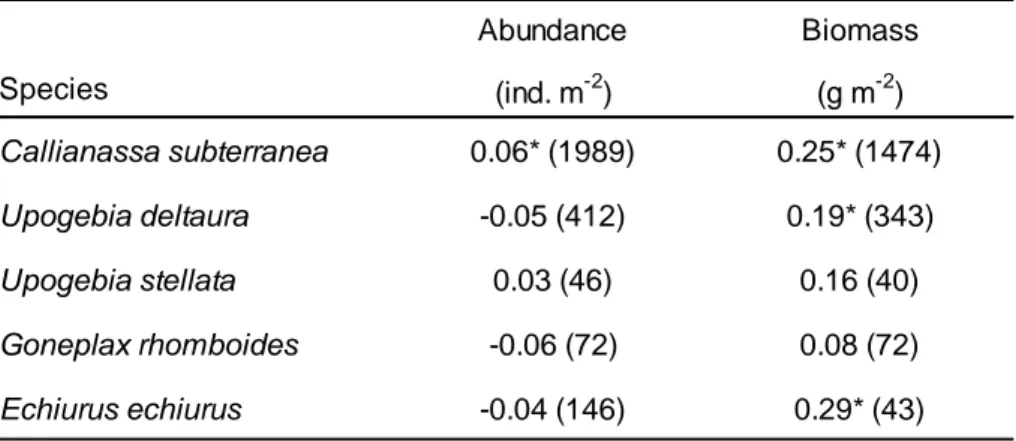
Abundance and biomass of Callianassa subterranea were both positively correlated with 353
the mud content (grain size faction <63 µm) of the sediment (Table 1). The correlation 354
coefficients were low but the relationships were statistically significant. The abundance of 355
Upogebia deltaura was not related to the mud content of the sediment whereas the biomass 356
of this species increased significantly with the mud content. For Upogebia stellata and 357
Goneplax rhomboides no relationships could be confirmed between abundance and biomass, 358
respectively, and the mud content of the sediment. The strongest positive correlation with 359
the mud content was identified for the biomass of Echiurus echiurus whereas the abundance 360
of this species was not related to the mud content.
361 362
Table 1: Results of Spearman correlation analysis to test for correlations between abundance 363
and biomass of taxa of the burrowing megafauna and the mud contents of sediments in the 364
German North Sea. The numbers give the correlation coefficients (r). Numbers in parentheses 365
give the number of replicates. Due to zero inflation absence data were excluded from the 366
analysis. Significant correlations are marked with asterisks.
367
368 369
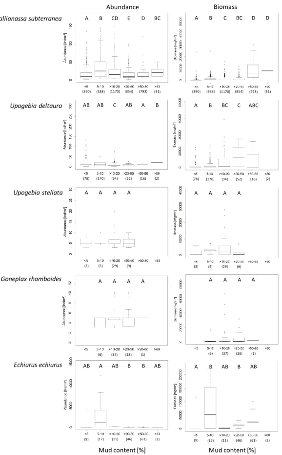
Abundance of C. subterranea was highest in sediments with a mud content of >5-10 % 370
(Figure 2). The abundance was significantly higher in this sediment than in any other sediment 371
except for sediment with the highest mud content above 80 %. The biomass of C. subterranea 372
was highest in sediments with high mud contents (>50 %).
373
The abundance of U. deltaura varied only little with the mud content of the sediment but 374
was significantly reduced in sediment with a mud content of >10-20 %. The biomass of U.
375
deltaura increased towards sediments with increasing mud content (>10 %) but only very few 376
records for this species were available from sediments with the highest mud content (>80 %).
377
Abundances and biomass of U. stellata and G. rhomboides did not show any relationship 378
with the mud content of the sediment. However, both species were entirely missing from 379
sediments with highest mud contents.
380
The abundance of E. echiurus was highest in sediment with a mud content of >5-10 % but 381
low on all other sediment types. The variations were mostly not significant. There were only 382
very few records of E. echiurus and no biomass record from sediments with a mud content 383
>80 %. The median biomass of E. echiurus was highest in sediments with a mud content of >5- 384
10 % but also increased towards sediments with elevated mud content (>20 %).
385
Abundance Biomass
Species (ind. m-2) (g m-2)
Callianassa subterranea 0.06* (1989) 0.25* (1474)
Upogebia deltaura -0.05 (412) 0.19* (343)
Upogebia stellata 0.03 (46) 0.16 (40)
Goneplax rhomboides -0.06 (72) 0.08 (72)
Echiurus echiurus -0.04 (146) 0.29* (43)
386
Figure 2: Abundance (ind. m-2 – left-hand panel) and biomass (g m-2 – right-hand panel) 387
distributions of species of the burrowing megafauna in sediments with different mud contents 388
(%) in the German North Sea. Letters display the results of permutation tests: boxes that share 389
the same letter are statistically not different. Number in brackets give the number of 390
occurrences of the respective species in the dataset.
391
Abundance Biomass
Callianassa subterranea
Upogebia deltaura
Upogebia stellata
Goneplax rhomboides
Echiurus echiurus
A B CD E D BC A B C BC D D
(390) (388) (1170) (854) (793) (31) (390) (388) (1170) (854) (793) (31)
AB AB C AB A B A B BC C ABC
(78) (170) (94) (52) (16) (2) (78) (170) (94) (52) (16) (2)
A A A A A A A A
(3) (5) (29) (9) (3) (5) (29) (9)
A A A A A A A A
(6) (37) (28) (1) (6) (37) (28) (1)
AB A AB B B AB A B AB B AB
(9) (17) (11) (46) (61) (2) (9) (17) (11) (46) (61) (2)
Mud content [%] Mud content [%]
392
Core areas of distribution of the burrowing megafauna in the German North Sea 393
The core distribution areas of the burrowing megafauna in the German North Sea extend 394
along the paleo valley of the river Elbe from the inner German Bight towards the central North 395
Sea (OOB Error = 0.23; Kappa = 0.57 – Figure 3A). In the inner part of the German North Sea 396
the distribution of the burrowing megafauna is scattered whereas in the central-western part 397
of the German EEZ of the North Sea it forms an extensive, homogenous area of occurrence 398
with a narrow, more scattered extension towards the central-northern part of the EEZ. The 399
core areas were primarily determined by the occurrences of C. subterranea and U. deltaura.
400
G. rhomboides and U. stellata are comparatively rare in the German North Sea and show 401
similar distributions as C. subterranea and U. deltaura. Another considerable fraction of the 402
core area was located at the base of the narrow north-western stretch of the German EEZ.
403
This was primarily the core distribution area of E. echiurus. When E. echiurus was excluded 404
from the analysis to reduce the rate of misclassification of the model (OOB Error = 0.22; Kappa 405
= 0.57), this area was no longer designated as part of the core distribution areas of the 406
burrowing megafauna (Figure 3B). In total, the core distribution areas extended over 7560 407
km2 when E. echiurus was included in the analysis. Without E. echiurus, the core areas were 408
reduced by about 11.6 % to 6681 km2. 409
410
Figure 3: Predicted core distribution areas of (A) the entire burrowing megafauna and (B) the 411
burrowing megafauna excluding Echiurus echiurus in the German North Sea. ‘No data’
412
indicates areas where no data on sediment types were available from the geological map by 413
Laurer et al. (2013).
414 415
The mud content of the sediments inside the core distribution areas of the burrowing 416
megafauna (excl. E. echiurus) varied substantially from almost zero to more than 80 % (Figure 417
4A). Similarly, the mud content of the sediment was very variable outside the core areas, 418
however, with lower maximum mud contents. Consequently, the mud content was 419
significantly higher inside the core areas than outside (Wilcoxon permutation test: p < 0.01).
420
Most sediments inside and outside the core areas were characterized by relatively low mud 421
content (see supplementary Figure S2). In 97.3 % of the area inside the core areas the 422
sediment had a maximum mud content of 20 % with the largest fraction (42.6 %) having a mud 423
A
B
content of >5-10 %. Outside the core area, the mud content was ≤20 % in 92.6 % of the area 424
with the largest fraction (69.5 %) having a mud content < 5 %.
425
Outside the core area the burrowing megafauna occurred in a wide range of water depths 426
from zero down to almost 70 m (Figure 4B). The core areas of distribution of the burrowing 427
megafauna (excl. E. echiurus) were restricted to a much narrower range of water depth 428
ranging from about 25 to 55 m. The water was significantly deeper inside the core area than 429
outside (Wilcoxon permutation test: p < 0.01).
430
431
Figure 4: (A) Mud content of the sediments and (B) water depth inside and outside the 432
predicted core areas of distribution of the burrowing megafauna (excl. Echiurus echiurus) in 433
the German North Sea. Asterisks indicate significantly different mud contents and water 434
depths, respectively, inside and outside the core areas (Wilcoxon permutation test: each p <
435
0.01).
436
A
B
*
*
Infauna communities inside the core areas 437
The validation measures (OOB Errors, Kappa – Figure 5A-D) suggested that models 438
realistically predicted infauna community (or association) type (i.e. Cluster) at different levels 439
of resolution. The Fuzzy Silhouette index to evaluate the optimal number of infauna clusters 440
as identified by fuzzy clustering varied between the solutions from 0.40 to 0.56.
441
Cluster I of the two cluster solution (Fuzzy Silhouette index: 0.40) was located in two major 442
areas in the western central part of the German North Sea and in some patches in the central 443
northern part of the region (Figure 5A). Additionally, some scattered patches of Cluster I 444
stretched from around the island of Helgoland along the Elbe paleo river valley towards the 445
central region of the German North Sea. Cluster II of this solution showed a relatively joint 446
distribution in the central part of the area.
447
In the three cluster solution (Fuzzy Silhouette index: 0.51), Cluster I of the two cluster 448
solution split into two separate clusters (Figure 5B). The new Cluster I still occupied the central 449
and northern parts of the former Cluster I and a small area around Helgoland whereas the 450
newly formed Cluster III occupied the scattered occurrences between Helgoland and the 451
offshore areas. The former Cluster II persisted as identified by the two cluster solution but was 452
progressively split into the Clusters II, IV and V in the higher order solutions (Figures 5C and 453
D). The extent and distribution of the Clusters I and III remained unchanged in the four cluster 454
solution (Fuzzy Silhouette index: 0.56) and in the five cluster solution (Fuzzy Silhouette index:
455
0.50).
456
457
Figure 5: Distribution of clusters of infauna assemblages inside the predicted core distribution 458
areas of the burrowing megafauna (excl. Echiurus echiurus) in the German North Sea as 459
identified by fuzzy clustering. The maps show the interpolated areas of distribution of the 460
clusters for the (A) 2-cluster solution, (B) 3-cluster solution, (C) 4-cluster solution, and (D) 5- 461
cluster solution. For the distribution of occurrences of the species of the burrowing 462
megafauna inside the clusters see supplementary Figure S3. ‘No data’ indicates areas where 463
no data on sediment types were available from the geological map by Laurer et al. (2013).
464 465
Depending on the solution the number of characteristic species per cluster varied between 466
two and ten (Table S3). Phoronids were characteristic for all infauna clusters. The brittle star 467
Amphiura filiformis was a characteristic species of Cluster I for all solutions whereas the 468
bivalve Corbula gibba was characteristic for the Cluster II and all clusters that emerged thereof 469
in higher order solutions (Clusters IV and V). The polychaetes Owenia fusiformis, Spio 470
symphyta and Spiophanes bombyx were characteristic for Cluster III only.
471
The mud content of the sediment was consistently highest in all areas assigned to the 472
infauna Cluster I (Figure 6). The average (± SD) mud content of the sediment from the stations 473
of Cluster I varied between 29.1 ± 26.2 % and 37.2 ± 25.7 % and was significantly higher than 474
in the areas of all other clusters. For all solutions, the average mud content of the sediment 475
of Cluster I was significantly above 10 % (p < 0.01). The stations located in the areas of Cluster 476
A B
C D
III had the lowest average mud content, which was always significantly below 10 % (p < 0.01).
477
Accordingly, the sediments of this cluster were categorized as not being muddy. The 478
sediments of Clusters II, IV and V had intermediate average mud contents ranging from 15.2 479
± 6.5 % to 23.1 ± 18.0 %. The mud content of the sediment in Clusters II, IV and V were 480
consistently above 10 % (p < 0.01).
481
482
Figure 6: Average (± SD) mud content of the sediments inhabited by different infauna clusters 483
inside the core distribution areas of the burrowing megafauna (excl. Echiurus echiurus) in the 484
German North Sea as identified by fuzzy clustering.
485 486
Discussion 487
Distribution of the burrowing megafauna 488
The distribution of the burrowing megafauna in the German North Sea was analysed for 489
five species. The mud shrimps Callianassa subterranea and Upogebia deltaura occurred 490
reliably and in considerable densities. The remaining burrowing megafauna species (Upogebia 491
stellata, Goneplax rhomboides and Echiurus echiurus) largely occurred in the same areas as C.
492
subterranea and U. deltaura but at much lower densities and much less consistently.
493
Accordingly, the core areas of distribution of the burrowing megafauna were mainly 494
determined by the distribution of the two common and abundant species C. subterranea and 495
U. deltaura.
496
0 20 40 60 80
I II I II III I II III IV I II III IV V 2 cluster
solution
3 cluster solution
4 cluster solution
5 cluster solution A B A B C A B C B A B C D B
Mud content (%)
Our dataset did not provide any entries on the Norway lobster Nephrops norvegicus. N.
497
norvegicus burrows down to 30 cm into the sediment (Rice and Chapman 1971) and is, thus, 498
unlikely to be caught by our standard sampling device. The distribution of the species extends 499
into the southern North Sea allowing for intensive Nephrops fishery off the Danish west coast 500
(Ungfors et al. 2013). A previous study showed that N. norvegicus occurs in the central 501
northern part of our study region (Neumann et al. 2013) in an area that is already part of the 502
modelled core distribution areas as predicted from the occurrence of the other burrowing 503
megafauna species. Accordingly, we expect that the absence of data on this species in our 504
dataset had no implications for the identification of the core distribution areas and the 505
characterization of the infaunal assemblages. However, due to its relatively large body size N.
506
norvegicus likely is a key species of the burrowing megafauna on muddy sediments of the 507
North Sea. The species is under intense commercial use (Ungfors et al. 2013). Accordingly, it 508
will be essential in future monitoring to put special emphasis on the population status of N.
509
norvegicus and to apply alternative sampling methods that capture this species 510
representatively in order to understand the effects of bottom trawling and the extraction of 511
biological resources on the structure and the environmental status of the threatened muddy 512
biotope.
513
Previous studies suggest that in the North Sea mud shrimps predominantly occur in muddy 514
sediments (Witbaard and Duineveld 1989, Rowden et al. 1998), which probably facilitate the 515
maintenance of the complex burrows. Additionally, muddy sediments seem to support the 516
nutrition of mud shrimps. Stomach content analyses revealed that the proportion of the finest 517
grain size fraction was disproportionally higher inside the stomach of C. subterranea and U.
518
deltaura than in the sediments the shrimps were living in (Pinn et al. 1998, Stamhuis et al.
519
1998). Despite the preference for muddy sediments various mud shrimp species of the genera 520
Callianassa and Upogebia, including C. subterranea and U. deltaura, have been reported from 521
a wide range of sediments (Coleman and Poore 1980). Mud shrimps achieve considerable 522
abundances also on coarse sediments and even in gravel and maerl beds (Tunberg 1986, 523
Hughes and Atkinson 1997, Hall-Spencer and Atkinson 1999) suggesting that the species are 524
generalists with regard to sediment conditions. The habitat generalism of mud shrimps was 525
corroborated in this study by the occurrence of C. subterranea and U. deltaura on diverse 526
sediments in the German North Sea.
527
The habitat selectivity of the mud shrimps may have been masked in our data by 528
ontogenetic shifts in habitat selection. The species were not numerically concentrated in 529
muddy sediments. However, the biomasses of both, C. subterranea and U. deltaura, were 530
highest in sediments with elevated mud contents suggesting that especially larger individuals 531
preferentially inhabit muddy sediments. Ontogenetic shifts in habitat use are common 532
(Werner and Gilliam 1984) and have previously been reported for marine benthic crustaceans 533
(Pallas et al. 2006). Alternatively, good nutritional conditions may have led to larger body sizes 534
of the mud shrimps in the fine grained and organically enriched muddy sediments.
535
The detection of a preference of the deep-burrowing mud shrimps for muddy habitats may 536
have also been compromised by the use of inappropriate sampling device. Burrows of mud 537
shrimps extend deeply into the sediment (Nickell and Atkinson 1995) and individuals in deeper 538
sections of the burrows may easily be missed by a common van Veen grab with a maximum 539
penetration depth of 15-20 cm. Therefore, in studies specifically focusing on mud shrimps, 540
specimens are sampled using, for example, box corers that penetrate deeply into the sediment 541
(Howe et al. 2004, Tempelman et al. 2013). The data used in our analyses were collected 542
within broad programs on benthic ecology and were not specifically compiled to investigate 543
the distribution of the burrowing megafauna. Nevertheless, our data reveal that mud shrimps 544
occur in a wide range of sediments in the south-eastern North Sea which is in agreement with 545
previous reports on the distribution of these species.
546
Habitat requirements of E. echiurus in the North Sea have not been investigated in detail.
547
Previous studies confirm the occurrence of E. echiurus in muddy habitats of the German Bight 548
where the species can attain high densities (Rachor 1980). In this study, the biomass of E.
549
echiurus correlated positively with the mud content of the sediment. Our results showed that 550
the species also occurs in sediments with relatively low mud content of only 5-10 %. E. echiurus 551
is sensitive to stress induced by, for example, extreme temperatures and oxygen deficiency, 552
which can induce strong fluctuations in population density and even temporary local 553
extinction (Rachor 1977). The unstable and patchy occurrence of E. echiurus in the south- 554
eastern North Sea reduced the ability of the Random Forests to predict the core distribution 555
areas of the burrowing megafauna, which was not based on abundance or biomass data but 556
on presence/absence data. Accordingly, we excluded E. echiurus from the analysis to improve 557
the model quality and to achieve a more reliable prediction of the core distribution areas.
558
The core distribution areas of the burrowing megafauna were located along the paleo 559
valley of the river Elbe. The valley extends from the Elbe estuary towards the central North 560
Sea. The seafloor of the funnel shaped river valley is characterized by a variable but mostly 561
elevated mud content (Bockelmann et al. 2018). Accordingly, the mud content of the sediment 562
was on average higher inside the core distribution areas than outside confirming a general 563
preference of the burrowing megafauna for muddy sediments. The organically enriched 564
muddy sediments likely promote food supply for the deposit feeding organisms of the 565
burrowing megafauna, which extract nutritional organic material from ingested sediment 566
(Dworschak 1987).
567
The burrowing megafauna was mainly distributed in a narrow range of water depth in 568
deeper offshore sections of the paleo river valley. Towards the inner German Bight, the 569
occurrence of the burrowing megafauna was scattered suggesting a higher environmental 570
heterogeneity in the shallower sections of the valley. Water depth has a profound impact on 571
the structure of benthic communities in the south-eastern North Sea (Armonies et al. 2014).
572
Storm induced waves can mobilize sediments in shallow waters (Warner et al. 2012).
573
Additionally, the burrowing activity of mud shrimps promotes sediment erosion (Amaro et al.
574
2007). The joint action of wave force and biologically induced sediment destabilization 575
increases spatial variability in the structure of benthic communities (Borsje et al. 2008, Gray 576
2002, Ramey et al. 2009) and likely promotes the patchiness in the distribution of the 577
burrowing megafauna in the shallower parts of the Elbe river valley.
578 579
Infauna communities in the core distribution areas of the burrowing megafauna 580
Depending on the solution of the fuzzy clustering, two to five different infauna clusters 581
were identified inside the core distribution areas of the burrowing megafauna. In previous 582
studies, three infauna associations have been identified inside the paleo Elbe river valley 583
(Salzwedel et al. 1985). The Amphiura filiformis association and the Nucula nitidosa 584
association are typically associated with muddy sediments with the latter occurring primarily 585
in the inner German Bight off the mouth of the Elbe. The Spio filicornis association has been 586
suggested to be a transient variant of the Amphiura filiformis association with high 587
compositional overlap also with the Tellina fabula association, which typically occurs on fine 588
sand (Salzwedel et al. 1985). At the level of the three cluster solution and above, Cluster III 589
separated from all other clusters. Characteristic species of Cluster III were the polychaetes 590
Spio symphyta, Spiophanes bombyx and Owenia fusiformis, which abound primarily on fine 591
sand (Van Hoey et al. 2004). Characteristically, the sediments at the stations of Cluster III had 592
the lowest average mud content of below 10 %. The geographical position of Cluster III 593
between the muddy areas of the inner and the outer river valley roughly fits with the 594
distribution of the Spio filicornis association as depicted by Salzwedel et al. (1985). The 595
dominance of typical fine sand species and the low mud content of the sediment argue against 596
a classification of Cluster III as OSPAR biotope type ‘Sea pen and burrowing megafauna 597
communities’.
598
Cluster I was identified at the level of the three cluster solution and persisted unchanged 599
throughout all higher order solutions. Cluster I was mostly located in the deeper offshore 600
sections of the paleo Elbe valley. The characteristic species of Cluster I was the ophiuroid 601
Amphiura filiformis, which typically dominates benthic assemblages of muddy habitats in the 602
southern North Sea (Künitzer 1990, Rachor et al. 2007). The sediments in the areas occupied 603
by the benthic assemblages of Cluster I had the highest average mud content with almost 30 604
% of all stations showing a mud content ≥50 %. Accordingly, Cluster I represents the benthic 605
assemblage that typically evolves in muddy habitats of the south-eastern North Sea. This 606
cluster fully complies with the definition of the OSPAR biotope type ‘Sea pen and burrowing 607
megafauna communities’. Cluster I covers an area of 2546 km2 in the south-eastern North Sea 608
which equals to 7.2 % of the study region.
609
The distribution of Cluster I was intersected by extensive areas occupied by the infauna 610
Clusters II, IV and V, which are also entirely located inside the paleo Elbe valley. Similar to 611
Cluster I, these clusters comprised characteristic species, which are typical for the Amphiura 612
filiformis association. The average mud content of the sediments inhabited by these clusters 613
was lower than for the sediments of Cluster I but on average clearly above 10 %. Accordingly, 614
these clusters also comply with the definition of the OSPAR biotope type ‘Sea pen and 615
burrowing megafauna communities’. The integration of these clusters increases the spatial 616
extension of the biotope to 4980 km2 which equals to 14.1 % of the study region.
617
Cluster I spreads homogeneously over large areas. Contrarily, Clusters II, IV and V are 618
intermixed with each other indicating considerable habitat heterogeneity within the areas 619
occupied by these clusters. Clusters II, IV and V separated from each other at the highest levels 620
of analytical resolution and show thus a relatively high degree of structural similarity. The data 621
set used herein was compiled over numerous years. Accordingly, the pattern of patchiness 622