The Extended Hodrick-Prescott (HP) Filter for Spatial Regression Smoothing

IHS Economics Series Working Paper 275

November 2011

The Extended Hodrick-Prescott (HP) Filter for Spatial Regression Smoothing

Wolfgang Polasek

Impressum Author(s):

Wolfgang Polasek Title:

The Extended Hodrick-Prescott (HP) Filter for Spatial Regression Smoothing ISSN: Unspecified

2011 Institut für Höhere Studien - Institute for Advanced Studies (IHS) Josefstädter Straße 39, A-1080 Wien

E-Mail: o ce@ihs.ac.at ffi Web: ww w .ihs.ac. a t

All IHS Working Papers are available online: http://irihs. ihs. ac.at/view/ihs_series/

This paper is available for download without charge at:

https://irihs.ihs.ac.at/id/eprint/2096/

The Extended Hodrick- Prescott (HP) Filter for

Spatial Regression Smoothing

Wolfgang Polasek

275

Reihe Ökonomie

Economics Series

275 Reihe Ökonomie Economics Series

The Extended Hodrick- Prescott (HP) Filter for

Spatial Regression Smoothing

Wolfgang Polasek November 2011

Institut für Höhere Studien (IHS), Wien

Institute for Advanced Studies, Vienna

Contact:

Wolfgang Polasek

Department of Economics and Finance Institute for Advanced Studies Stumpergasse 56

1060 Vienna, Austria

: +43/1/599 91-155 email: polasek@ihs.ac.at and

University of Porto Rua Campo Alegre Portugal

Founded in 1963 by two prominent Austrians living in exile – the sociologist Paul F. Lazarsfeld and the economist Oskar Morgenstern – with the financial support from the Ford Foundation, the Austrian Federal Ministry of Education and the City of Vienna, the Institute for Advanced Studies (IHS) is the first institution for postgraduate education and research in economics and the social sciences in Austria. The Economics Series presents research done at the Department of Economics and Finance and aims to share ―work in progress‖ in a timely way before formal publication. As usual, authors bear full responsibility for the content of their contributions.

Das Institut für Höhere Studien (IHS) wurde im Jahr 1963 von zwei prominenten Exilösterreichern –

dem Soziologen Paul F. Lazarsfeld und dem Ökonomen Oskar Morgenstern – mit Hilfe der Ford-

Stiftung, des Österreichischen Bundesministeriums für Unterricht und der Stadt Wien gegründet und ist

somit die erste nachuniversitäre Lehr- und Forschungsstätte für die Sozial- und Wirtschafts-

wissenschaften in Österreich. Die

Abteilung für Ökonomie und Finanzwirtschaft und verfolgt das Ziel, abteilungsinterne

Diskussionsbeiträge einer breiteren fachinternen Öffentlichkeit zugänglich zu machen. Die inhaltliche

Verantwortung für die veröffentlichten Beiträge liegt bei den Autoren und Autorinnen.

Abstract

The extended Hodrick-Prescott (HP) method was developed by Polasek (2011) for a class of data smoother based on second order smoothness. This paper develops a new extended HP smoothing model that can be applied for spatial smoothing problems. In Bayesian smoothing we need a linear regression model with a strong prior based on differencing matrices for the smoothness parameter and a weak prior for the regression part. We define a Bayesian spatial smoothing model with neighbors for each observation and we define a smoothness prior similar to the HP filter in time series. This opens a new approach to model- based smoothers for time series and spatial models based on MCMC. We apply it to the NUTS-2 regions of the European Union for regional GDP and GDP per capita, where the fixed effects are removed by an extended HP smoothing model.

Keywords

Hodrick-Prescott (HP) smoothers, smoothed square loss function, spatial smoothing, smoothness prior, Bayesian econometrics

JEL Classification

C11, C15, C52, E17, R12

Comments

Preprint submitted to Elsevier

Contents

1. Introduction 1

1.1. The HP filter for smoothing time series ... 1

2. The HP filter as minimizer of a loss function 2 3. The HP filter as a Bayesian smoothness regression model 4

4. A spatial HP smoothness procedure 6

5. The extended regression and smoothing model 8

5.1. The Bayesian extended HP smoothness model ... 9 5.2. MCMC for the extended HP (eHP) smoother model ... 11

6. Regional extended HP filtering of GDP and employment 12

6.1. Employment ... 15

7. Model selection and Bayes testing 16

8. Summary 18

9. Appendix: The Combination of Quadratic Forms 19

10. References 19

1. Introduction

Data smoothing in time and space is an important tool for model building. Therefore the understanding of methods should be beyond mechanical applications of black box methods. We will demonstrate in this paper that the extension of the Hodrick-Prescott (HP) smoother can serve as such a role model for smoothing data in time and space. The first approach of this type of ’HP’-smoothing was derived in Leser (1961).

Regional data smoothing from a spatial point of view is an important issue for many applied regional scientists. In this paper, I consider the HP model from a Bayesian point of view and I show that the HP smoother is the posterior mean of a (conjugate) Bayesian linear regression model that uses a strong prior weight for the smoothness prior. For this purpose we have to define the ’multi-normal-gamma’ (mNG) family of conjugate distributions. Using the smoothed squared loss (SSL) function, the classical approach to HP smoothing is reviewed in section 2 and the Bayesian embedding into a regression model is explained in section 3. Furthermore, in Section 4 I show that this approach enables us to define a spatial smoothness concept that allows us to apply the Bayesian version of the HP filter to cross-sectional or regional data in section 5 and the spatial extended model is applied in for spatial regional GNP data in Europe. The approaches is based on a distance concept in order to define spatial nearest neighbors (NN). A final section concludes. The appendix contains a result on combination of quadratic forms.

1.1. The HP filter for smoothing time series

The classical HP filter is a parametric estimation method to obtain a smooth trend component via the solution to the minimization of a loss function for a fixed (known) λ penalty parameter. There are 2 terms in the loss function. The first term in the loss function is a well-known measure of the goodness-of-fit, the error sum of squares (ESS). The second term punishes variations in the long-term trend component. The parameter λ is the key to the smoothing problem since it determines the trade-off between goodness-of-fit and the smoothness of the trend component. In the limit as λ → ∞ the trend becomes as smooth as possible and eventually creates a sequence of parameter estimates that can be interpreted as cyclical component.

When λ → 0 then the trend component becomes equal to the data series y

and the cyclical component approaches zero.

Many researchers have used the Hodrick and Prescott (1980, 1997) smoothing method (briefly called the HP filter). Hodrick and Prescott originally applied this procedure to post-war US quarterly data and their findings have since been extended in a number of papers including Kydland and Prescott (1990) and Cooley and Prescott (1995).

1

Hodrick and Prescott (1997) take λ as a fixed parameter, which they set equal to 1600 for US quarterly data. Their choice of this value was based upon a prior about the variability of the cyclical part relative to the variability of the change in the trend component.

Recently Polasek (2011a,b) has shown that the Bayesian modeling for HP smoothing can be also done using the conjugate concept of a multivariate normal-gamma (mNG) model. Furthermore, the Bayesian approach allows model selection and Bayes testing.

2. The HP filter as minimizer of a loss function

This section describes the HP smoothing problem from a classical point of view of parameter estimation.

Starting point is the following homolog, i.e. having an equal number of observations and location parameters, yielding actually to an over-parameterized or ’pera’-parametric (from the Greek pera= over) model regression problem for the observations y = [y

, ..., y

]

. This model for obtaining the smooth of a time series under quadratic loss is called in this paper the ’HP regression model’.

y = τ + ε with ε ∼ N [0, σ

I

], (1)

In this regression model with identity regressor matrix X = I

, the HP smoother is defined as parameter vector τ = [τ

, ..., τ

]

and the ’HP smooth’ is the estimated τ vector. The classical estimation approach for this problem is based on an optimization of a special loss function, which we will call the ”smoothed squared loss” (SSL) function.

2

Definition 1 (The smoothed squared loss (SSL) function). To obtain a HP-type smoother for the observations y in model (1) we define the smoothed squared loss (SSL) function that yields the smoother y: ˆ

ˆ y = min

τ SSL(τ ) with SSL(τ ) = ESS(τ ) + λ ∗ smooth(τ) (2) where ESS is an error sum of squares function of the (homoskedastic) regression model:

ESS(τ ) = X

t

(y

− τ

)

.

The smooth(τ ) is a (quadratic) penalty function on the roughness of the fit: smooth(τ ) = [∆

(τ )]

, where ∆

(τ ) can be a differencing function of fixed order (usually k = 2) between neighboring observations of y. (Note that the notion of neighbors assumes a metric for all the observations in y.) λ is assumed to be the known penalty parameter for the smooth.

The original HP filter problem can be defined as a minimizer of the smoothed square loss (SSL) function, which has two components, the goodness of fit and the smooth: SSL = ESS + λ ∗ smooth or

τ ˆ = min

τ SSL(τ ) with SSL(τ ) =

T

X

t=1

(y

− τ

)

+ λ

T

X

t=1

(∆

τ

)

. (3)

The solution to this SSL minimization problem is given by the next theorem.

Theorem 1 (The HP smoother as a posterior mean).

We consider the HP smoothing problem in the regression model (1) and we like to obtain the minimum SSL estimate of τ under the SSL function as in Definition 1. The minimum of the SSL function is under the assumption of a normal distribution given by

min τ [(y − τ )

(y − τ ) + λτ

K

Kτ] = τ

, (4) which is the posterior mean of the equivalent Bayesian model

τ

= (I

+ λK

K)

y = A

y (5) with the posterior covariance matrix

A

= (I

+ λK

K)

. (6)

3

The second order

differencing matrix K : (T − 2) × T is given by

K =









1 −2 1 0 0 ... 0 0 0

0 1 −2 1 0 ... 0 0 0

... ... ... ... ... ...

0 0 0 0 0 ... 1 −2 1









(7)

Proof 1. The proof relies on rewriting the SSL function SSL = ESS + λ ∗ smooth as a sum of 2 quadratic forms in τ :

ESS(τ ) = (y − τ)

(y − τ) and smooth(τ ) = τ

K

Kτ (8) and we apply Theorem 7 for combining quadratic forms of the appendix:

(y − τ )

(y − τ ) + λτ

K

Kτ = (τ − τ

)

(τ − τ

) + y

λK

K(λK

K + I

)

I

y (9) where I

is a T × T identity matrix.

The second quadratic form is centered around zero, therefore the posterior mean τ

has a simple form in (5). From the combination of quadratic forms we see that only the first term involves τ , while the second is independent of τ . Therefore the whole expression is minimized if the first term is set to zero and τ is set equal to the posterior mean τ

. Therefore the HP smoother the equivalent to a Bayesian normal (homoskedastic) regression model with highly informative prior:

y ∼ N [τ, σ

I

] with Kτ ∼ N [0, (σ

/λ)I

]. (10) Theorem 1 has led to the following ’signal + noise’ decomposition of the data y:

data = f it + rough or y = τ

+ ˆ e.

The second term ˆ e = P

y with the ’rough’ projector

P

= K

(I

λ

+ KK

)

K = I

− A

(11)

estimates the rough or noise component of the HP smoothing model.

3. The HP filter as a Bayesian smoothness regression model

The Bayesian HP type smoothing model starts also from the HP type regression (or ’smooth + noise decomposition’) model (1), y = τ + ε, ε ∼ N [0, σ

I

], with the identity matrix as ”regressors” and where τ : T × 1 is the pera-parametric parameter vector containing the smooth and the error term ε, which is assumed to be homoskedastic. The prior is obtained in the following way: we specify for τ a prior density for a transformed parameter model, where the transformation for time series smoothing is the second order

1Note that the second or higher order differencing matrices can be created from the first order differencing matrix by matrix powers: the second order byK2=K1K1, the p-th order byKp=K^p₁.

4

differencing matrix K : (T − 2) × T :

Kτ ∼ N [0, (σ

/λ)I

]. (12) For spatial smoothing we can define a smoothing matrix as in (19) that is K : T × T and invertible. In this special case with prior mean 0 it is easy to see that the prior is equivalent to

the distributional smoothness assumption for τ

τ ∼ N [0, σ

A

] with A

= (λK

K)

. (13) Since λ is in the denominator it has the form of an hypothetical sample size n

= λ. In a typical regression application we give the prior information only a small weight, like the equivalent of 1 or 2 sample points. In the smoothing case we have to specify a large λ parameter, and this means that we give the prior density a much larger weight than the sample mean (or likelihood). In this case the posterior mean (or HP) smooth is shifted to the prior location, which is zero, but in the smoothing model to the transformed (= differenced) form of the model. This means that the parameter τ is smoothed in the Bayesian model towards a function that minimizes the second order difference of the τ’s.

Now we can follow the recommendation of a λ = 1600 from a Bayesian point of view. If the series to be smoothed is given in growth rates, a standard deviation of σ = 5% seems to be reasonable. Now we have to come up with a guess of how big the variance of a smoothed series could or should be. The proposal of Hodrick and Prescott (1997, p.4) was: not more than an eighth of a percent or σ

= 1/8. This leads to the hypothetical sample size (or expected noise to signal ratio)

λ = σ

/σ

= 5

/(1/8)

= 25 ∗ 64 = 1600 (14) and demonstrates clearly the subjectivity of the assumption ”smooth”. (For σ = 4% we get λ = 4

/(1/8)/

= 32

= 1024, for σ = 6% we get λ = 6

/(1/8)/

= 48

= 2304.) From Table 1 we see that the residual standard deviation after removing the linear trend is about 6 per cent. As in many cases subjective priors can be justified by ex-post rationalization: If the result is smooth enough, like e.g. a thick line, then the (prior) assumptions are acceptable. In other words, to produce a smooth trend in this regression model, we have to add 1600 hypothetical observations that the prior mean of τ is zero.

In the spatial context we can use the same reasoning for the smoothness constant as for time series, if the data set to be smoothed consists of e.g. growth rates across regions. We could relax the assumption that

2p(τ)∝exp[−¹₂(Kτ)^>(Kτ)λ/σ²] = exp[−0.5τ^>K^>Kτλ/σ²]∝ N[0,(σ²/λ)(K^>K)⁻¹]

5

the smooth should be 1/8 to 1/4 or 1/2 of a percentage point. In that case the smoothing constant becomes smaller: λ = 400 or 100. In case the cross sectional variance σ

goes up, say to 10%, then λ increases to 1600 or 400. Thus, we can expect for more volatile cross-sections about the same large λ’s as for less volatile time series. For (cross-sectional) data sets that are not growth rates, the scaling is not important since the scale factor cancels out in the λ defined as a ratio (14) and as long as we agree we the above reasoning of what we expect to be smooth.

It is interesting to note that both, the classical HP and the Bayesian smoothing requires strong prior information. In Bayesian terms this is made explicit through the assumption of a prior distribution, while in classical terms this information is implicitly hidden in the term ”smoothing parameter”. But using strong priors require special justification since it does not follow the ’principle of objectivity’ or ’non-involvement of non-data information’ that is so often promoted in classical inference for regression coefficients. Thus we are confronted with 2 types of parameters: the trend (nuisance) parameter τ and the focus parameter β of the regression model. For the inference of β we try to minimize the influence of the prior (and choose small n

), while for the smoothing problem we estimate τ and we maximize the influence of the prior (large n

= λ).

Following the textbook Bayesian regression approach, the posterior mean of the parameters µ is given by the usual combination of prior and likelihood and relies on the algebraic solution of Theorem 7. In the HP smoothing model this is a matrix weighted average between the prior location 0 and the maximum likelihood location y. Note that in the Bayesian framework it does not matter that the τ parameter with T components is pera-parametric, i.e. as many parameters as there are observations, as long as there is a proper prior distribution.

4. A spatial HP smoothness procedure

In analogy to the HP filter for time series models we consider a spatial HP filter model based on a spatial autoregression (SAR) model of first order, which is defined as (see Anselin 1988)

y = ρWy + τ + ε, with ε ∼ N [0, σ

I

], (15)

where W is a row-normalized weight matrix, Wy is the first order spatial lag of y, and ρ is the spatial correlation coefficient (see Lesage and Pace 2009). Model (15) can be viewed as a SAR(1) model is equivalent

6

to the transformed model

Ry = τ + ε, or y ∼ N [R

τ, σ

(R

R)

]

with the spatial spread matrix R = I

− ρW. Using the SSL principle (1) we can define a spatial HP-type smoothness filter. We assume a HP smoothing model based on a SAR(1) model

y ∼ N [ρWy + τ , σ

I

] or y ∼ N [R

τ , σ

(R

R)

] (16)

with the spread matrix R = I

− ρWy.

For the HP-type smoothing problem in space we have to define a metric: what is a first and second order spatial difference? For the nearest neighbors (NN) metric this is easy: the first order is the difference to the first NN and the second order is the difference to the second order NN. Similar to the HP filter (3) for time series we can find the spatial HP smoother as the minimizer of the SSL function as in Definition 1

τ

= min

τ SSL(τ ) with SSL(τ ) = (Ry − τ )

(Ry − τ ) + λ

n

X

i=1

(w

y − 2w

y − w

y)

. (17)

The idea is that the penalty term minimizes the second order smoothness, i.e. the local distance between the first 2 neighbors and the current observation, which in the spatial context is reflected by the original observation W

= I

, the first order W

and second order W

NN weighting matrix:

smooth =

n

X

i=1

(y

− w

y − w

y + w

y)

=

n

X

i=1

(∆

w

y)

= y

K

Ky (18)

with w

, and w

being the i-th row of the first, and second order NN weighting matrices W

and W

, respectively, and the second order differencing matrix is ∆

w

y = ∆w

y − ∆w

y with ∆w

y = w

y − w

y, where the zero order NN weight matrix is just the original weight matrix W

= W, and the difference is ∆w

y = w

y − w

y; all the neighborhood matrices W are partitioned row-wise:

W =











 w

. . . w











 .

This means that the spatial HP filter τ minimizes the SSL function in (1) using a spatial smooth penalty function. The error sum of squares is ESS(τ ) = P

i=1

(y

− τ

)

between the HP smoother τ

and the

7

observations y

’s while the spatial penalty term is defined in (18).

The spatial differencing matrix K is of order n × n, since we do not lose observations in the differencing process, which has the following form:

K =



















w

−2w

w

0 0 ... 0 0 0 0 w

−2w

w

0 ... 0 0 0

... ... ... ... ... ...

0 0 0 0 0 ... w

−2w

w



















(1

⊗I

) =



















w

− 2w

+ w

w

− 2w

+ w

...

w

− 2w

+ w

















 : n×n

(19) The n

× n block matrix (1

⊗ I

) is a block row summation operator for the spatial differencing matrix, adding up the w

terms. Now we can get a HP smoother for spatial (cross-sectional) data sets in similar way as for time series using the smoothed squared loss function.

Theorem 2 (The classical spatial HP filter).

Consider the SAR model (16) and the spatial smoothness prior (18) based on distances and the the SSL (smoothed squared loss) function in (1) based on the second order differencing matrix K : n × n as in (19).

The spatial HP smoother is obtained by minimizing the quadratic form in τ , where we rewrite (3) with y = [y

, ..., y

]

, τ = [τ

, ..., τ

]

and with R = I

− ρW as

min τ (Ry − τ )

(Ry − τ) + λτ

K

Kτ (20) and the solution to the optimisation problem is attained at the posterior mean

τ

= [R

R + λK

K]

Ry. (21)

τ

is sometimes called the ”least squares estimate under restrictions” and denoted by τ ˆ to emphasize the posterior mean as an classical estimate. Since τ

depends on the unknown ρ, we have to minimize the variance matrix of τ

with respect to ρ. The variance matrix of the posterior mean is V ar(τ

) = [R

R + λK

K]

.

Proof 2. The proof relies on rewriting the optimisation problem as a sum of 2 quadratic forms in τ and to apply Theorem 7 of the appendix:

(Ry − τ )

(Ry − τ ) + λτ

K

Kτ = (τ − τ

)

(τ − τ

) + y

λK

K(λK

K + R

R)

R

Ry (22) with the posterior mean τ

= A

R

y and the posterior precision matrix A

= [R

R + λK

K] as in Theorem 1. If necessary, the point predictor for the spatial HP smooth is given by the posterior mean τ

.

5. The extended regression and smoothing model

In this section we extend the smoothing model (1) to a general regression framework, where the additional regressors either control for other (ideosyncratic) influences or are the focus after the elimination of the HP

8

trend:

y = I

τ + Xβ + ε, ε ∼ N [0, σ

I

]. (23)

The mean of this model is defined with Z = [I

: X] and γ

= (τ

, β

) by

µ = I

τ + Xβ = [I

: X]γ = Zγ. (24)

Note that now we have T + p parameters to estimate in γ since β : p × 1. The classical approach is based on an optimisation problem with second order smoothness restriction similar to Definition 1

min τ SSL(τ ) with SSL(τ) =

T

X

t=1

(y

− µ

)

+ λ

T

X

t=1

(∆

µ

)

(25)

with ∆

µ

= ∆µ

− ∆µ

and from (24) we get

∆µ

= µ

− µ

= τ

− τ

+ (x

− x

)β, f or t = 1, ..., T, (26)

5.1. The Bayesian extended HP smoothness model

In this section we discuss the extended HP (eHP) smoothing model from a classical and a Bayesian point of view.

Definition 2 (The smoothed squared loss (SSL) function for extended regression).

We consider the extended (homoskedastic) regression model y = τ + Xβ + ε as in (23).

Conditional on β, the SSL function stays the same, only the ESS function changes and includes the regression term of the extended model:

ESS(τ | β) = X

i

(y

− τ

− x

β)

,

where x

is the i-th row of the regressor matrix X. This yields the smoother y ˆ

: y ˆ

= min

τ SSL(τ | β) with SSL(τ | β) = ESS(τ | β) + λ ∗ smooth(τ ) (27) where smooth(τ ) is the quadratic penalty function as in Definition 1.

From this definition we see that a joint minimum SLL estimate can be found by minimizing over the joint parameters (τ, β). This is not the same as the HP smoother of the residuals when we purge (by regression)

9

from the y the Xβ component. Let the OLS residuals be ˆ u = y − X β ˆ with Xβ the OLS estimate, then ˆ u

can be obtained from Definition 1. But ˆ u

6= ˆ y

and therefore the eHP method allows to generalize the HP approach to models with trends, outliers or other types of breaks or regime shifts.

For the Bayesian solution we have to construct a prior distribution for γ that uses 2 hypothetical sample sizes, λ is the one for the τ , and n

for the regression parameters β. With additional regressors X we assume for the stacked γ parameter we a conjugate normal-gamma model.

Definition 3 (eHP: The Bayesian extended HP smoothing model). We consider the nor- mal linear regression model

y = Zγ + ε, ε ∼ N [0, σ

I

], or y ∼ N [Zγ, σ

Σ

], (28)

with γ = τ

β

and where Σ

= I

is a known covariance matrix. As prior we use the conjugate

’multivariate NG’ distribution

(γ, σ

) ∼ N

Γ[γ

, A e

, σ

, n

], with A e

= diag(λK

K, n

I

)

=

(λK

K)

0 0 I

/n

(29) that consists of 2 independent blocks for β and τ .

λ is the large hypothetical sample size for the τ parameter and n

is the hypothetical sample size for the β : p×1 regression coefficients and for the rather non-informative prior information it could be rather small, like n

= 1. This set-up allows a Bayesian inference with conjugate normal-gamma distributions:

Theorem 3 (The conjugate extended HP smoothing model).

The conjugate Bayesian inference of the extended HP smoothing model in (28) with parameters θ = (γ, σ

) as in Definition 3 is:

The prior distribution is given as a multi-normal-gamma (mNG) density (γ, σ

) ∼ N

Γ[γ

, A e

, s

, n

]

and the likelihood of the data

y ∼ N [Zγ, σ

Σ

] yields the posterior distribution

(γ, σ

) | y ∼ N

Γ[γ

, A e

, s

, n

].

10

with the parameters

γ

= A e

( A e

γ

+ Σ

y), A e

= A e

+ Σ

,

n

= n

+ n,

n

s

= n

s

+ ns

+ α

α = y

A e

( A e

+ Σ

)

Σ

y (30) The current error sum of squares is ns

= (y − Zγ)

(y − Zγ) and α is the discrepancy term that serves as a penalty term for the variance in all conjugate models.

Proof 3. Is given in Polasek (2011).

5.2. MCMC for the extended HP (eHP) smoother model

For the Bayesian eHP model we specify a prior distribution for the parameters as in (23):

Kτ ∼ N [0, (σ

/λ)I

], β ∼ N [β

, H

], σ

∼ Γ[σ

n

/2, n

/2]. (31)

The estimation of the extended HP model (23) can be done conveniently by a MCMC procedure.

Theorem 4 (MCMC for the extended HP (eHP) model).

The posterior simulator of the parameters θ = (β, τ , σ

) of the extended HP model (23) with prior (31) is given by the following iteration:

1. Start with σ

= σ

in the auxiliary model y = Xβ + u;

2. Draw β from N [β | β

, H

];

3. Draw τ from N [τ | τ

, A

];

4. Draw σ

from Γ[σ

| s

n

/2, n

/2];

5. Repeat until convergence.

The hyper-parameters of the fcd’s are given in the proof: (33), (35) and (36).

Proof 4. The full conditional distributions (fcd) are:

1. The fcd for the beta regression coefficients is

p(β | y, θ

) = N [β | b

, H

] · N [y | Xβ, σ

I

]

= N [β | b

, H

] (32)

with the parameters

H

= H

+ σ

X

X,

b

= H

[H

b

+ σ

X

(y − τ )] (33) 2. The fcd for the residual precision σ

p(σ

| τ , y) ∝ Γ

σ

| n

s

, n

/2

(34)

11

is a gamma distribution with the parameters n

= n

+ n n

s

= n

s

+

n

X

i=1

(y

− τ

− x

β)

(35)

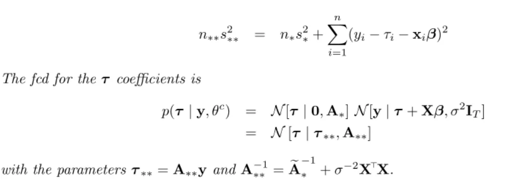
3. The fcd for the τ coefficients is

p(τ | y, θ

) = N [τ | 0, A

] N [y | τ + Xβ, σ

I

]

= N [τ | τ

, A

] (36)

with the parameters τ

= A

y and A

= A e

+ σ

X

X.

6. Regional extended HP filtering of GDP and employment

In this section we show how the spatial HP model can be applied to smooth the regional GDP and employment data across the 239 (contiguous) NUTS-2 regions in Europe for the year 2005. The data with the coordinates of the center points of the NUTS-2 regions are taken from EUROSTAT. The model we have specified is an extended HP model y = τ + Xβ + ε, where X contains the dummy variables for the 25 EU countries to catch the fixed effects plus an extra dummy variable Dagg for regions that are city agglomerations. The car driving times were obtained by own calculations based on pairwise queries by internet search machines and are used for the W matrix and to define the smoothing metric.

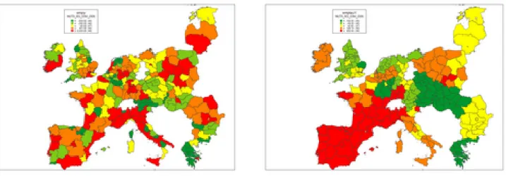
Figure 1: Spatial HP smooth of GDP 05, NUTS-2, 2005 Spatial HP smooth of Employment, NUTS-2, 2005

To define a smooth surface for a spatial cross-sectional data set we have to define a differencing matrix.

As it was shown in the above section, this can be easily done if we have a distance matrix between the

12

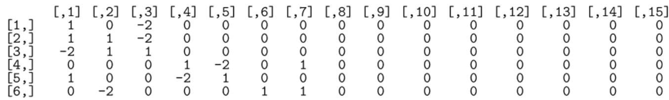
centers of the NUTS-2 regions. Thus we identify for each region a nearest neighbor (by distance) and a second nearest neighbor (also by distance). This produces the following K matrix, where - for demonstration - we display the first 6 rows.

[,1] [,2] [,3] [,4] [,5] [,6] [,7] [,8] [,9] [,10] [,11] [,12] [,13] [,14] [,15]

[1,] 1 0 -2 0 0 0 0 0 0 0 0 0 0 0 0

[2,] 1 1 -2 0 0 0 0 0 0 0 0 0 0 0 0

[3,] -2 1 1 0 0 0 0 0 0 0 0 0 0 0 0

[4,] 0 0 0 1 -2 0 1 0 0 0 0 0 0 0 0

[5,] 1 0 0 -2 1 0 0 0 0 0 0 0 0 0 0

[6,] 0 -2 0 0 0 1 1 0 0 0 0 0 0 0 0

The effect of the spatial smoothing is seen in alphabetical order of the 24 countries

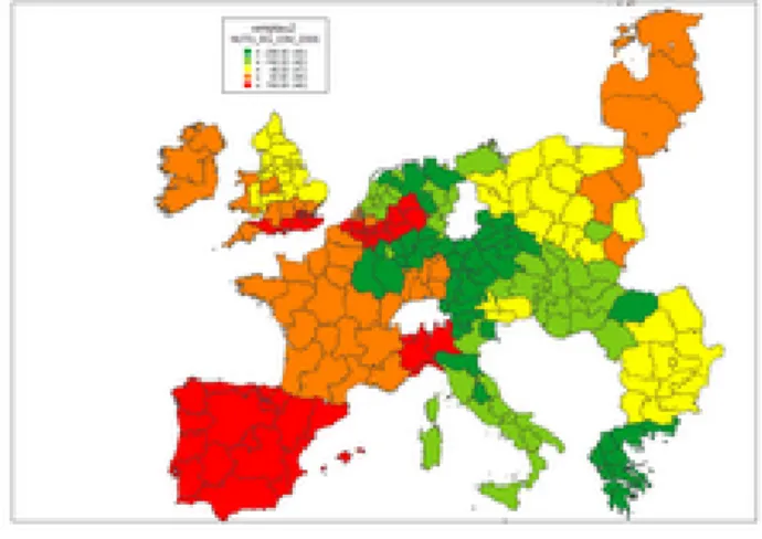
in Figure 1. The volatility of the smooth can be attributed to the heterogeneity between and within the countries. The median fixed effects coefficients of the extended spatial HP procedure were estimated with MCMC and are shown in Figure 2. These are the median effects of the 25 country dummy variables in X: The smallest one is Portugal and the largest one is Malta. The geographical maps for the smoothed GDP and GDPpc of NUTS-2 regions are given in the Figure 3 and in Figure 4, respectively, together with the observed raw values.

Figure 2: Median country effects in the extended spHP smooth of GDPpc, NUTS-2, 2005

lm(formula = log(y) ~ 0 + ZZ) Residuals:

Min 1Q Median 3Q Max

-3.00630 -0.40641 -0.02213 0.46751 2.22527 Coefficients:

Estimate Std. Error t value Pr(>|t|) Dagg 1.4260 0.6161 2.32 0.0216 * at 9.9837 0.2815 35.47 < 0.000 ***

be 9.8617 0.2607 37.83 < 0.000 ***

bg 8.0539 0.3448 23.36 < 0.000 ***

cy 9.5222 0.8445 11.28 < 0.000 ***

cz 9.3844 0.2986 31.43 < 0.000 ***

de 10.7655 0.1407 76.49 < 0.000 ***

ee 9.3245 0.8445 11.04 < 0.000 ***

es 10.1280 0.1937 52.28 < 0.000 ***

fi 9.6111 0.3777 25.45 < 0.000 ***

fr 10.8617 0.1800 60.33 < 0.000 ***

gr 9.3272 0.2815 33.14 < 0.000 ***

hu 9.2109 0.3192 28.86 < 0.000 ***

ie 11.0647 0.5971 18.53 < 0.000 ***

it 10.5937 0.1843 57.49 < 0.000 ***

3AT BE BG CY CZ DE EE E FI F GR HU IE I LT LU LV MT NL PL PT RO SK UK without DK SE SL

13

Figure 3: Spatial HP smooth of GDP NUTS-2, 2005 Map of 239 GDP NUTS-2 regions, 2005 (raw data)

Figure 4: Spatial HP smooth of GDPpc, NUTS-2, 2005 239 GDPpc NUTS-2 regions, 2005 (raw data)

lt 9.9366 0.8445 11.77 < 0.000 ***

lu 8.8840 1.0453 8.50 0.000 ***

lv 9.4736 0.8445 11.22 < 0.000 ***

mt 8.4671 0.8445 10.03 < 0.000 ***

nl 10.3268 0.2438 42.36 < 0.000 ***

pl 9.4063 0.2111 44.55 < 0.000 ***

pt 9.9515 0.3777 26.35 < 0.000 ***

ro 9.1704 0.2986 30.72 < 0.000 ***

sk 9.1493 0.4222 21.67 < 0.000 ***

uk 10.5717 0.1482 71.34 < 0.000 ***

Signif. codes: 0 *** 0.001 ** 0.01 * 0.05 ’.’ 0.1 ’’ 1 Residual standard error: 0.8445 on 214 degrees of freedom Multiple R-squared: 0.9939, Adjusted R-squared: 0.9931 F-statistic: 1386 on 25 and 214 df, p-value: < 2.2e-16 Ordered effects:

Dagg bg mt lu sk ro hu ee

1.426 8.054 8.467 8.884 9.149 9.170 9.211 9.325

gr cz pl lv cy fi be lt

9.327 9.384 9.406 9.474 9.522 9.611 9.862 9.937

pt at es nl uk it de fr ie

9.952 9.984 10.128 10.327 10.571 10.594 10.766 10.862 11.065

14

Figure 5: Spatial extended HP smooth of GDP Nuts-2, 2005 Spatial extended HP smooth of log GDP Nuts-2, 2005

6.1. Employment

Figure 6: Employment: NUTS-2, 2005 (raw data) MCMC Spatial HP smooth of Employment NUTS-2, 2005

Figure 6 shows the raw data together with the smooth of the employment data in 2005: the first things to note are the high employment effects in central Poland and Romania. The smooth in Figure 6 shows the smooth (posterior mean) of the spatial HP model while Figure 7 shows the smooth (posterior mean) of the spatial extended HP model. The X matrix of the extended model (eHP) just contains the fixed effect dummy variables for the countries plus an extra dummy for the new central and eastern European states (CEE). The border of the regions in the East and West of the smooth can be seen in both figures, which stretch until France. The somewhat unexpected map is due to the fact that German regions have less employment than the regions in Poland and Romania. Therefore we see higher smoothed values at the periphery and lower values in the center (Germany, the Czech Republic and Austria.) Also, by taking into account the large variation of levels across EU countries we see that these ”low smooth” values are still present in those 3 central European states.

15

Figure 7: MCMC of the spatial extended HP model, smooth of Employment NUTS-2, 2005

7. Model selection and Bayes testing

This section shows how to compute the Bayes factor for the HP smoother and to select the order of smoothness prior by marginal likelihoods. The assumption to do this requires a normal prior distribution with full rank. The first order differencing matrix is denoted as K

and the higher order differencing matrices are matrix powers: K

= K

and therefore the prior covariance matrix of the i-th smoothness model is A

= (λK

K

)

= (K

K)

/λ. For the conjugate normal-gamma regression model the marginal likelihood can be computed in closed form as the next theorem shows.

Theorem 5 (The marginal likelihood for the conjugate eHP model).

The marginal (data) likelihood (MDL) of the eHP regression model is given by a product of 3 factors (that are 3 ratios of prior to posterior parameters):

p(y | eHP ) = (π)

| A e

|

| A e

|

× Γ(

)

Γ(

) × (n

s

/2)

(n

s

/2)

, (37) where n

and s

are the posterior parameter given in (30) of Theorem 3.

Note that the marginal data likelihood for the HP model follows the ordinary MDL formula for the normal-gamma sampling model M DL

= p

(y)

p

(y) = (π)

× R

× R

× R

the ratio of determinants (R

), the ratio of d.f. (R

), and the ratio of residual variances (R

). Usually it is better to compute the lml = log(M DL) given by

lml

= − n

2 log(π) + log(R

) + log(R

) + log(R

). (38) The lml

times −2 is (with ESS

= n

s

/2 and ESS

= n

s

/2)

−2lml

= nlog(π) + log | A e

|

| A e

|

+ (n

−3)log(2) + 2log(Γ(n

− 1)) +n

log(ESS

)− n

log(ESS

). (39)

16

The ratio of determinants in the eHP model is computed by the inverses R

=| A e

| / | A e

|= | A

| n

|A

|| G

|

with A

= (λK

K

)

, A

= (I

+ λK

K

)

and G

= I − A

, where K

is the differencing matrix of order i.

Proof 5. The determinant of the prior is | A e

|=| A

| n

while for the determinant of the partitioned posterior we find

| A e

|=| A

|| G

| with G depending on the i-th differencing matrix: G

= n

I

+ X

P

X with P

as before. The ratio of determinants for differencing matrices of order i is

R

= | A e

|

| A e

|

= |λK

K

|

| I

+ λK

K

| n

| G

|

and the ESS ratio can be computed as

R

= (n

s

/2)

(n

s

/2)

= (n

s

/2)

((n

s

+ α

)/2)

. The ratio of d.f. (R

) is given for n

= 1 by Γ(1/2) = √

π and therefore we find R

= Γ(

)

Γ(

) = (n

− 2)!!

2

(40)

The log df-ratio is

log(R

) = log (n

− 2)!!

2

= (n

− 2)log(2) + log((n

− 2)!) − (n

− 1)

2 log(2) =

= (n

− 3)

2 log(2) + log(Γ(n

− 1)), (41)

because log(n

− 2)!! = (n

− 2)log(2) + log((n

− 2)!) and the double factorial is defined as (2k)!! = 2

· k!

.

4using|

E F

G H

|=|E||H−GE⁻¹F|

17

Theorem 6 (Bayes test between HP models of different smoothness order).

For the Bayes test between two eHP models of order i and j we need the Bayes factor (BF), which is defined as the ratio of the 2 marginal likelihoods of HP models and the BF is given by

BF = p(y | eHP

)

p(y | eHP

) = R

R

R

R

and the log BF is computed by

log(BF) = n

2 log n

s

+ α

+ p 2 log(n

) with α

the discrepancy factor of the smoothness model of order i:

α

= y

n

K

K

(n

K

K

+ Σ

)

Σ

y =

= y

(C

C/n

+ R

R)

y (42) with C

= K

and Σ

= (R

R)

. If n

= 1 then log(n

) = 0 and the second term vanishes.

Proof 6. The BF is given by the ratio of marginal likelihoods, with the ESS ratio of ratios (RoR) given by R

R

= ((n

s

+ α

)/2)

((n

s

+ α

)/2)

=

n

s

+ α

n

s

+ α

and the determinant ratio given by R

R

= | G

|

| G

|

| λK

K

|

| I

+ λK

K

| / | λK

K

|

|I

+ λK

K

| because the R

and the constant involving π cancels out.

The marginal likelihood for models M that are estimated by MCMC can be computed by the Newton- Raftery formula

ˆ

m(y | M)

= 1 n

n_rep

X

j=1 n

X

i=1

ln l(D

| M, θ

)

!

l(D

| M, θ)

(43) where D

= (y

, x

) is the i-th data observation and with the likelihood given by the HP model (23).

8. Summary

This paper has shown that the extended HP filter can be also used to smooth spatial regional data.

HP filtering is an over-parameterized regression problem from a Bayesian point that can be estimated in a conjugate normal-gamma model with a strong prior on the smoothness component. The large value of the smoothness parameter λ serves in the Bayesian model as a hypothetical sample size (of the prior information) for the smooth component τ , i.e. the parameter vector to be estimated. For the remaining coefficient we assume a small hypothetical sample size to express diffuse knowledge.

The Bayesian view of the extended HP procedure opens a new modeling technique for smoothing out- put variables in more complex econometric models. These are models that require more adjustments and simplifications before the smoothing procedure can be applied. The Bayesian interpretation of HP models shows how to obtain more flexibility via the prior information that is used for the estimation of the smooth and the non-smooth part in such a complex smoothing models. The non-conjugate estimation of the HP

18

model uses the MCMC approach and allows application of the HP smoothing approach to extended HP models for non-stationary data and to a spatial smoothing model as it is discussed in Polasek (2011a).

In the spatial context, the extended HP filter allows a spatial smoothing of data and this was demon- strated for the 239 NUTS-2 regions of the European Union for GDP and employment data. The smoothness in a spatial context is defined by the distance of neighboring regions. The spatial extended HP smoother can be computed easily using MCMC procedures of the linear regression model or the spatial autoregression (SAR) model. Possibly, this new family of extended HP procedures opens a new approach for smoothing output variables in more complex models that requires more adjustments and simplifications before the smoothing can be done. The Bayesian formulation allows to give more flexibility for the prior information that combines the smooth and the non-smooth part in such more complex HP-type smoothing models. Thus, our approach has demonstrated that econometric smoothing problems can be either embedded in simple univariate set-ups or in complex model-based applications.

9. Appendix: The Combination of Quadratic Forms

The standard result for combining quadratic forms in normal Bayes models is:

Theorem 7 (Combination of Quadratic Forms).

Let H and H

be two symmetric quadratic matrices. Then the sum of the two quadratic forms can be combined as

(β − b)

H(β − b) + (β − b

)

H

(β − b

)

= (β − b

)

H

(β − b

) + (b − b

)

H

(H

+ H)

H(b − b

) (44) with the parameters H

= H

+ H and b

= H

(H

b

+ Hb).

10. References

Cooley, T. F. and Prescott, E. C. (1995), Economic growth and business cycles. In Cooley, T. F., editor, Frontiers of Business Cycle Research, chapter 1. Princeton University Press, Princeton.

Da Fonseca C.M. (2005), On the eigenvalues of some tridiagonal matrices, J. Comput. Appl. Math.

200 (2007), no. 1, 283-286. Departamento de Matematica, Universidade de Coimbra, Preprint 05-16.

http://www.mat.uc.pt/preprints/ps/p0516.pdf

Hodrick, R, J. and E. C. Prescott (1980), Postwar U.S. Business Cycles: an Empirical Investigation, Discussion Paper no. 451, Carnegie Mellon University. Appeared (1997).

Hodrick, R.J. and E.P. Prescott (1997), Postwar Business Cycles: An Empirical Investigation, Journal of Money, Credit, and Banking, 29, 1-16.

King, Robert G. and Sergio T. Rebelo (1993), Low Frequency Filtering and Real Business Cycles, Journal of Economic Dynamics and Control vol. 17, no. 1-2, 207-231.

Kydland, Finn E. and Edward C. Prescott (1990), Business Cycles: Real Facts and a Monetary Myth, Federal Reserve Bank of Minneapolis Quarterly Review vol.14, 3-18.

Leser C.E.V. (1961), A Simple Method of Trend Construction, Journal of the Royal Statistical Society B, 23, 91-107.

Polasek W. (2011a), MCMC estimation of extended Hodrick-Prescott (HP) filtering models, IHS Vienna and RCEA discussion paper.

Polasek W. (2011b), The extended Hodrick-Prescott (eHP) filter as a conjugate regression model, IHS Vienna (Institute for Advanced Studies) discussion paper.

Polasek W. and R. Sellner (2011), Does Globalization affect Regional Growth? Evidence for EU27 NUTS-2 Regions, IHS Vienna and RCEA discussion paper.

Ravn, M. O. and H. Uhlig (2002), On Adjusting the HP-Filter for the Frequency of Observations, Review of Economics and Statistics, vol. 84(2), 371-76.

19

Author: Wolfgang Polasek

Title: The Extended Hodrick-Prescott (HP) Filter for Spatial Regression Smoothing

Reihe Ökonomie / Economics Series 275

Editor: Robert M. Kunst (Econometrics)

Associate Editors: Walter Fisher (Macroeconomics), Klaus Ritzberger (Microeconomics)

ISSN: 1605-7996

© 2011 by the Department of Economics and Finance, Institute for Advanced Studies (IHS),

Stumpergasse 56, A-1060 Vienna   +43 1 59991-0  Fax +43 1 59991-555  http://www.ihs.ac.at

ISSN: 1605-7996